The Consequences of Air Density Variations over Northeastern Scotland for Offshore Wind Energy Potential

 , and
, and
Abstract
:1. Introduction
2. Data and Methodology
2.1. Data
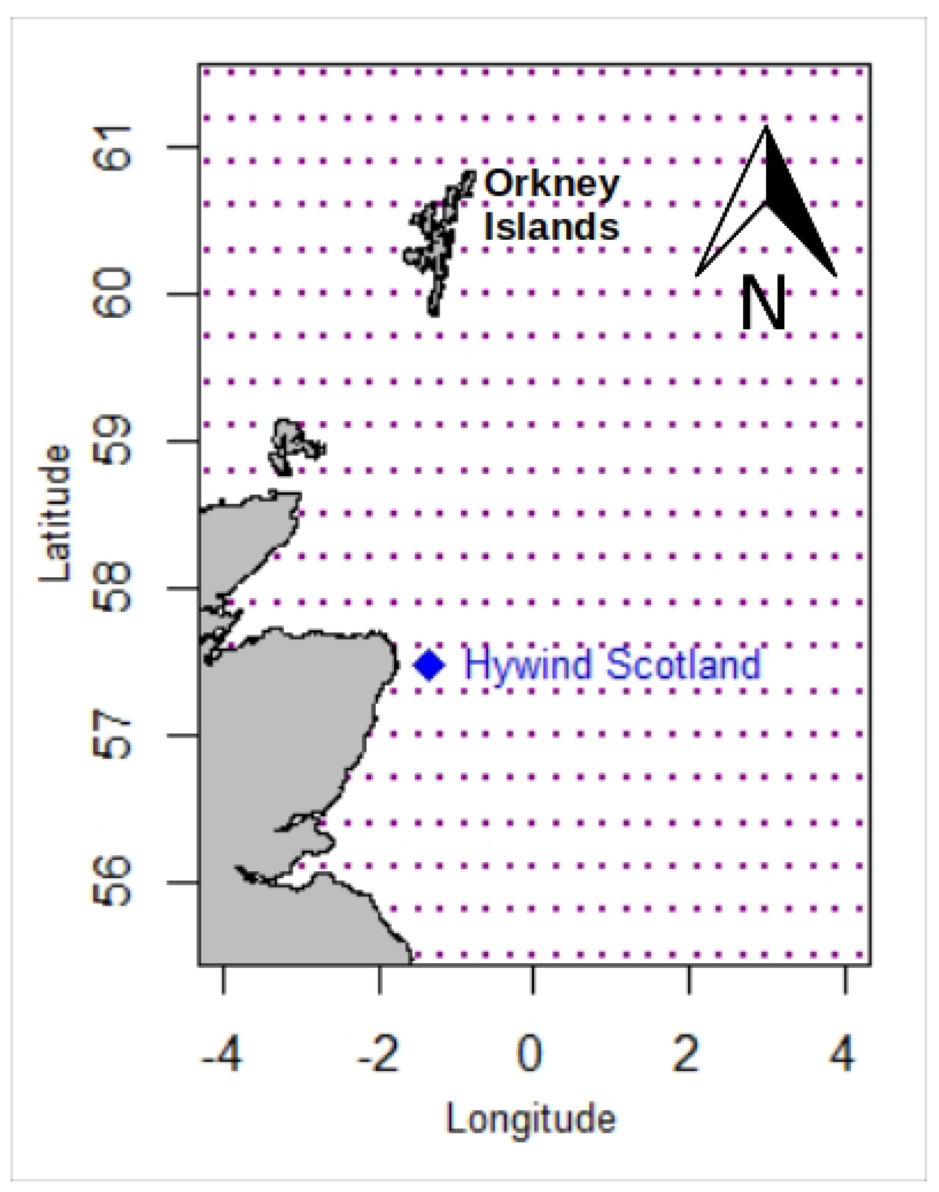
2.1.1. The ERA5 Reanalysis and the Study Area
2.1.2. SIEMENS 154/6 Floating Wind Turbine
2.2. Methodology
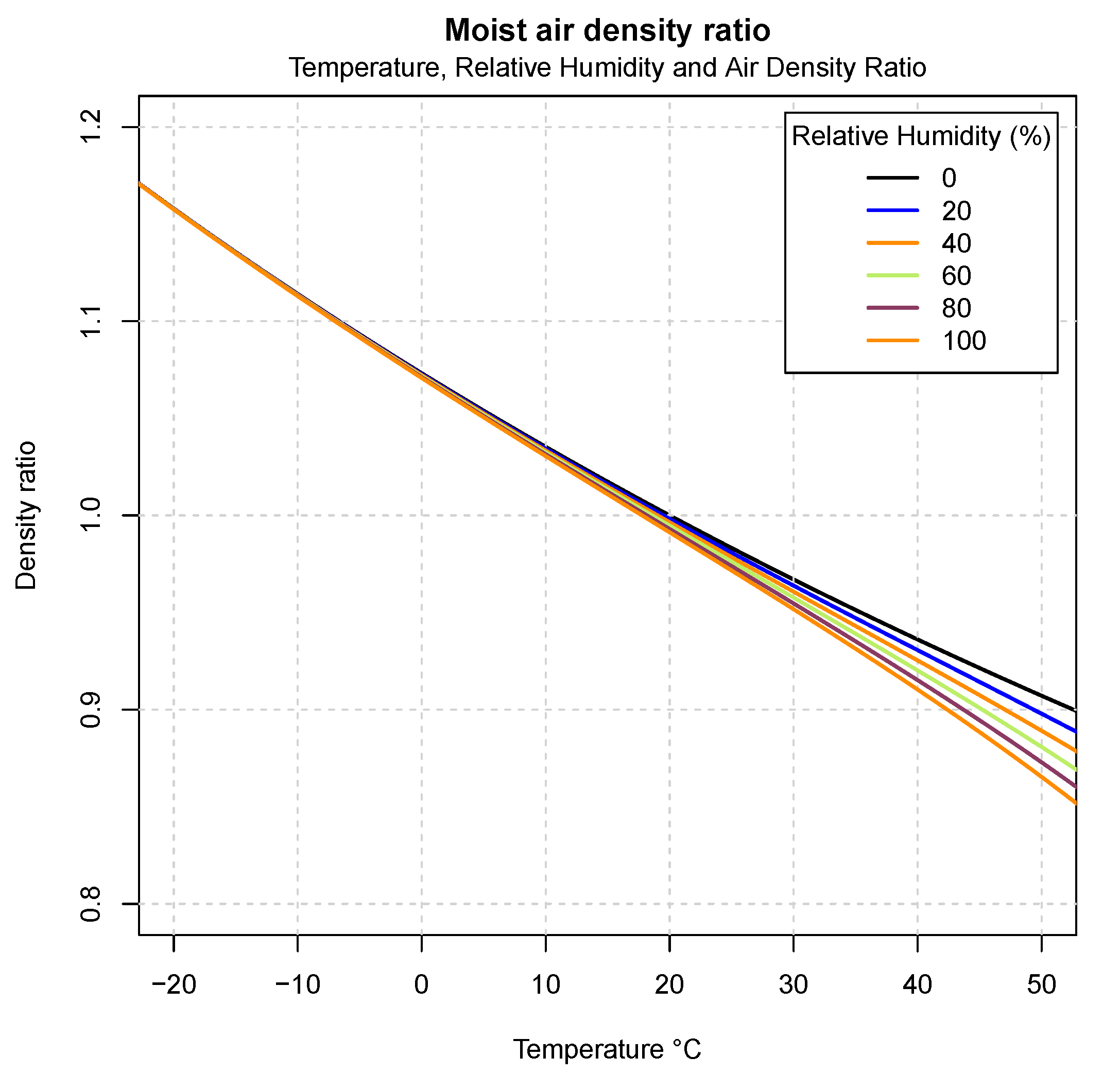
2.2.1. Air Density
2.2.2. Normalization of the Wind Speed According to Air Density
2.2.3. Capacity Factor and Energy Production
- Using the normalized wind speed from Equation (6) and therefore, incorporating the effect of air density changes ; and
- Using the observed wind speed associated with a constant value of 1.225 kg/m .
2.2.4. Analysis at Hywind-Scotland’s Nearest Gridpoint
- The hourly historical maximum and minimum air density values and their percentage variations with respect to the historical average value ( and ). Equation (9) shows the definition of given the historical maximum () and its mean (). The definition of would be equivalent:
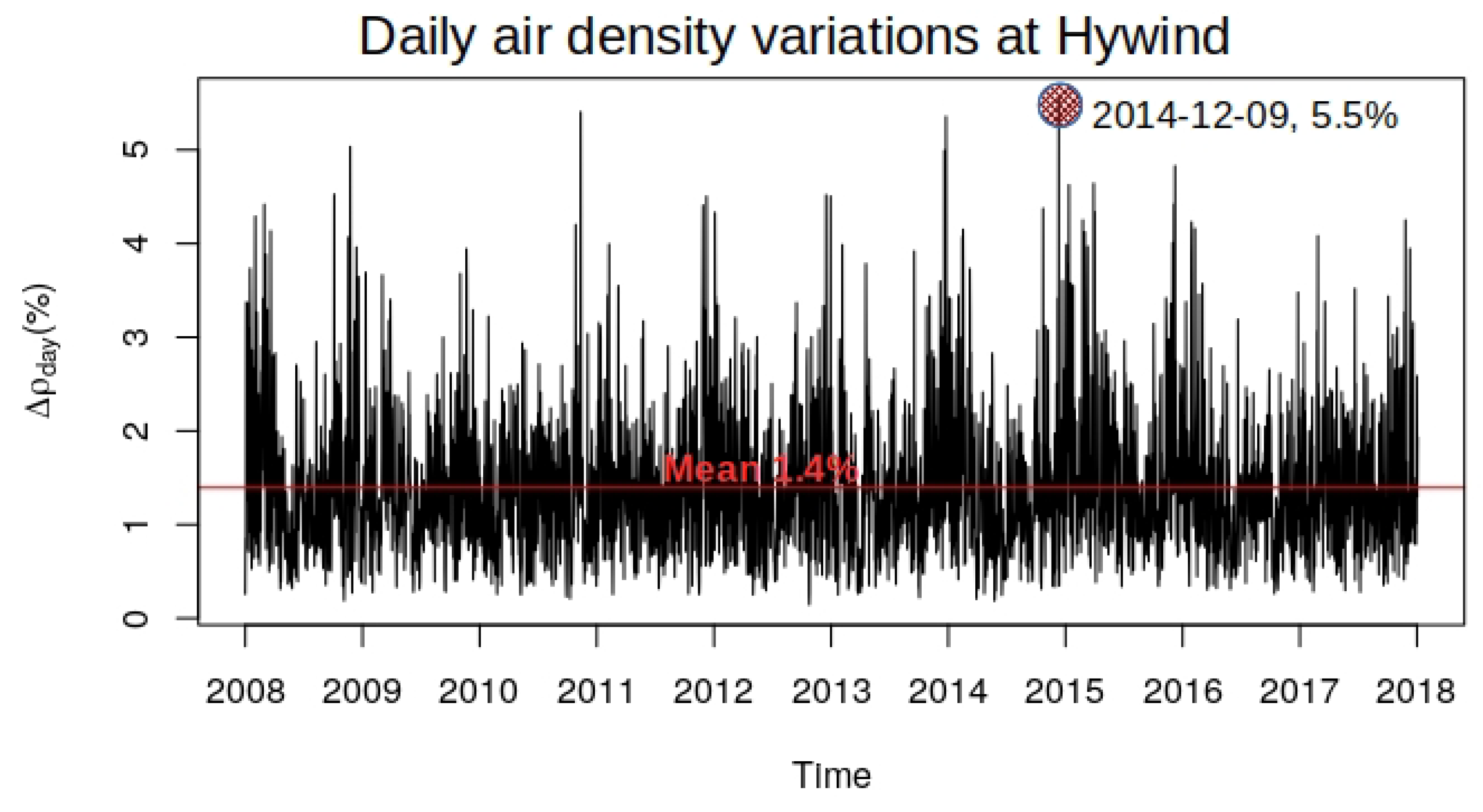
- Since hourly values are used, the intra-daily evolution of air density and effects such as the day–night cycle or land–sea breezes can be properly characterized. The characterization of cycles below 24 h is important, because 24 h is the leading studying horizon for wind energy farms [63]. A new parameter of deviation was defined, and the percentage deviation of the ratio between the minimum air density of the day d () and the maximum air density value of the day d () was used for that (Equation (10)):
2.2.5. Instantaneous Power Production Using FAST Simulations
3. Results
3.1. Map Representations
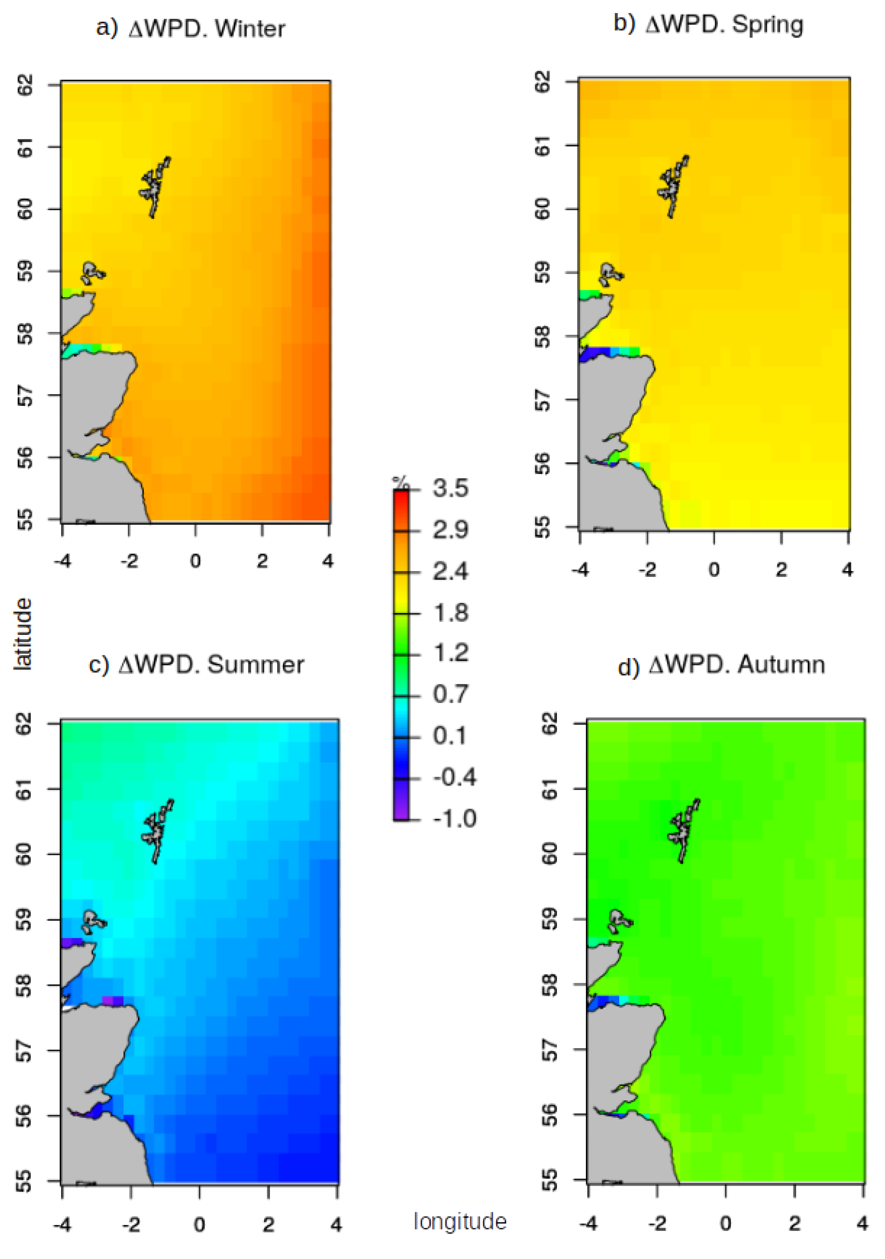
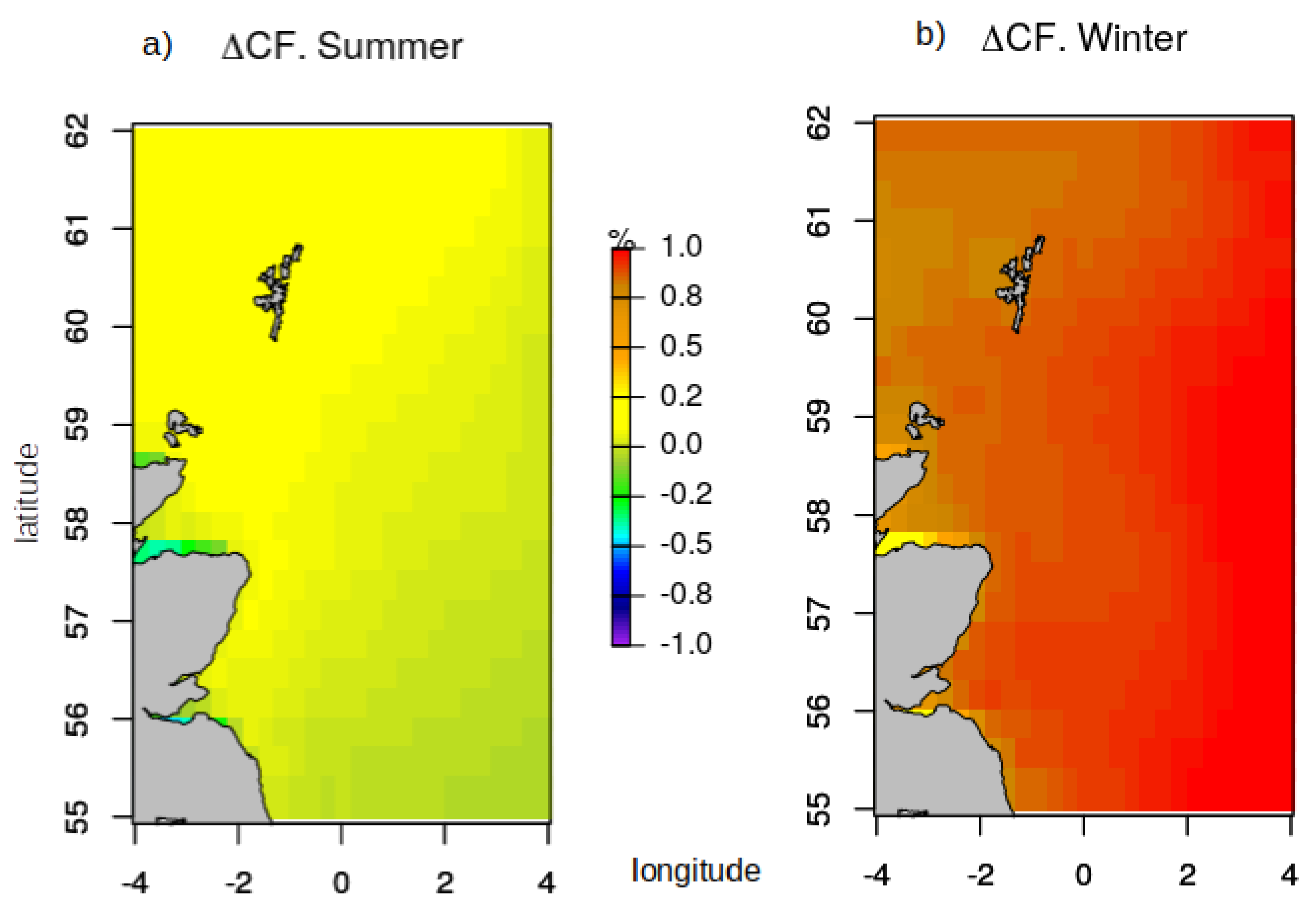
3.1.1. Seasonal Variations
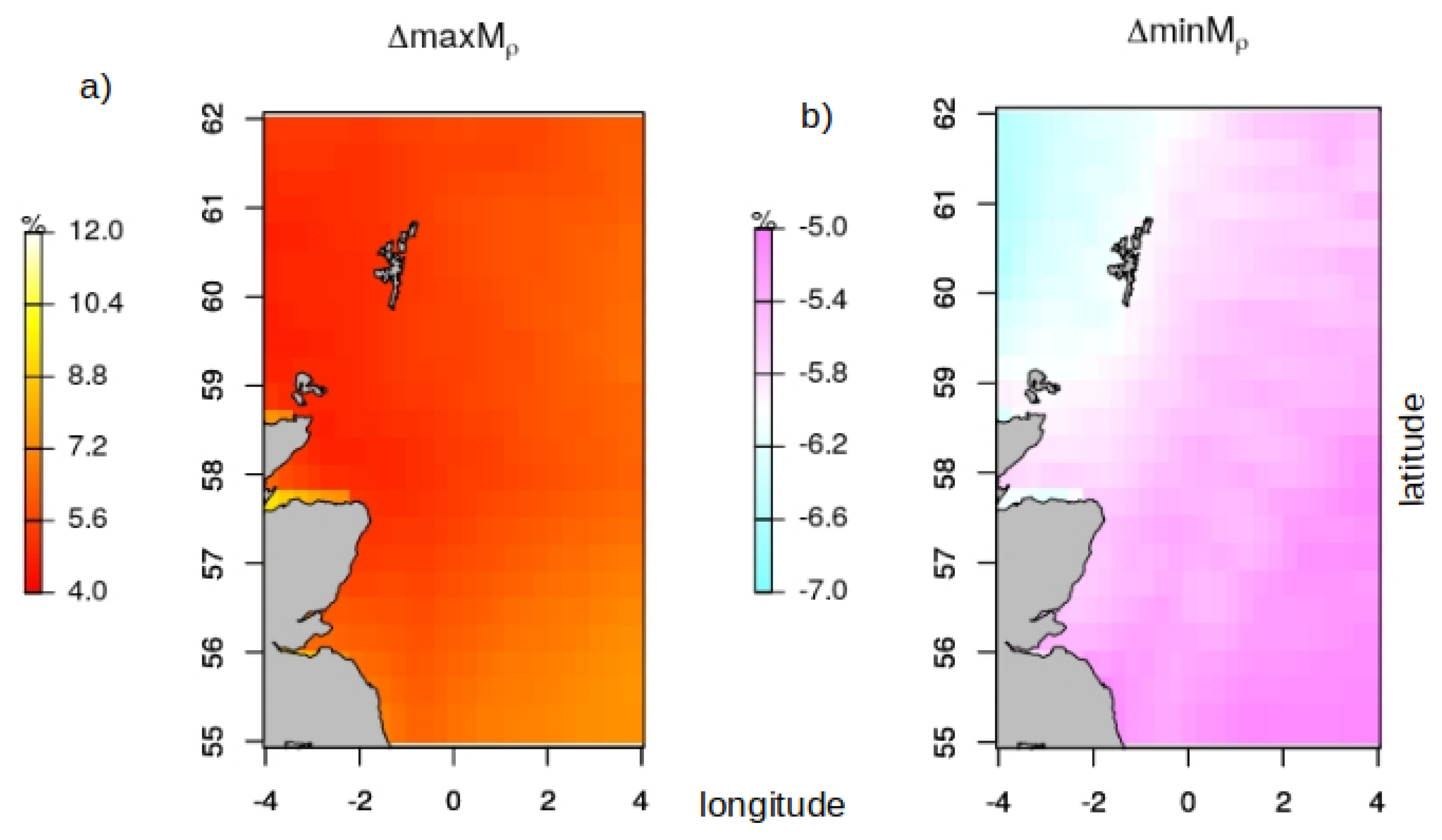
3.1.2. Maximum to Mean and Minimum to Mean Air Density Ratio Oscillations
3.2. Particular Case at Hywind Scotland
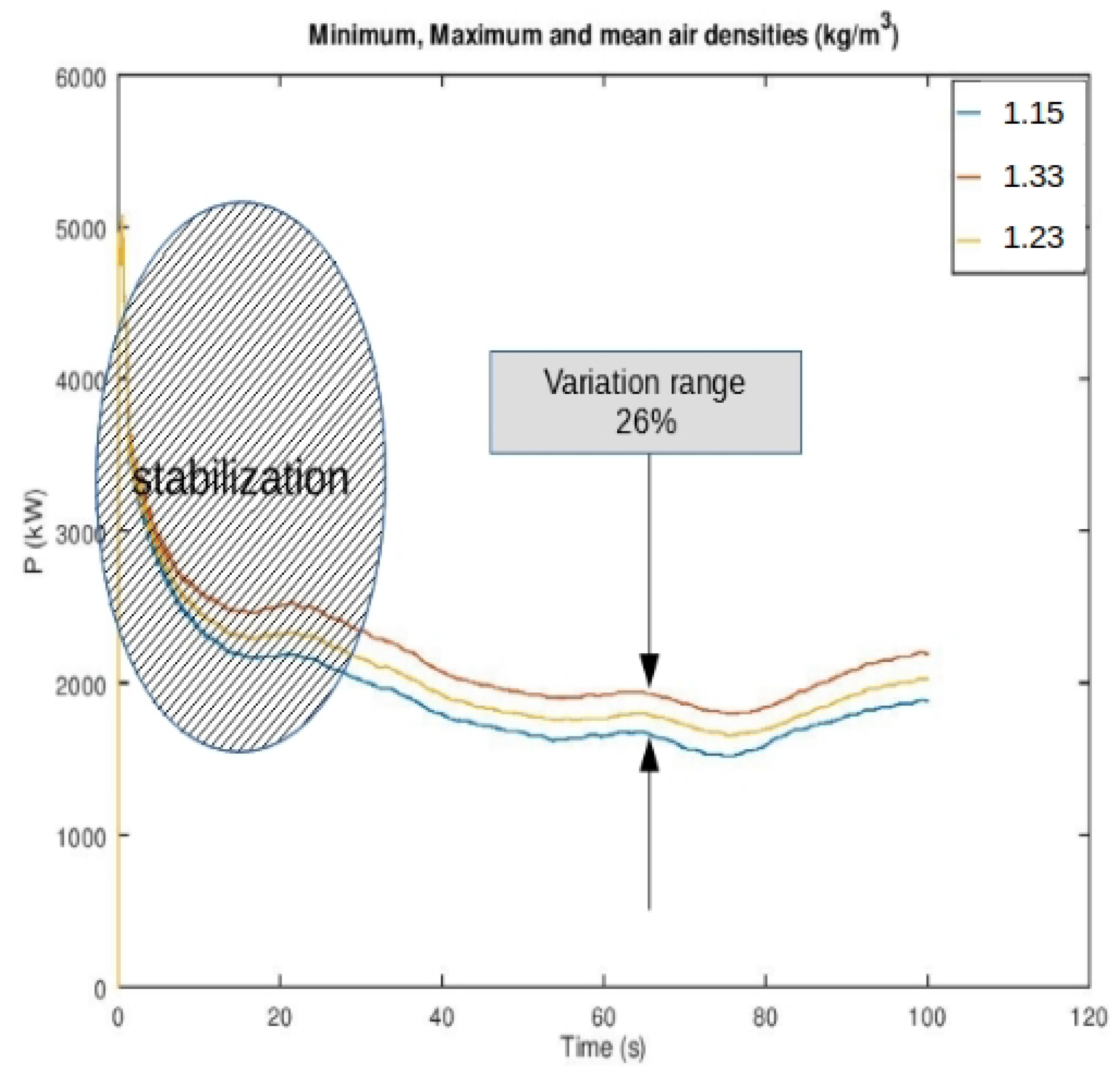
3.3. Simulation Using FAST
4. Discussion
- It has been shown that the observed variation of 2–3% for due to air density fluctuations in winter implies a subsequent of 1%. Thus, one turbine of 6 MW will produce 131 MWh more energy in winter than that estimated by the average air density at the site [11], which corresponds to 7860 US$ if a typical of 0.06 US$/kWh in wind energy is assumed [9]. This deviation of 1% is characteristic in Scottish waters, although variations from summer to winter can be higher. Besides, these economical deviations are approximately proportional to the nominal power of the considered turbine, and the most powerful turbines of the market (around 12 MW) would therefore, duplicate the profit in winter.
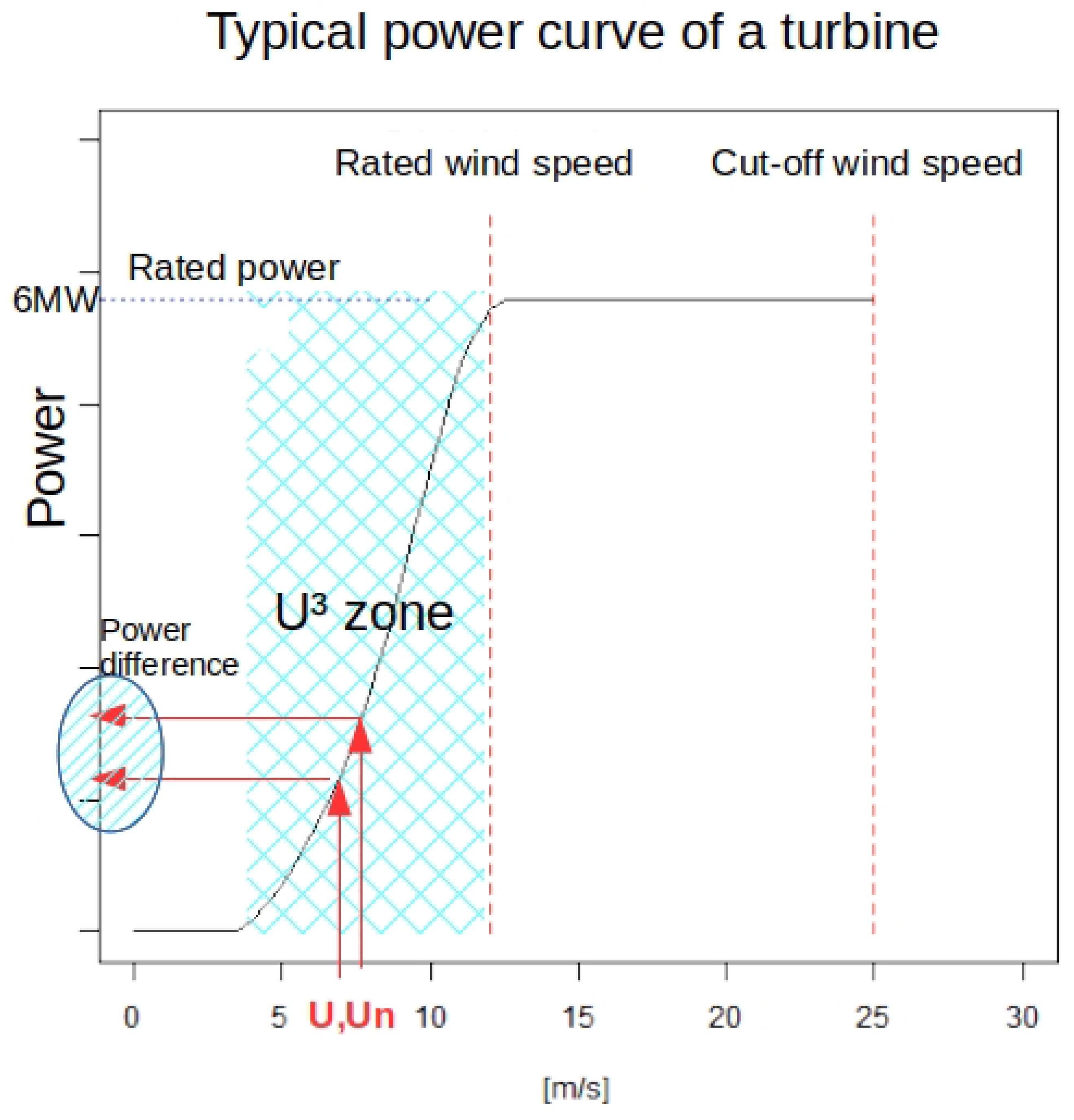
- By analyzing the impact that air density changes have in the instantaneous power generation described by the power curve of the turbine using hourly data, locations with maximum increments of 7% with respect to the average were found in the study area (see maps in Figure 5). The cubic root law of the normalization technique implies an increment of 2–3% for wind speed, which should be multiplied by three if the error in power is computed (Equation (11)). These estimated deviations that are near 10% in the zone of the power curve (see Figure 6) were corroborated using advanced simulations with the aeroelastic code FAST, as presented in Section 3.3.
- The maximum variations in air density within a given day at Hywind-Scotland show extreme cases that overcome the 5% with respect to the minimum of the day. These values are in the range within the order of magnitude of the previous historical maximum case, which imply similar power deviations. Instead of the seasonality of temperature, in the case of these daily fluctuations, sudden drops of pressure have been identified as the cause of strong air density changes.
- Events occurring within 24 h are very important for the wind energy industry, since the typical studying period is around this time range [63]. Thus, instead of only focusing on the provision of wind speed, the results of this work also indicate the necessity of air density short-term studies (pressure and temperature) for the wind industry.
- This aspect is also stressed for the Hywind-Scotland case, where in historical extreme cases, the instantaneous air density went from 1.17 to 1.35 kg/m, with almost proportional fluctuations in around the mean.
- Energy production losses in wind farms due to important mechanical or aerodynamic problems, such as pitch misalignment, present similar deviations [38]. Hence, the cause of energy production deviations can be confused with technical issues instead of related to questions about the wind resource and air density fluctuations.
5. Conclusions and Future Outlook
Author Contributions
Funding
Conflicts of Interest
Abbreviations
| ECMWF | European Centre for Medium-Range Weather Forecasts |
| WAsP | Wind Atlas Analysis and Application Program |
| WRF | Weather Research and Forecasting Model |
| Annual Energy Production (GWh) | |
| Capacity Factor (%) | |
| Capacity Factor computed with normalized wind speed (%) | |
| Cost of Energy ($/KWh) | |
| D | Wind turbine diameter (m) |
| Maximum to mean ratio of air density (%) | |
| Minimum to mean ratio of air density (%) | |
| P | Surface pressure (Pa) |
| Rated power of the wind turbine (kW) | |
| Seasonal Energy Production (GWh, MWh) | |
| T | Temperature (K) |
| U | Wind speed (m/s) |
| Normalized wind speed (m/s) | |
| Wind Power Density (W/m) | |
| Variation of CF (in percentage, %) | |
| Change in (in percent, %) | |
| Relative change in Wind Power Density (in percent, %) | |
| Change in air density (in percent, %) | |
| Change between maximum and minimum air density within a given day (in percent) | |
| Maximum air density in the day d (kg/m) | |
| Minimum air density in the day d (kg/m) | |
| Air density (kg/m) | |
| Standard air density (1.225 kg/m) |
References
- Grotjahn, R. Global Atmospheric Circulations: Observations and Theories; Oxford University Press: Oxford, UK, 1993; p. 450. [Google Scholar]
- James, I.N. Introduction to Circulating Atmospheres; Cambridge University Press: Cambridge, UK, 1994; p. 422. [Google Scholar]
- Vallis, G.K. Atmospheric and Oceanic Fluid Dynamics. Fundamentals and Large-Scale Circulation; Cambridge University Press: Cambridge, UK, 2006; p. 745. [Google Scholar]
- Warren, C.R.; Birnie, R.V. Re-powering Scotland: Wind farms and the ‘energy or environment?’ Debate. Scott. Geogr. J. 2009, 125, 97–126. [Google Scholar] [CrossRef]
- O’Keeffe, A.; Haggett, C. An investigation into the potential barriers facing the development of offshore wind energy in Scotland: Case study–Firth of Forth offshore wind farm. Renew. Sustain. Energy Rev. 2012, 16, 3711–3721. [Google Scholar] [CrossRef]
- Statoil Company. Technical Report. 2016. Available online: https://www.statoil.com/en/news/hywindscotland.html (accessed on 20 November 2016).
- Hersbach, H. The ERA5 Atmospheric Reanalysis. In AGU Fall Meeting Abstracts; American Geophysical Union: Washington, DC, USA, 2016. [Google Scholar]
- Olauson, J. ERA5: The new champion of wind power modelling? Renew. Energy 2018, 126, 322–331. [Google Scholar] [CrossRef] [Green Version]
- Manwell, J.F.; McGowan, J.G.; Rogers, A.L. Wind Energy Explained: Theory, Design and Application; John Wiley & Sons: Hoboken, NJ, USA, 2010. [Google Scholar]
- Floors, R.; Nielsen, M. Estimating Air Density Using Observations and Re-Analysis Outputs for Wind Energy Purposes. Energies 2019, 12, 2038. [Google Scholar] [CrossRef]
- Mortensen, N.G. 46200 Planning and Development of Wind Farms: Wind Resource Assessment Using the WAsP Software; DTU Wind Energy: Lyngby, Denmark, 2015. [Google Scholar]
- Monteiro, C.; Bessa, R.; Miranda, V.; Botterud, A.; Wang, J.; Conzelmann, G. Wind Power Forecasting: State-of-the-Art 2009; Technical report; Argonne National Laboratory (ANL): Lemont, IL, USA, 2009. [Google Scholar]
- Weisser, D. A wind energy analysis of Grenada: An estimation using the Weibull density function. Renew. Energy 2003, 28, 1803–1812. [Google Scholar] [CrossRef]
- Gökçek, M.; Bayülken, A.; Bekdemir, Ş. Investigation of wind characteristics and wind energy potential in Kirklareli, Turkey. Renew. Energy 2007, 32, 1739–1752. [Google Scholar] [CrossRef]
- Jiménez, P.A.; González-Rouco, J.F.; García-Bustamante, E.; Navarro, J.; Montávez, J.P.; de Arellano, J.V.G.; Dudhia, J.; Muñoz-Roldan, A. Surface wind regionalization over complex terrain: Evaluation and analysis of a high-resolution WRF simulation. J. Appl. Meteorol. Climatol. 2010, 49, 268–287. [Google Scholar] [CrossRef]
- Dvorak, M.J.; Archer, C.L.; Jacobson, M.Z. California offshore wind energy potential. Renew. Energy 2010, 35, 1244–1254. [Google Scholar] [CrossRef]
- Gross, M.S.; Magar, V. Offshore wind energy potential estimation using UPSCALE climate data. Energy Sci. Eng. 2015, 3, 342–359. [Google Scholar] [CrossRef]
- Akdağ, S.A.; Güler, Ö. Evaluation of wind energy investment interest and electricity generation cost analysis for Turkey. Appl. Energy 2010, 87, 2574–2580. [Google Scholar] [CrossRef]
- Fueyo, N.; Sanz, Y.; Rodrigues, M.; Montañés, C.; Dopazo, C. High resolution modelling of the on-shore technical wind energy potential in Spain. Wind Energy 2010, 13, 717–726. [Google Scholar] [CrossRef]
- Hasager, C.B.; Barthelmie, R.J.; Christiansen, M.B.; Nielsen, M.; Pryor, S. Quantifying offshore wind resources from satellite wind maps: study area the North Sea. Wind Energy 2006, 9, 63–74. [Google Scholar] [CrossRef]
- Doubrawa, P.; Barthelmie, R.J.; Pryor, S.C.; Hasager, C.B.; Badger, M.; Karagali, I. Satellite winds as a tool for offshore wind resource assessment: The Great Lakes Wind Atlas. Remote Sens. Environ. 2015, 168, 349–359. [Google Scholar] [CrossRef] [Green Version]
- Carvalho, D.; Rocha, A.; Santos, C.S.; Pereira, R. Wind resource modelling in complex terrain using different mesoscale–microscale coupling techniques. Appl. Energy 2013, 108, 493–504. [Google Scholar] [CrossRef]
- Carvalho, D.; Rocha, A.; Gómez-Gesteira, M.; Santos, C. A sensitivity study of the WRF model in wind simulation for an area of high wind energy. Environ. Model. Softw. 2012, 33, 23–34. [Google Scholar] [CrossRef] [Green Version]
- Carvalho, D.; Rocha, A.; Gómez-Gesteira, M.; Santos, C.S. Sensitivity of the WRF model wind simulation and wind energy production estimates to planetary boundary layer parameterizations for onshore and offshore areas in the Iberian Peninsula. Appl. Energy 2014, 135, 234–246. [Google Scholar] [CrossRef]
- Carvalho, D.; Rocha, A.; Gómez-Gesteira, M.; Santos, C.S. Comparison of reanalyzed, analyzed, satellite-retrieved and NWP modelled winds with buoy data along the Iberian Peninsula coast. Remote Sens. Environ. 2014, 152, 480–492. [Google Scholar] [CrossRef]
- Carvalho, D.; Rocha, A.; Gómez-Gesteira, M.; Santos, C.S. WRF wind simulation and wind energy production estimates forced by different reanalyses: Comparison with observed data for Portugal. Appl. Energy 2014, 117, 116–126. [Google Scholar] [CrossRef]
- Carvalho, D.; Rocha, A.; Gómez-Gesteira, M.; Santos, C.S. Offshore wind energy resource simulation forced by different reanalyses: Comparison with observed data in the Iberian Peninsula. Appl. Energy 2014, 134, 57–64. [Google Scholar] [CrossRef]
- Guerrero-Villar, F.; Dorado-Vicente, R.; Medina-Sánchez, G.; Torres-Jiménez, E. Alternative Calibration of Cup Anemometers: A Way to Reduce the Uncertainty of Wind Power Density Estimation. Sensors 2019, 19, 2029. [Google Scholar] [CrossRef]
- Farkas, Z. Considering air density in wind power production. arXiv 2011, arXiv:1103.2198. [Google Scholar]
- Collins, J.; Parkes, J.; Tindal, A. Short term studies for utility-scale wind farms. The power model challenge. Wind Eng. 2009, 33, 247–257. [Google Scholar] [CrossRef]
- Dahmouni, A.; Salah, M.B.; Askri, F.; Kerkeni, C.; Nasrallah, S.B. Assessment of wind energy potential and optimal electricity generation in Borj-Cedria, Tunisia. Renew. Sustain. Energy Rev. 2011, 15, 815–820. [Google Scholar] [CrossRef]
- Svenningsen, L. Power Curve Air Density Correction and Other Power Curve Options in WindPRO; Technical report; EMD International A/S: Aalborg, Denmark, 2010; Available online: www.emd.dk/files/windpro/WindPRO_Power_Curve_Options pdf (accessed on 15 May 2019).
- Ulazia, A.; Sáenz, J.; Ibarra-Berastegui, G. Sensitivity to the use of 3DVAR data assimilation in a mesoscale model for estimating offshore wind energy potential. A case study of the Iberian northern coastline. Appl. Energy 2016, 180, 617–627. [Google Scholar] [CrossRef]
- Ulazia, A.; Sáenz, J.; Ibarra-Berastegui, G.; González-Rojí, S.J.; Carreno-Madinabeitia, S. Using 3DVAR data assimilation to measure offshore wind energy potential at different turbine heights in the West Mediterranean. Appl. Energy 2017, 208, 1232–1245. [Google Scholar] [CrossRef] [Green Version]
- Yamaguchi, A.; Ishihara, T. Assessment of offshore wind energy potential using mesoscale model and geographic information system. Renew. Energy 2014, 69, 506–515. [Google Scholar] [CrossRef]
- Pourrajabian, A.; Mirzaei, M.; Ebrahimi, R.; Wood, D. Effect of air density on the performance of a small wind turbine blade: A case study in Iran. J. Wind Eng. Ind. Aerodyn. 2014, 126, 1–10. [Google Scholar] [CrossRef]
- Soraperra, G. Design of wind turbines for non-standard air density. Wind Eng. 2005, 29, 115–128. [Google Scholar] [CrossRef]
- Elosegui, U.; Egana, I.; Ulazia, A.; Ibarra-Berastegi, G. Pitch angle misalignment correction based on benchmarking and laser scanner measurement in wind farms. Energies 2018, 11, 3357. [Google Scholar] [CrossRef]
- Esteban, M.; Leary, D. Current developments and future prospects of offshore wind and ocean energy. Appl. Energy 2012, 90, 128–136. [Google Scholar] [CrossRef]
- Danook, S.H.; Jassim, K.J.; Hussein, A.M. The impact of humidity on performance of wind turbine. Case Stud. Therm. Eng. 2019, 14, 100456. [Google Scholar] [CrossRef]
- Jung, C.; Schindler, D. The role of air density in wind energy assessment—A case study from Germany. Energy 2019, 171, 385–392. [Google Scholar] [CrossRef]
- Dee, D.P.; Uppala, S.M.; Simmons, A.J.; Berrisford, P.; Poli, P.; Kobayashi, S.; Andrae, U.; Balmaseda, M.A.; Balsamo, G.; Bauer, P.; et al. The ERA-Interim reanalysis: Configuration and performance of the data assimilation system. Q. J. R. Meteorol. Soc. 2011, 137, 553–597. [Google Scholar] [CrossRef]
- Rabanal, A.; Ulazia, A.; Ibarra-Berastegi, G.; Sáenz, J.; Elosegui, U. MIDAS: A Benchmarking Multi-Criteria Method for the Identification of Defective Anemometers in Wind Farms. Energies 2019, 12, 28. [Google Scholar] [CrossRef]
- Aniskevich, S.; Bezrukovs, V.; Zandovskis, U.; Bezrukovs, D. Modelling the spatial distribution of wind energy resources in Latvia. Latvian J. Phys. Tech. Sci. 2017, 54, 10–20. [Google Scholar] [CrossRef]
- Sterl, S.; Liersch, S.; Koch, H.; van Lipzig, N.P.; Thiery, W. A new approach for assessing synergies of solar and wind power: Implications for West Africa. Environ. Res. Lett. 2018, 13, 094009. [Google Scholar] [CrossRef]
- Camargo, L.R.; Gruber, K.; Nitsch, F. Assessing variables of regional reanalysis datasets relevant for modelling small-scale renewable energy systems. Renew. Energy 2019, 133, 1468–1478. [Google Scholar] [CrossRef]
- Engelhorn, T.; Müsgens, F. How to estimate wind-turbine infeed with incomplete stock data: A general framework with an application to turbine-specific market values in Germany. Energy Econ. 2018, 72, 542–557. [Google Scholar] [CrossRef]
- Hörsch, J. PyPSA-Eur: An Open Optimization Model of the European Transmission System (Dataset). 2017. Available online: https://github.com/FRESNA/pypsa-eur (accessed on 15 May 2019).
- Allaerts, D.; Broucke, S.V.; van Lipzig, N.; Meyers, J. Annual impact of wind-farm gravity waves on the Belgian–Dutch offshore wind-farm cluster. J. Phys. 2018, 1037, 072006. [Google Scholar] [CrossRef]
- Sáenz, J.; González-Rojí, S.J.; Carreno-Madinabeitia, S.; Ibarra-Berastegi, G. aiRthermo: Atmospheric Thermodynamics and Visualization. R package version 1.2.1. 2018. Available online: https://cran.r-project.org/web/packages/aiRthermo/index.html (accessed on 15 May 2019).
- Sáenz, J.; González-Rojí, S.J.; Carreno-Madinabeitia, S.; Ibarra-Berastegi, G. Analysis of atmospheric thermodynamics using the R package aiRthermo. Comput. Geosci. 2019, 122, 113–119. [Google Scholar] [CrossRef]
- Ulazia, A.; Ibarra-Berastegi, G.; Sáenz, J.; Gonzalez-Rojí, S.J.; Carreno-Madinabeitia, S. Seasonal correction of offshore wind energy potential due to air density: Case of the Iberian Peninsula. Sustainability 2019, 11, 3648. [Google Scholar] [CrossRef]
- ECMWF. Part IV: Physical Processes. In IFS Documentation CY41R2; Number 4 in IFS Documentation; ECMWF: Reading, UK, 2016. [Google Scholar]
- United States Committee on Extension to the Standard Atmosphere. National Oceanic and Atmospheric Administration, Washington, DC (NOAA-S/T 76-15672): Supt. of Docs., US Gov Print Office (Stock No. 003-017-00323-0); United States Committee on Extension to the Standard Atmosphere: Washington, DC, USA, 1976. [Google Scholar]
- International Electrical Commission. Wind Turbines-Part 12-1: Power Performance Measurements of Electricity Producing Wind Turbines; IEC 61400-12-1; IEC: Geneva, Switzerland, 2005. [Google Scholar]
- Masters, G.M. Renewable and Efficient Electric Power Systems; John Wiley & Sons: Hoboken, NJ, USA, 2013. [Google Scholar]
- Casati, B.; Wilson, L.; Stephenson, D.; Nurmi, P.; Ghelli, A.; Pocernich, M.; Damrath, U.; Ebert, E.; Brown, B.; Mason, S. Forecast verification: Current status and future directions. Meteorol. Appl. 2008, 15, 3–18. [Google Scholar] [CrossRef]
- Moseley, S. From Observations to Forecasts–Part 12: Getting the most out of model data. Weather 2011, 66, 272–276. [Google Scholar] [CrossRef]
- Accadia, C.; Mariani, S.; Casaioli, M.; Lavagnini, A.; Speranza, A. Sensitivity of precipitation study skill scores to bilinear interpolation and a simple nearest-neighbor average method on high-resolution verification grids. Weather Forecast. 2003, 18, 918–932. [Google Scholar] [CrossRef]
- Borge, R.; Alexandrov, V.; Del Vas, J.J.; Lumbreras, J.; Rodriguez, E. A comprehensive sensitivity analysis of the WRF model for air quality applications over the Iberian Peninsula. Atmos. Environ. 2008, 42, 8560–8574. [Google Scholar] [CrossRef]
- Jiménez, P.A.; Dudhia, J. Improving the representation of resolved and unresolved topographic effects on surface wind in the WRF model. J. Appl. Meteorol. Climatol. 2012, 51, 300–316. [Google Scholar] [CrossRef]
- Soares, P.M.; Cardoso, R.M.; Miranda, P.M.; de Medeiros, J.; Belo-Pereira, M.; Espirito-Santo, F. WRF high resolution dynamical downscaling of ERA-Interim for Portugal. Clim. Dyn. 2012, 39, 2497–2522. [Google Scholar] [CrossRef]
- Lei, M.; Shiyan, L.; Chuanwen, J.; Hongling, L.; Yan, Z. A review on the studying of wind speed and generated power. Renew. Sustain. Energy Rev. 2009, 13, 915–920. [Google Scholar] [CrossRef]
- NWTC Information Portal (FAST). 2019. Available online: https://nwtc.nrel.gov/FAST (accessed on 10 March 2019).
- Kecskemety, K.M.; McNamara, J.J. Influence of wake dynamics on the performance and aeroelasticity of wind turbines. Renew. Energy 2016, 88, 333–345. [Google Scholar] [CrossRef]
- Guntur, S.; Jonkman, J.; Sievers, R.; Sprague, M.A.; Schreck, S.; Wang, Q. A validation and code-to-code verification of FAST for a megawatt-scale wind turbine with aeroelastically tailored blades. Wind Energy Sci. Discuss. 2017, 2, 1389738. [Google Scholar] [CrossRef]
- Guntur, S.; Jonkman, J.; Schreck, S.; Jonkman, B.; Wang, Q.; Sprague, M.; Hind, M.; Sievers, R. FAST v8 Verification and Validation for a Megawatt-Scale Wind Turbine with Aeroelastically Tailored Blades; Technical report; National Renewable Energy Lab. (NREL): Golden, CO, USA, 2016. [Google Scholar]
- Cyranoski, D. Renewable energy: Beijing’s windy bet. Nat. News 2009, 457, 372–374. [Google Scholar] [CrossRef] [PubMed]


| Stat. Ind. | (kg/m) | (%) |
|---|---|---|
| Min. | 1.15 | |
| 1rst qu. | 1.21 | |
| Mean | 1.23 | – |
| 3rd qu. | 1.25 | 1.8 |
| Max. | 1.33 | 8.9 |
© 2019 by the authors. Licensee MDPI, Basel, Switzerland. This article is an open access article distributed under the terms and conditions of the Creative Commons Attribution (CC BY) license (http://creativecommons.org/licenses/by/4.0/).
Share and Cite
Ulazia, A.; Nafarrate, A.; Ibarra-Berastegi, G.; Sáenz, J.; Carreno-Madinabeitia, S. The Consequences of Air Density Variations over Northeastern Scotland for Offshore Wind Energy Potential. Energies 2019, 12, 2635. https://doi.org/10.3390/en12132635
Ulazia A, Nafarrate A, Ibarra-Berastegi G, Sáenz J, Carreno-Madinabeitia S. The Consequences of Air Density Variations over Northeastern Scotland for Offshore Wind Energy Potential. Energies. 2019; 12(13):2635. https://doi.org/10.3390/en12132635
Chicago/Turabian StyleUlazia, Alain, Ander Nafarrate, Gabriel Ibarra-Berastegi, Jon Sáenz, and Sheila Carreno-Madinabeitia. 2019. "The Consequences of Air Density Variations over Northeastern Scotland for Offshore Wind Energy Potential" Energies 12, no. 13: 2635. https://doi.org/10.3390/en12132635