Analytical and Numerical Investigation of Fe₃O₄–Water Nanofluid Flow over a Moveable Plane in a Parallel Stream with High Suction

Abstract

In the current framework, a model is constituted to explore the impacts of high suction and partial slip on Fe₃O₄–water nanoliquid flow over a porous moveable surface in a parallel free stream. The mechanisms of heat transfer are also modeled in the existence of Newtonian heating effect. The obtaining PDEs are transformed into a non-linear ODE system employing appropriate boundary conditions to diverse physical parameters. The governing ODE system is solved using a singular perturbation technique that results in an analytical asymptotic solution as a function of the physical parameters. The obtained solution allows us to carry out an analytical parametric study to investigate the impact of the physical parameters on the nonlinear attitude of the system. The precision of the proposed method is verified by comparisons between the numerical and analytical results. The results confirm that the proposed technique yields a good approximation to the solution as well as the solution calculation has no CPU time-consuming or round off error. Numerical solutions are computed and clarified in graphs for the model embedded parameters. Moreover, profiles of the skin friction coefficient and the heat transfer rate are also portrayed and deliberated. The data manifests that both solid volume fraction and slip impact significantly alter the flow profiles. Moreover, an upward trend in temperature is anticipated for enhancing Newtonian heating strength. Additionally, it was found that both the nanofluid velocity and temperature distributions are decelerated when the solid volume fraction and suction parameters increase. Furthermore, a rise in slip parameter causes an increment in velocity profiles, and a rise in Biot number causes an increment in the temperature profiles.

1. Introduction

Recently, the investigation of solutions of nonlinear ordinary/partial differential equations is quite popular area of study. Such equations manifest in several physical, engineering and industrial applications. Most of nonlinear differential equations have no exact solution and then the numerical techniques have predominately been applied to handle such equations. The significance of gaining the analytical approximate solutions of nonlinear differential equations in mathematics and physics is yet still defying that requires novel techniques. Various researchers fundamentally had paid attention to investigate solutions of nonlinear differential equations by applying semi-analytical numerical methods such as Homotopy perturbation method [1], differential transform method [2], Homotopy analysis method [3], etc. The convergence of the series solutions obtained using these semi-analytical numerical methods are mainly dependent upon the initial guess and the smoothness of the solution. However for discontinuous or singularly perturbed nonlinear problems there does not exist a general theory or an efficient approach to find a good enough initial guess. Recently a new treatment of nonlinear boundary layer problems is introduced in [4,5] using singular perturbation techniques. The advantage of this method over other semi-analytical numerical methods is that as the boundary layer thickness decreases and the problem becomes much stiffer the accuracy of the obtained asymptotic solution increases.

The investigation of heat transfer over moveable surfaces is of great interest to researchers due to its engineering and industrial applications, such as glass fiber, the manufacture and drawing of plastics and rubber sheets, the cooling of continuous stripes and an infinite metallic sheet, paper production, continuous casting, the polymer extrusion process, food processing, and heat-treated materials travelling on conveyer belts. Sakiadis [6] initiated work on the analysis of boundary layer flow on a moving surface, which was later extended by Crane [7] by considering a linearly stretching surface. A theoretical and experimental investigation was done on the flow past a moveable surface by Tsou et al. [8]. Magyari and Keller [9,10] studied heat and mass transfer in the boundary layers on an exponentially stretching continuous surface. El-Kabeir et al. [11] investigated the unsteady MHD combined convection over a moving vertical sheet. Bataller [12] considered the radiation effects in the blasius flow over the moving surface. Ishak [13] reported the flow and heat transfer over a moving plate in a parallel stream. EL-Kabeir et al. [14] investigated unsteady MHD three dimensional by natural convection from an inclined stretching surface saturated porous medium. Rashad et al. [15] analyzed the viscous dissipation and ohmic heating effects on MHD mixed convection along a vertical moving surface. EL-Kabeir et al. [16] explored Heat transfer in a micropolar fluid flow past a permeable continuous moving surface.

Nanofluids, with the insight of their thermal conductivity improvement, have been found to be advantageous in diverse engineering and industrial applications. Working fluids have large requirements in terms of enhancing or reducing energy release to apparatuses and of their impacts based on thermal conductivity, heat capacity, and other physical properties in novel thermal and manufacturing processes. A weak thermal conductivity is one of the most salient parameters that can restrict the heat transfer performance. Additionally, conventional heat transfer fluids such as ethylene glycol, water, and engine oil have limited heat transfer abilities due to their weak thermal conductivity and consequently cannot assemble with modernistic cooling demands. On the other side, the thermal conductivity of metals is extremely large in comparison to classical heat transfer fluids. Suspending the ultrafine solid metallic particles in technological fluids leads to an enhancement in thermal conductivity. This is one of the most modern and convenient processes for enhancing the heat transfer coefficient. Choi and Eastman [17] were likely the first to employ a mixture of nanoparticles and base fluids. Such fluids were designated as nanofluids. Buongiorno [18] presented a comprehensive study concerning the heat transport in nanofluids and found an extraordinary rise in the thermal conductivity of nanofluids. The pattern of nanofluid suggested by Buongiorno [18] was applied as an instrument to study many nanofluids problems. Chamkha et al. [19] examined the unsteady hydro-magnetic flow of a nanofluid past a stretching sheet. Rashad et al. [20] analyzed the natural convection boundary layer of a non-Newtonian fluid about a permeable vertical cone embedded in a porous medium saturated with a nanofluid. Chamkha et al. [21] discussed the natural convection from a vertical permeable cone in nanofluid saturated porous media for uniform heat and nanoparticles volume fraction fluxes. For getting empirical correlations for engineering simulations, many efforts have been made on experimentally measuring the physical properties of nanofluids as well [22,23,24,25,26]. Choi [27] has also reported another model that examined various conventional fluids to examine the thermal conductivity of fluids with nanoparticle properties, and another is a model proposed by Tiwari and Das [28]. EL-Kabeir and co-authors [29,30] reported a theoretical analysis of the flow and heat transfer in a nanofluid. Rashad [31,32] investigated the impact of thermal MHD slip flow of a nanofluid over a nonisothermal wedge and an inclined stretching surface, respectively. Rashidi and co-authors [33,34,35,36,37] presented a comprehensive review of last theoretical and experimental studies on thermal conductivity of nanofluids. Li et al. [38] studied the effects of the Lorentz force and the induced anisotropic thermal conductivity due to a magnetic field on the flow and the heat transfer of a ferrofluid. Salleh et al. [39] investigated the magnetohydrodynamics flow past a moving vertical thin needle in a nanofluid with stability analysis.

The motivation of this investigation is thus to carry out an analytical parametric study through constructed analytical asymptotic solutions for the nanofluid passing through a moveable plane with constant velocity, in the same trend to the free stream taking into account the partial slip velocity, Newtonian heating and high suction effects. The accuracy of the proposed method is verified by comparisons between the numerical and analytical results. The results confirm that the suggested technique produces a good approximation to the solution as well as the solution calculation has no CPU time-consuming or round off error. Moreover, a numerical study is present and the results shown in figures confirm a high validation of the present parametric study.

The novelty of the present problem is the analysis of nanofluid flow over a moveable plane. This type of work has not been reported previously in the open literature. Another important aspect of this problem is the application of singular perturbation techniques for high suction condition for which the numerical solution is difficult.

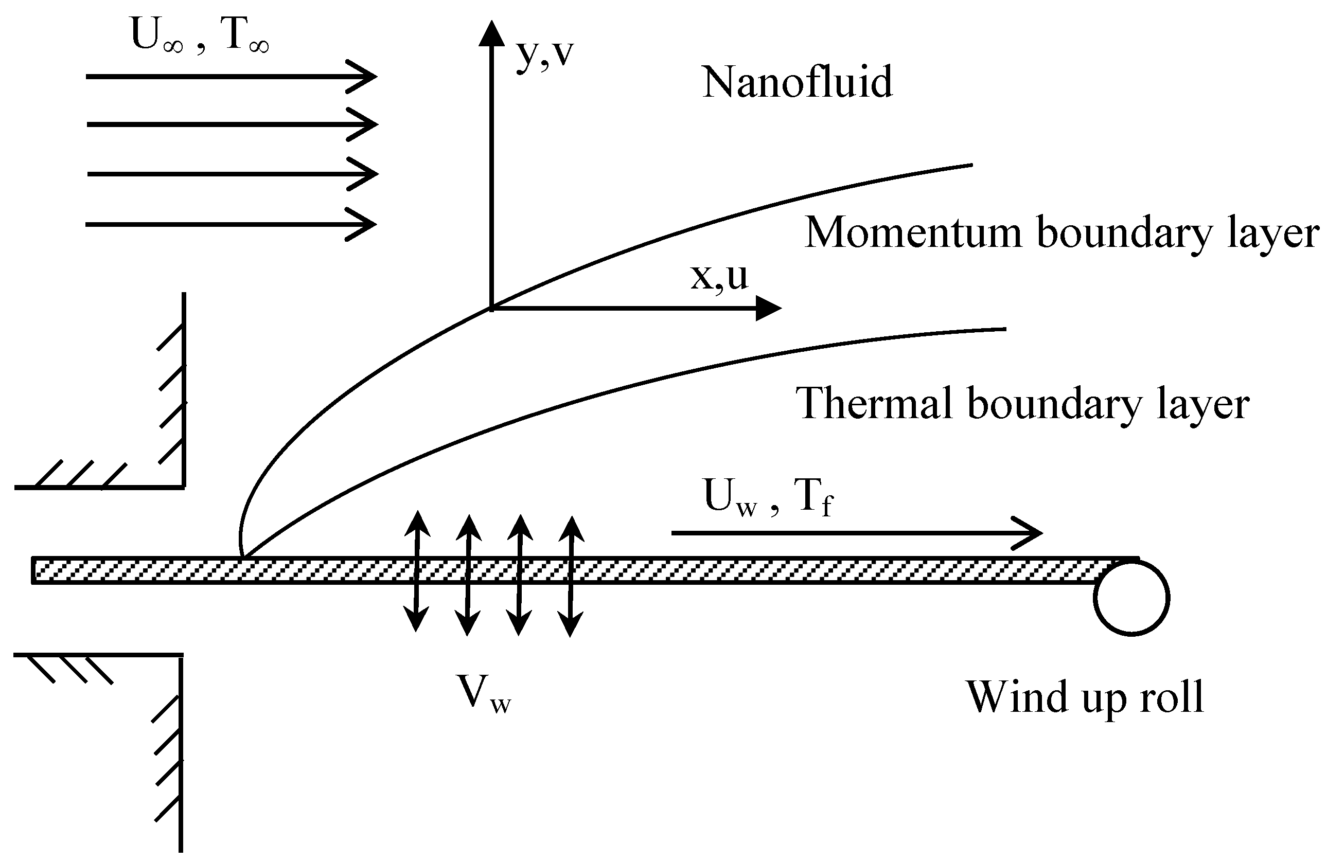
2. Modeling

Consider a steady 2D laminar flow of an iron oxide nanoparticle (Fe₃O₄)–water nanofluid passing through a moveable plane in parallel to a free stream of constant velocity U_w in parallel with a constant free stream velocity U_∞ with high fluid suction imposed on the surface. The flow pattern and physical coordinate system is demonstrated in Figure 1. In this coordinate frame, the x-axis extends in parallel to the surface, while the y-axis extends upwards, normal to the surface. The temperature at the plane surface is deemed to have a constant value T_f, which extends a heat transfer coefficient h_f while the ambient temperature has a constant value T_∞. The thermophysical properties of the nanofluid are given in

Table 1. Physical properties of base fluid and iron oxide nanoparticles [24,25].

Property	Pure Water	(Fe3O4)
ρ (kg m−3)	997.1	5200
Cp (Jkg−1 K−1)	4179	670
k (W m−1 K−1)	0.613	6

. In addition, both the base fluid (i.e., water) and the nanoparticles are in thermal equilibrium, and no slip occurs between them. With the above assumptions, the simplifying governing equations of the problem are

$$\frac{\partial u}{\partial x}+\frac{\partial v}{\partial y}=0$$

(1)

$$u\frac{\partial u}{\partial x}+v\frac{\partial u}{\partial y}=\frac{{\mu }_{nf}}{{\rho }_{nf}}\frac{{\partial }^{2}u}{\partial y^2}$$

(2)

$$u\frac{\partial T}{\partial x}+v\frac{\partial T}{\partial y}={\alpha }_{nf}\frac{{\partial }^{2}T}{\partial y^2}.$$

(3)

The associated boundary conditions of this problem can be written as

$$u=U_w+N{\mu }_{nf}\frac{\partial u}{\partial y},v=V_w,-k_{nf}\frac{\partial T}{\partial y}=h_f(T_f-T), \mathrm{at} y=0$$

(4a)

$$u=U_{\infty },T=T_{\infty }, \mathrm{at} y\to \infty .$$

(4b)

Here all parameters have been defined in the notation section. Additionally, ρ_nf, μ_nf, α_nf, (ρC_p), and (ρβ)_nf are defined as (see Tiwari and Das [28])

$${\rho }_{nf}=(1-\varphi ){\rho }_f+\varphi {\rho }_s, {\mu }_{nf}=\frac{{\mu }_f}{{(1-\varphi )}^{2.5}}, {\alpha }_{nf}=\frac{k_{nf}}{{\left(\rho C_p\right)}_{nf}}$$

(5)

$${\left(\rho C_p\right)}_{nf}=(1-\varphi ){\left(\rho C_p\right)}_f+\varphi {\left(\rho C_p\right)}_s$$

(6)

$$\frac{k_{nf}}{k_f}=\frac{\left(k_s+2k_f\right)-2\varphi \left(k_f-k_s\right)}{\left(k_s+2k_f\right)+\varphi \left(k_f-k_s\right)}.$$

(7)

We introduce the following non-dimensional variables:

$$\eta ={\left(\frac{U_w+U_{\infty }}{2{\upsilon }_{f}x}\right)}^{1/2}y, \psi ={\left(2{\upsilon }_{f}x\right)}^{1/2}{\left(U_w+U_{\infty }\right)}^{1/2}f(\eta ), \theta (\eta )=\frac{T-T_{\infty }}{T_f-T_{\infty }}$$

(8)

where ψ is the stream function defined in the usual way as $u=\partial \psi /\partial y$, $v=-\partial \psi /\partial x$. Substituting variables of Equation (8) into Equations (1)–(3) produces the following ordinary differential equations:

$$f^{‴}(\eta )+{(1-\varphi )}^{2.5}\left(1-\varphi +\varphi {\rho }_s/{\rho }_f\right)f(\eta )f^{″}(\eta )=0$$

(9)

$$\frac{1}{\mathrm{Pr}}\hspace{0.17em}\frac{k_{nf}/k_f}{\hspace{0.17em}1-\varphi +\varphi {(\rho C_P)}_s/{(\rho C_P)}_f}{\theta }^{″}(\eta )+f(\eta ){\theta }^{\prime }(\eta )=0,$$

(10)

and boundary conditions expressed in Equation (4) become

$$f(0)=f_w, f^{\prime }(0)=1-\gamma +\frac{\delta }{{(1-\phi )}^{2.5}}{f}^{″}(0), \underset{\ell \to {\infty }^{+}}{\lim }{f}^{\prime }(\ell )=\gamma$$

(11)

$$\frac{k_{nf}}{k_f}{\theta }^{\prime }(0)=-Bi(1-\theta (0)), \hspace{0.17em}\underset{\ell \to {\infty }^{+}}{\lim }\theta (\ell )=0$$

(12)

where primes denote the differentiation with respect to $\eta$, $f_w$ is the suction parameter, $\gamma$ is the velocity ratio parameter, $\delta$ is the velocity slip parameter, $Bi$ is the Biot number, and $\mathrm{Pr}$ is the Prantdl number, which are respectively defined as follows:

$$\begin{gathered} f_w=\frac{-2V_w{\left({\mathrm{Re}}_w+{\mathrm{Re}}_{\infty }\right)}^{1/2}}{\left(U_w+U_{\infty }\right)}, \gamma =\frac{U_{\infty }}{\left(U_w+U_{\infty }\right)}, \delta =N(x){\mu }_f{(\frac{U_W+U_{\infty }}{2{\nu }_{f}x})}^{1/2}, \\ Bi=\frac{h_f}{k_f}{(\frac{U_W+U_{\infty }}{2{\nu }_{f}x})}^{-1/2}, \mathrm{Pr}={\alpha }_f/{\upsilon }_f, {\mathrm{Re}}_w^{}=U_{w}x/{\upsilon }_f, {\mathrm{Re}}_{\infty }^{}=U_{\infty }x/{\upsilon }_f, \\ {\alpha }_f=k_f/{\left(\rho C_p\right)}_f, {\upsilon }_f={\mu }_f/{\rho }_f \end{gathered}$$

(13)

where Re_w and Re_∞ are the Reynolds numbers, ${\upsilon }_f$ is the kinematic coefficient of viscosity of base fluid, and α_f is the thermal diffusivity of base fluid.

Because the parameters δ and Bi depends on x, a true similarity is not accomplished. However, if the velocity slip coefficient N and the convection heat transfer coefficient h_f are proportional to $x^{-1/2}$, δ and Bi become independent of x and a true similarity is attained. It is manifested that the transpiration parameter f_w = 0 (V_w = 0) coincides with an impermeable surface, while f_w < 0 (V_w > 0) coincides to the status of fluid injection and f_w > 0 (V_w < 0) coincides to the status of the fluid suction or withdrawal (the current work). It is also manifested that velocity ratio parameters γ = 0 and γ = 1 coincides with a fixed plate in a moving fluid and with a moving plate in a quiescent fluid, respectively. The status 0 < γ < 1 is true when the plate and the fluid move in the same direction. If γ < 0, the free stream tends toward the positive x-direction, while the plate moves toward the negative x-direction. If γ > 1, the free stream is directed across the negative x-direction, while the plate moves across the positive x-direction. However, in this investigation, we inspect the status of γ ≤ 1, i.e., the direction of the free stream is specified (across the positive x-direction).

Of particular importance for this investigation are the local skin friction coefficient and the local Nusselt number. These physical quantities can be defined as

$$C_f=-\frac{{\mu }_{nf}{(\partial u/\partial y)}_{y=0}}{{\rho }_f{\left(U_w+U_{\infty }\right)}^2}, N{u}_x=\frac{k_{nf}{(\partial T/\partial y)}_{y=0}x}{k_f\left(T_w-T_{\infty }\right)}.$$

(14)

Applying the non-dimensional variables of Equation (8), we obtain

$$C_f{\left({\mathrm{Re}}_w+{\mathrm{Re}}_{\infty }\right)}^{1/2}=-\frac{1}{\sqrt{2}{(1-\varphi )}^{2.5}}{f}^{″}(0), N{u}_x{\left({\mathrm{Re}}_w+{\mathrm{Re}}_{\infty }\right)}^{-1/2}=-\frac{1}{\sqrt{2}}\frac{k_{nf}}{k_f}{\theta }^{\prime }(0).$$

(15)

3. Analytical Solutions via Singular Perturbation Technique

For larger suction parameter value $f_w$, the BVP (9)–(12) becomes much stiffer or singularly perturbed and the standard numerical methods fail to handle this situation unless we use special purpose methods or numerical routines for stiff differential equations with continuation techniques [40,41,42,43,44,45,46,47,48,49,50,51]. In general the numerical solution of a stiff or singularly perturbed BVP will be more difficult matter than the numerical solution of the corresponding IVPs. Hence, we prefer to approximate the BVPs (9)–(12) by suitable IVPs. For convenience, based on singular perturbation theory [40,41,50] and the formulation developed early by El-Zahar and EL-Kabeir [51], the BVPS (9)–(12) can approximated by IVPs with known closed form analytical asymptotic solutions.

3.1. An Analytical Solution of Energy Equation

Equation (10) with the boundary conditions of Equation (12) can be written as

$$\epsilon \hspace{0.17em}{\theta }_1^{″}(t)+f_1(t)\hspace{0.17em}{\theta }_1^{\prime }(t)=0, {\theta }_{{}_1}(0)=A\hspace{0.17em},\hspace{0.17em}\hspace{0.17em}\hspace{0.17em}\hspace{0.17em}\hspace{0.17em}{\theta }_{{}_1}(1)=0$$

(16)

where $\epsilon =\frac{\sigma }{\ell }$, $\sigma =\frac{1}{\mathrm{Pr}}\hspace{0.17em}\frac{k_{nf}/k_f}{\hspace{0.17em}1-\varphi +\varphi {(\rho C_P)}_s/{(\rho C_P)}_f}$, $0<\epsilon \ll 1$, $t=\frac{\eta }{\ell }$, ${\theta }_1(t)=\theta (\eta )$, $f_1(t)=f(\eta )$, and $f_1(t)\ge \hspace{0.17em}\hspace{0.17em}\hspace{0.17em}{f}_w\gg 0$ for every $t\in \hspace{0.17em}[\hspace{0.17em}0,\hspace{0.17em}1]$, and $A$ is a constant to be determined. Under these assumptions, the solution of Equation (16) has a boundary layer of width $O(\epsilon /f_w)$ at $t=0$ [4,5,40,41].

Setting $\epsilon =0$ in Equation (16) results in a reduced solution $\hspace{0.17em}{\theta }_0(t)=0$ that satisfies the reduced IVP:

$$f_1(t)\hspace{0.17em}\hspace{0.17em}{\theta }_0^{\prime }(t)=0\hspace{0.17em},\hspace{0.17em}\hspace{0.17em}\hspace{0.17em}\hspace{0.17em}\hspace{0.17em}\hspace{0.17em}\hspace{0.17em}\hspace{0.17em}\hspace{0.17em}{\theta }_0(1)=0,$$

(17)

and an approximate singularly perturbed IVP to (16) is thus obtained and given by [40,41,49,50].

$$\epsilon \hspace{0.17em}{\theta }_1^{\prime }(t)+f_1(t)\hspace{0.17em}\hspace{0.17em}{\theta }_1(t)=O(\epsilon /f_w),\hspace{0.17em}\hspace{0.17em}\hspace{0.17em}\hspace{0.17em}\hspace{0.17em}\hspace{0.17em}{\theta }_{{}_1}(1)=A\hspace{0.17em},$$

(18)

which has a zeroth order asymptotic solution $\overline{{\theta }_1}(t)$ given by [40,41,49,50]

$$\overline{{\theta }_1}(t)=A{e}^{-f_w\hspace{0.17em}t/\epsilon }.$$

(19)

Using Equations (19) and (12), the constant $A$ is determined and an asymptotic solution $\overline{\theta }(\eta )$ to the energy equation is obtained and given by

$$\overline{\theta }(\eta )=\frac{\sigma Bi\hspace{0.17em}{k}_f}{\hspace{0.17em}{f}_w\hspace{0.17em}{k}_{nf}+\sigma Bi\hspace{0.17em}{k}_f}{e}^{-f_w\hspace{0.17em}\eta /\sigma },$$

(20)

which results in

$${\overline{\theta }}^{\prime }(\eta )=-\frac{f_{w}Bi\hspace{0.17em}{k}_f}{\hspace{0.17em}{f}_w\hspace{0.17em}{k}_{nf}+\sigma Bi\hspace{0.17em}{k}_f}{e}^{-f_w\hspace{0.17em}\eta /\sigma }.$$

(21)

Theorem 1.

Let $\theta (\eta )$ and $\overline{\theta }(\eta )$ be respectively the solution of Equation (10) with its boundary conditions expressed by Equation (12) and the solution given by Equation (20), respectively. Then we have the following bounded error:

$$\left|\theta (\eta )\hspace{0.17em}-\hspace{0.17em}\overline{\theta }(\eta )\right|\hspace{0.17em}\hspace{0.17em}\le C\hspace{0.17em}\left(\frac{\varphi Bi\hspace{0.17em}}{\hspace{0.17em}{f}_w^2\hspace{0.17em}+f_{w}Bi\hspace{0.17em}}\hspace{0.17em}\right)$$

(22)

where $C$ is a positive constant independent of $\varphi$, $Bi$ and $f_w$.

Proof. 

For ${\theta }_1(t)$ and $\overline{{\theta }_1}(t)$, we have [40,41,45,49,50]

$$\begin{array}{l}\left|{\theta }_1(t)\hspace{0.17em}-\hspace{0.17em}\overline{{\theta }_1}(t)\right|\hspace{0.17em}\le C_1{\displaystyle \underset{t}{\overset{1}{\int }}\left|{\theta }_1(s)-{\theta }_0(s)\right|}\hspace{0.17em}ds\hspace{0.17em}\hspace{0.17em}\\ \hspace{0.17em}\hspace{0.17em}\hspace{0.17em}\hspace{0.17em}\hspace{0.17em}\hspace{0.17em}\hspace{0.17em}\hspace{0.17em}\hspace{0.17em}\hspace{0.17em}\hspace{0.17em}\hspace{0.17em}\hspace{0.17em}\hspace{0.17em}\hspace{0.17em}\hspace{0.17em}\hspace{0.17em}\hspace{0.17em}\hspace{0.17em}\hspace{0.17em}\hspace{0.17em}\le C\hspace{0.17em}\left|{\theta }_1(0)\frac{\epsilon \hspace{0.17em}}{f_w}\right|\end{array}$$

(23)

$$\le C\hspace{0.17em}\left|\frac{{\sigma }^{2}Bi\hspace{0.17em}}{\hspace{0.17em}{f}_w^2\hspace{0.17em}{k}_{nf}/k_f+\sigma Bi\hspace{0.17em}{f}_w}\right|$$

Since $k_s>k_f>0$, ${(\rho C_P)}_s>{(\rho C_P)}_f>0$, and $0\le \varphi <0.5$, $k_{nf}\hspace{0.17em},\hspace{0.17em}\hspace{0.17em}\sigma \hspace{0.17em}\propto \hspace{0.17em}\varphi$, and changing $t$ to $\eta$ in Equation (23) results in

$$\left|\theta (\eta )\hspace{0.17em}-\hspace{0.17em}\overline{\theta }(\eta )\right|\hspace{0.17em}\hspace{0.17em}\le C\hspace{0.17em}\left(\frac{\varphi Bi\hspace{0.17em}}{\hspace{0.17em}{f}_w^2\hspace{0.17em}+f_{w}Bi\hspace{0.17em}}\hspace{0.17em}\right).$$

☐

3.2. An Analytical Solution of the Blasuis Equation

Using the same procedure, we obtain an analytical solution to the Blasuis equation as follows.

Equation (9) with its boundary conditions expressed by Equation (11) can be written as

$$g^{″}(\eta )+h(\eta )g^{\prime }(\eta )=0, \hspace{0.17em}g(0)=\gamma +\frac{\delta }{{(1-\phi )}^{2.5}}{g}^{\prime }(0),\hspace{0.17em}\hspace{0.17em}\hspace{0.17em}\underset{\ell \to {\infty }^{+}}{\lim }\hspace{0.17em}\hspace{0.17em}g(\ell )=1-\gamma$$

(24)

where $g(\eta )=f^{\prime }(\eta )$, $h(\eta )=K_{\varphi }\hspace{0.17em}f(\eta )$ and $K_{\varphi }={(1-\varphi )}^{2.5}\left(1-\varphi (1-{\rho }_s/{\rho }_f)\right)$.

Changing variable $\eta$ to $x=\frac{\eta }{\ell }$, the BVP of Equation (24) becomes

$$\kappa g_1^{″}(x)+h_1(x)g_1^{\prime }(x)=0, \hspace{0.17em}{g}_1(0)=\gamma +\frac{\delta }{\ell {(1-\phi )}^{2.5}}{g}_1^{\prime }(0),\hspace{0.17em}\hspace{0.17em}\hspace{0.17em}\hspace{0.17em}{g}_1(1)=1-\gamma$$

(25)

where $\kappa =\frac{1}{\ell }$ $g_1(x)=g(\eta )$ and $h_1(x)=h(\eta )$.

The BVP of Equation (25) has a zeroth order asymptotic solution [40,41,49,50] given by

$${\overline{g}}_1(x)=(1-\gamma )+\frac{{\left(1-\varphi \right)}^{5/2}\left(2\mathsf{\gamma }-1\right){\mathrm{e}}^{-K_{\varphi }{f}_w\hspace{0.17em}x/\kappa }}{K_{\varphi }\hspace{0.17em}\hspace{0.17em}{f}_w\mathsf{\delta }+{\left(1-\varphi \right)}^{5/2}}.$$

(26)

Thus, we have the following approximation to $f^{\prime }(\eta )$

$${\overline{f}}^{\prime }(\eta )=(1-\gamma )+\frac{{\left(1-\varphi \right)}^{5/2}\left(2\mathsf{\gamma }-1\right){\mathrm{e}}^{-K_{\varphi }{f}_w\hspace{0.17em}\eta }}{K_{\varphi }\hspace{0.17em}\hspace{0.17em}{f}_w\mathsf{\delta }+{\left(1-\varphi \right)}^{5/2}}, \mathrm{with} \hspace{0.17em}\overline{f}(0)=f_w.$$

(27)

The solution of Equation (23) is approximated by

$$\overline{f}(\eta )=f_w+(1-\gamma )\eta +\frac{\left(2\mathsf{\gamma }-1\right){\left(1-\varphi \right)}^{5/2}}{K_{\varphi }\hspace{0.17em}\hspace{0.17em}{f}_w\left(k_{\varphi }\hspace{0.17em}\hspace{0.17em}{f}_w\mathsf{\delta }+{\left(1-\varphi \right)}^{5/2}\right)}(1-e^{-f_w\hspace{0.17em}{K}_{\varphi }\hspace{0.17em}\eta }),$$

(28)

which results in

$${\overline{f}}^{″}(\eta )=-\frac{{\left(1-\varphi \right)}^{5/2}\left(2\mathsf{\gamma }-1\right)K_{\varphi }\hspace{0.17em}\hspace{0.17em}{f}_w}{K_{\varphi }\hspace{0.17em}\hspace{0.17em}{f}_w\mathsf{\delta }+{\left(1-\varphi \right)}^{5/2}}{\mathrm{e}}^{-K_{\varphi }{f}_w\hspace{0.17em}\eta }.$$

(29)

Theorem 2.

Let $f^{\prime }(\eta )$ and $\hspace{0.17em}{\overline{f}}^{\prime }(\eta )$ be respectively the solution of Equation (9) with its boundary conditions expressed in Equation (11) and the solution given by Equation (27). Then we have the following bounded error:

$$\left|\hspace{0.17em}{f}^{\prime }(\eta )\hspace{0.17em}-\hspace{0.17em}\hspace{0.17em}{\overline{f}}^{\prime }(\eta )\right|\hspace{0.17em}\hspace{0.17em}\le C\hspace{0.17em}\left|\frac{2\mathsf{\gamma }-1}{\delta \hspace{0.17em}\varphi \hspace{0.17em}{f}_w^2}\right|\hspace{0.17em}, \hspace{0.17em}\varphi \le \frac{1-2{\rho }_s/7{\rho }_f}{1-{\rho }_s/{\rho }_f}$$

(30)

where $C$ is a positive constant independent on $\gamma$, $\delta$, $\varphi$, and $f_w$.

Proof. 

For $g_1(x)$ and ${\overline{g}}_1(x)$, we have [33,34,40,44,45]

$$\begin{array}{l}\left|g(x)\hspace{0.17em}-\hspace{0.17em}{\overline{g}}_1(x)\right|\hspace{0.17em}\le C_1{\displaystyle \underset{x}{\overset{1}{\int }}\left|g(s)+\gamma -1\right|}\hspace{0.17em}ds\hspace{0.17em}\hspace{0.17em}\\ \hspace{0.17em}\hspace{0.17em}\hspace{0.17em}\hspace{0.17em}\hspace{0.17em}\hspace{0.17em}\hspace{0.17em}\hspace{0.17em}\hspace{0.17em}\hspace{0.17em}\hspace{0.17em}\hspace{0.17em}\hspace{0.17em}\hspace{0.17em}\hspace{0.17em}\hspace{0.17em}\hspace{0.17em}\hspace{0.17em}\hspace{0.17em}\hspace{0.17em}\le C\hspace{0.17em}\left(\left|g(0)+\gamma -1\right|\left|\frac{\kappa }{K_{\varphi }{f}_w}\right|\hspace{0.17em}\right)\\ \hspace{0.17em}\hspace{0.17em}\hspace{0.17em}\hspace{0.17em}\hspace{0.17em}\hspace{0.17em}\hspace{0.17em}\hspace{0.17em}\hspace{0.17em}\hspace{0.17em}\hspace{0.17em}\hspace{0.17em}\hspace{0.17em}\hspace{0.17em}\hspace{0.17em}\hspace{0.17em}\hspace{0.17em}\hspace{0.17em}\le C\hspace{0.17em}\left|\frac{\left(2\mathsf{\gamma }-1\right)}{K_{\varphi }\hspace{0.17em}\hspace{0.17em}{f}_w\mathsf{\delta }\left(1-\varphi (1-{\rho }_s/{\rho }_f)\right)+K_{\varphi }}\frac{\kappa }{f_w}\right|.\end{array}$$

(31)

Since ${\rho }_s/{\rho }_f>7/2\hspace{0.17em}$ and $\hspace{0.17em}\varphi <\frac{1-2{\rho }_s/7{\rho }_f}{1-{\rho }_s/{\rho }_f}$, $K_{\varphi }\propto \varphi$, and changing $x$ to $\eta$ in Equation (31) results in

$$\left|\hspace{0.17em}{f}^{\prime }(\eta )\hspace{0.17em}-\hspace{0.17em}\hspace{0.17em}{\overline{f}}^{\prime }(\eta )\right|\hspace{0.17em}\hspace{0.17em}\le C\hspace{0.17em}\left|\frac{2\mathsf{\gamma }-1}{\delta \hspace{0.17em}\varphi \hspace{0.17em}{f}_w^2}\right|\hspace{0.17em}.$$

☐

In order to assess the accuracy of the proposed analytical solution, a comparison is presented with the numerical solution generated using the built-in MATLAB boundary value solver, bvp4c, which is an adaptive Lobatto quadrature scheme [51]. To assure that the bvp4c numerical solution can be considered as a good reference solution in our computations, the bvp4c solver is set with (Abstol = ${10}^{-12}$, Reltol = ${10}^{-8}$). The analytical solution is evaluated at the bvp4c grid points for different values of the governing physical parameters, and the maximum absolute and relative errors are presented in Figure 2, Figure 3, Figure 4 and Figure 5. Figure 2 and Figure 3 show that the achieved analytical solution has maximum absolute errors within 2.2 × 10⁻⁶ and 3.9 × 10⁻⁴ in approximating the temperature and velocity solutions, respectively. Figure 4 and Figure 5 show that the maximum relative error is within $0.0008\%$ and $0.045\%$ in approximating the Nusselt number and skin friction parameter, respectively. The results confirm that a good agreement between analytical and numerical solutions is achieved. Moreover, Figure 2, Figure 3, Figure 4 and Figure 5 show that the numerical data agree with the theoretical results (Theorems 1 and 2), which confirms the validity of the analytical approach and reveals that the method is sufficiently accurate for engineering applications.

4. Analytical Parametric Study

Using the obtained analytic solutions in Equations (20), (21) and (27)–(29), an analytical parametric study was carried out analyzing the impact of the system physical parameters on the solution behavior. The following was found:

• Solutions in Equations (20) and (21) show that the temperatures profiles have exponential distributions.
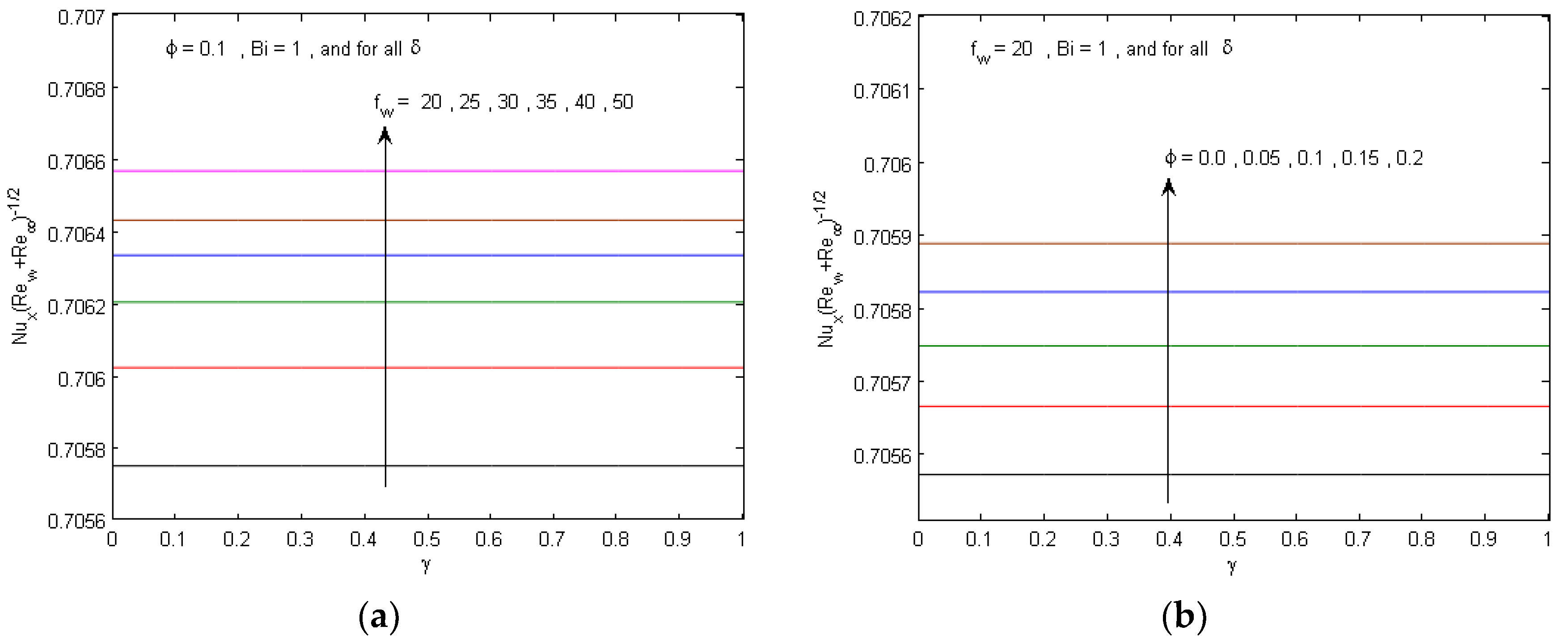
• We notice that the solutions in Equations (20) and (21) do not contain the velocity ratio parameter $\gamma$ or the slip factor $\delta$, which indicates that, for high suction, the effect of these parameters on the temperature profiles and the local Nusselt number can be neglected compared to other existing parameters.
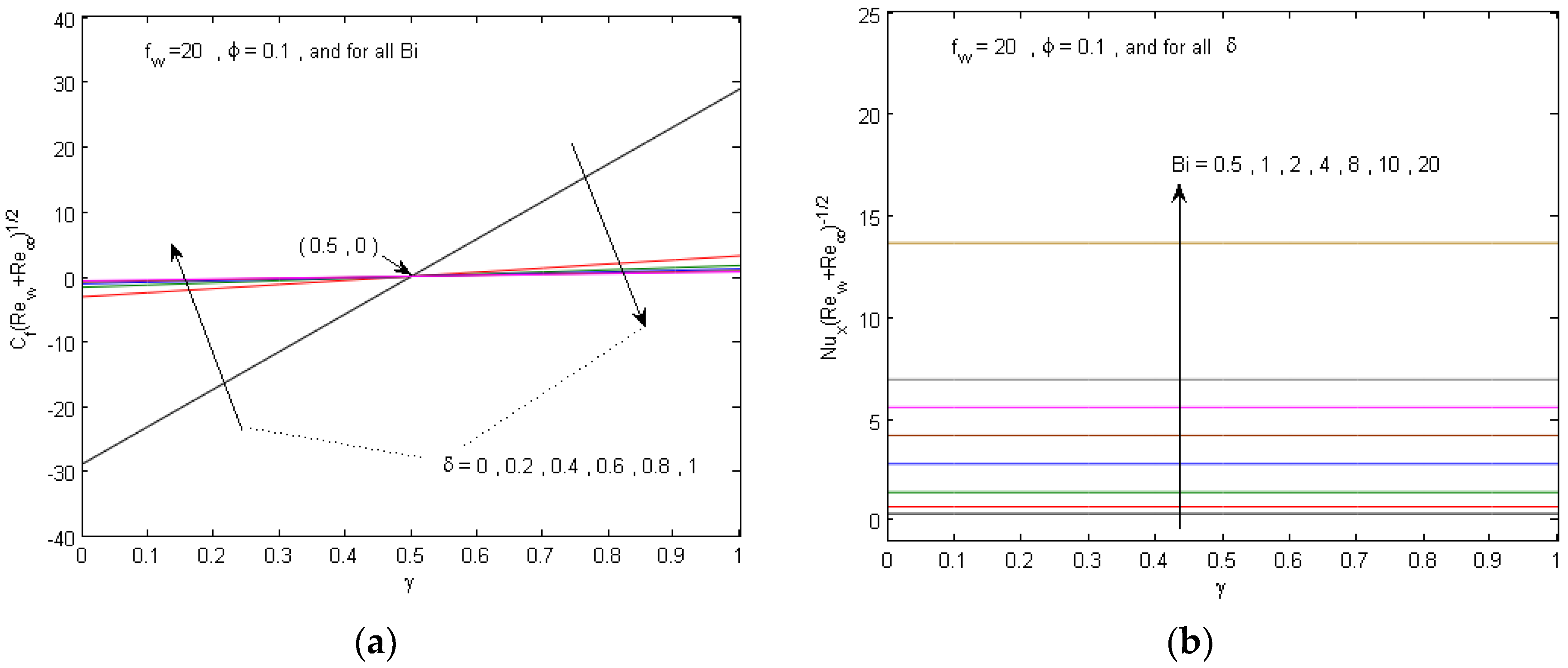
• Since we have $k_s>k_f>0$, ${(\rho C_P)}_s>{(\rho C_P)}_f>0$, and $0\le \varphi <0.5$, $k_{nf}\hspace{0.17em},\hspace{0.17em}\hspace{0.17em}\sigma >0$, and the solution in Equation (21) results in a positive local Nusselt number.
• Additionally, since we have $k_s>k_f>0$, ${(\rho C_P)}_s>{(\rho C_P)}_f>0$, and $0\le \varphi <0.5$, $k_{nf}\propto \varphi ,\hspace{0.17em}\hspace{0.17em}\hspace{0.17em}\hspace{0.17em}\hspace{0.17em}\sigma \propto \varphi \hspace{0.17em}$ and $\theta (0)\propto 1/\varphi \hspace{0.17em}$. This means that, as the solid volume fraction $\varphi$ increases the initial temperature of the wall layer, $\theta (0)$, decreases, while the thermal boundary layers thickness $O(\sigma /f_w)$ increases, which suggests that there are intersections points among $\theta (t)$ curves and the temperature profiles decrease non-monotonically.
• Moreover, the solution in Equation (20) shows that, as the suction parameter $f_w$ increases or the Biot number $Bi$ decreases, the temperature profiles decrease monotonically.
• Additionally, the solution in (21) shows that as the suction parameter $f_w$ or the Biot number $Bi$ increases the wall temperature gradients (at $\eta =0$) and the local Nusselt number increase.
• The solution in Equation (20) shows that, as the suction parameter $f_w$ increases the wall temperature and the temperature profile decrease; therefore, the thermal boundary layers thickness decreases, while the Biot number $Bi$ has a neglected effect on the temperature layer’s thickness compared to other parameters.
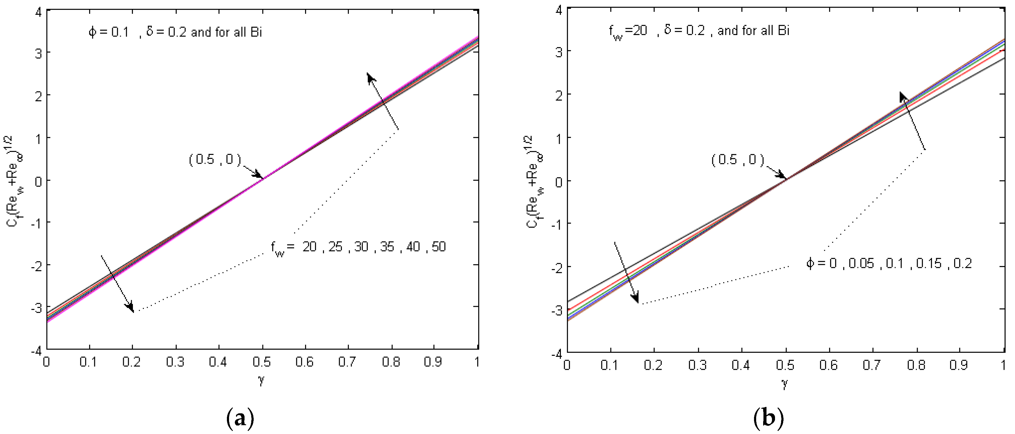
• The solutions in Equations (27)–(29) do not contain the Biot number $Bi$, which indicates that it has no effect on the fluid velocity and the Local skin friction coefficient.
• Since we have ${\rho }_s>{\rho }_f>0$ and $0\le \varphi <0.5$, $K_{\varphi }>0$, and the solution in Equation (29) always results in a negative local skin friction coefficient for $\gamma <0.5$ and a positive one for $\gamma >0.5$.
• Since we have ${\rho }_s/{\rho }_f>7/2\hspace{0.17em}$ and $\hspace{0.17em}\varphi <\frac{1-2{\rho }_s/7{\rho }_f}{1-{\rho }_s/{\rho }_f}$ $K_{\varphi }\propto \varphi$ and for $\gamma >0.5$ ($\gamma <0.5$), as the solid volume fraction parameter $\varphi$ increases, the velocity profiles decrease (increases).
• The value of $\eta$ at which $\hspace{0.17em}{f}^{\prime }(\eta )=0.5$ can be determined from Equation (27) and is given by

  $${\eta }_{f^{\prime }=0.5}=\frac{1}{k_{\varphi }{f}_w}\ln \left(\frac{2{\left(1-\varphi \right)}^{5/2}}{k_{\varphi }{f}_w\mathsf{\delta }+{\left(1-\varphi \right)}^{5/2}}\right),$$

  (32)

  which shows that, at fixed values of $f_w, \varphi$ and $\delta$, we have one intersection point $\left({\eta }_{f^{\prime }=0.5},\hspace{0.17em}\hspace{0.17em}0.5\right)$ of the velocity curves regardless of the values of $\gamma$. This intersection point lies in the right (left) half plane for $\sigma f_w<{\rho }_f/{\rho }_{nf}$ ($\sigma f_w>{\rho }_f/{\rho }_{nf}$) which confirm that for high suction, $f_w\gg 0$, and positive slip factor $\delta >0$, the intersection point lies in the left half plane.
• Moreover, based on Equations (27)–(29), for $\gamma >0.5$ ($\gamma <0.5$) and ${\overline{f}}^{″}(\eta )<0$ (${\overline{f}}^{″}(\eta )>0$), as the suction parameter $f_w$ or the slip parameter $\delta$ increases, the velocity profiles decrease (increases) monotonically.

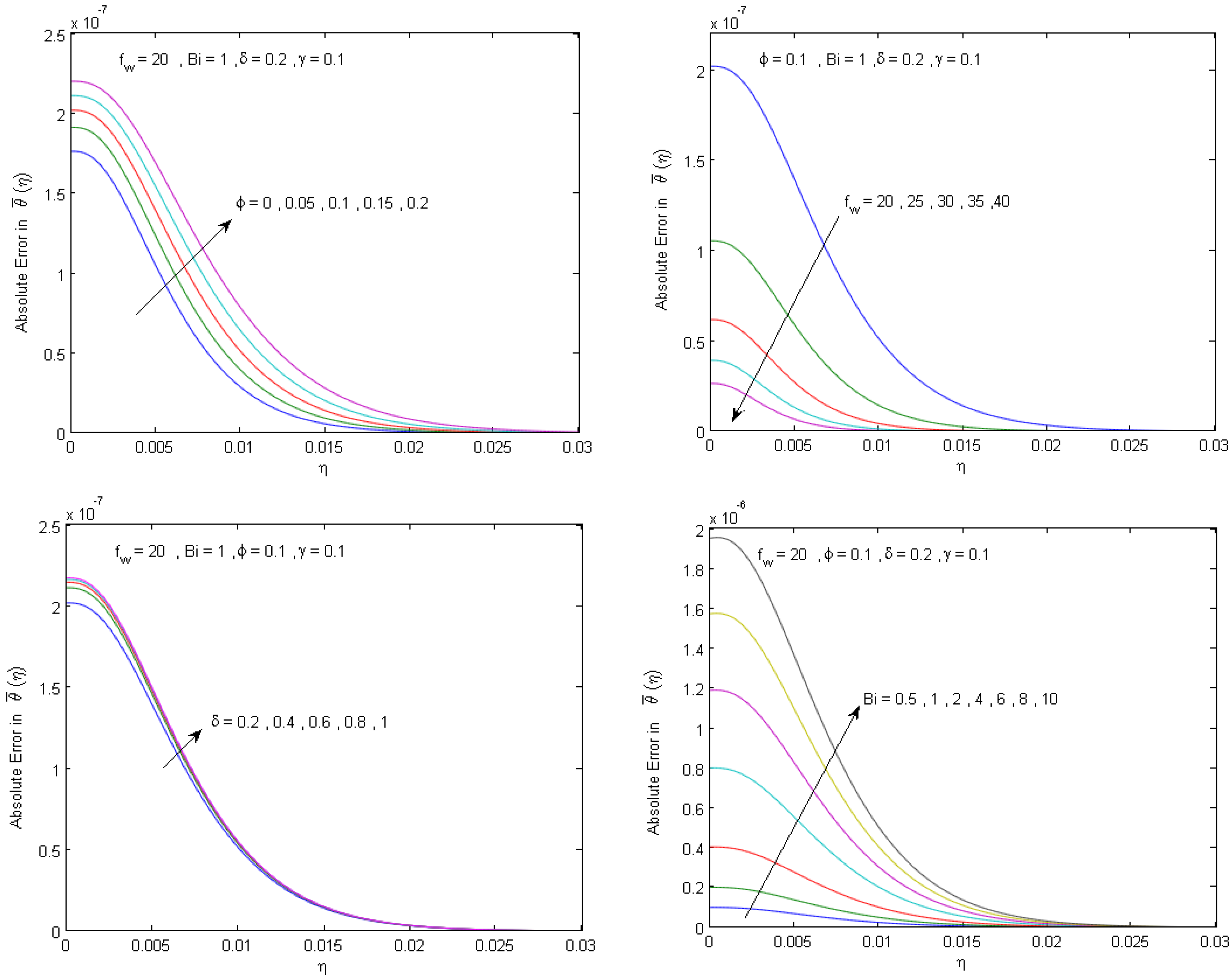
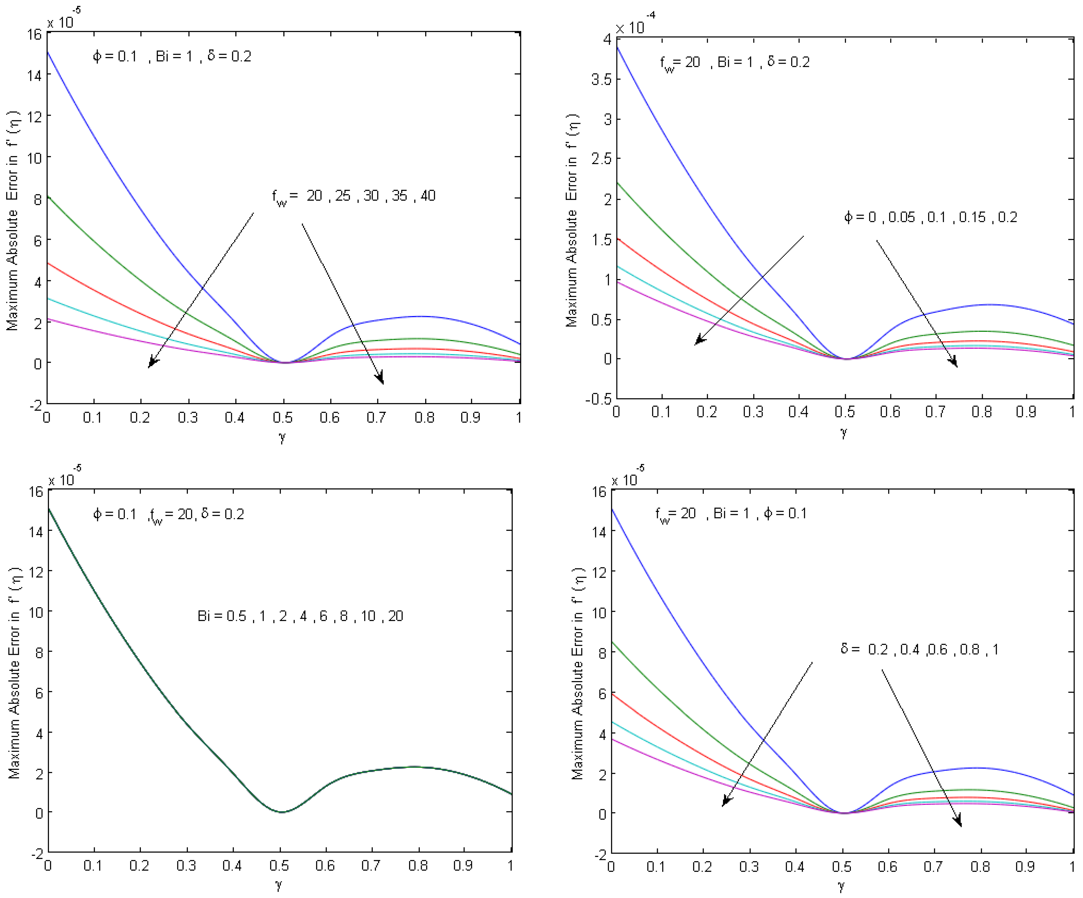
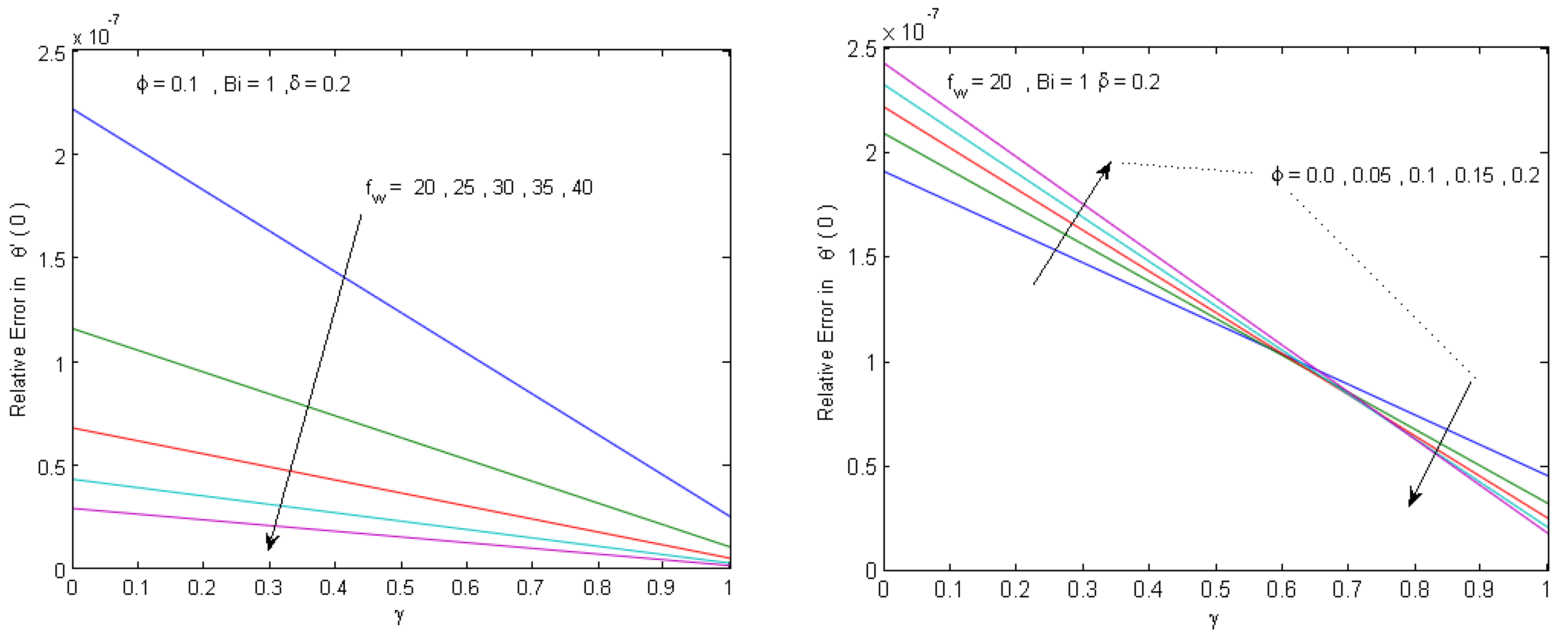
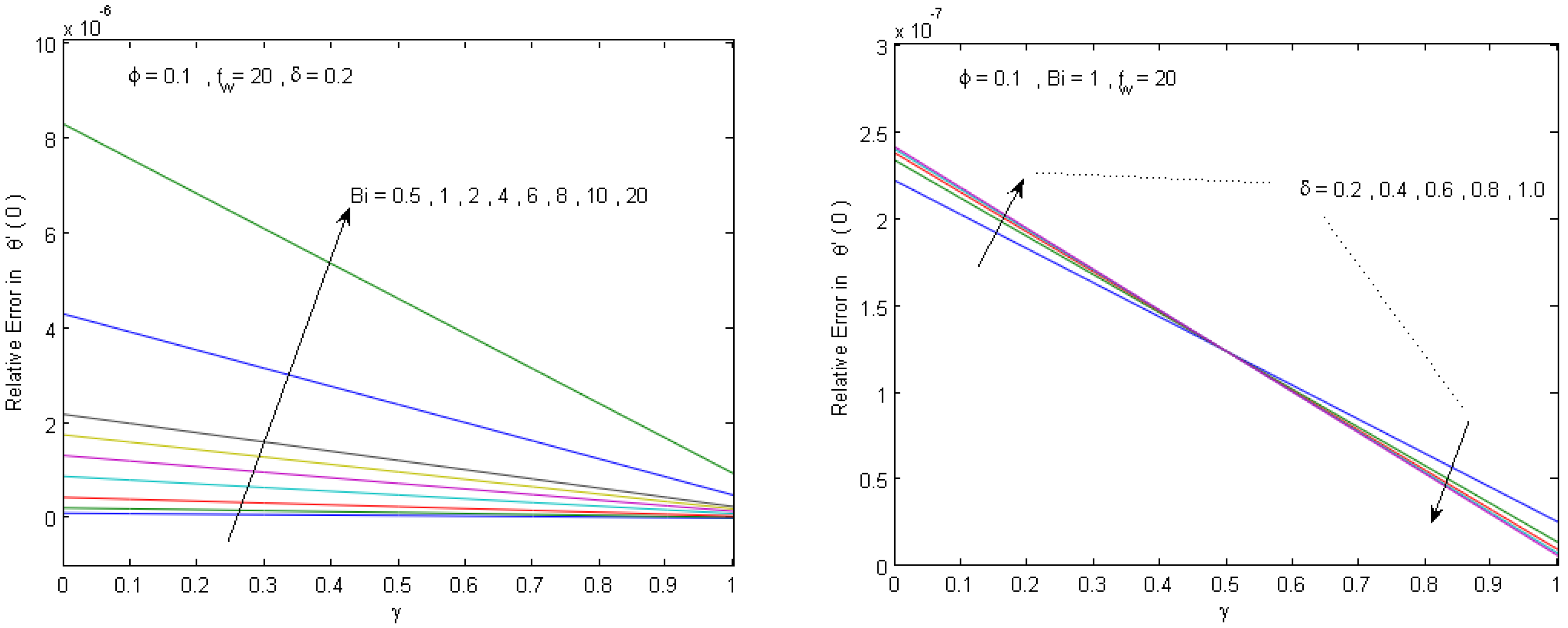
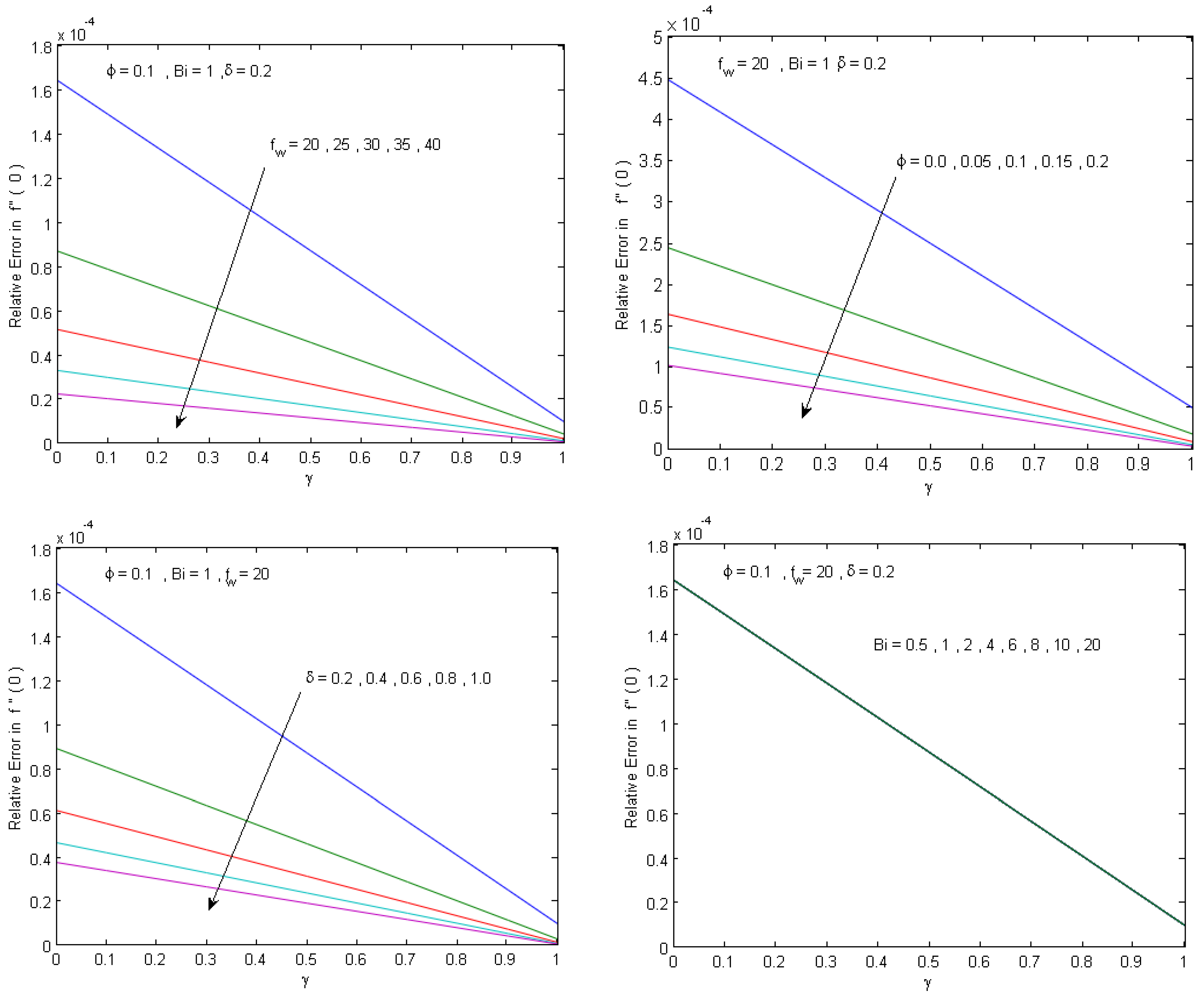
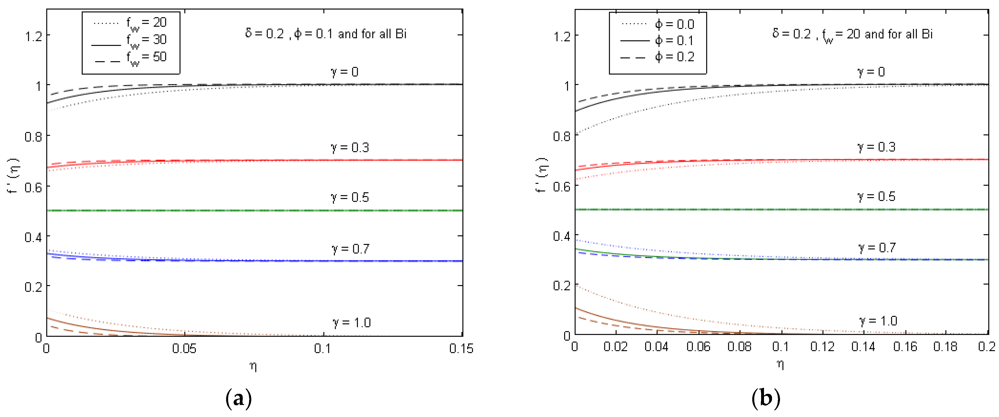
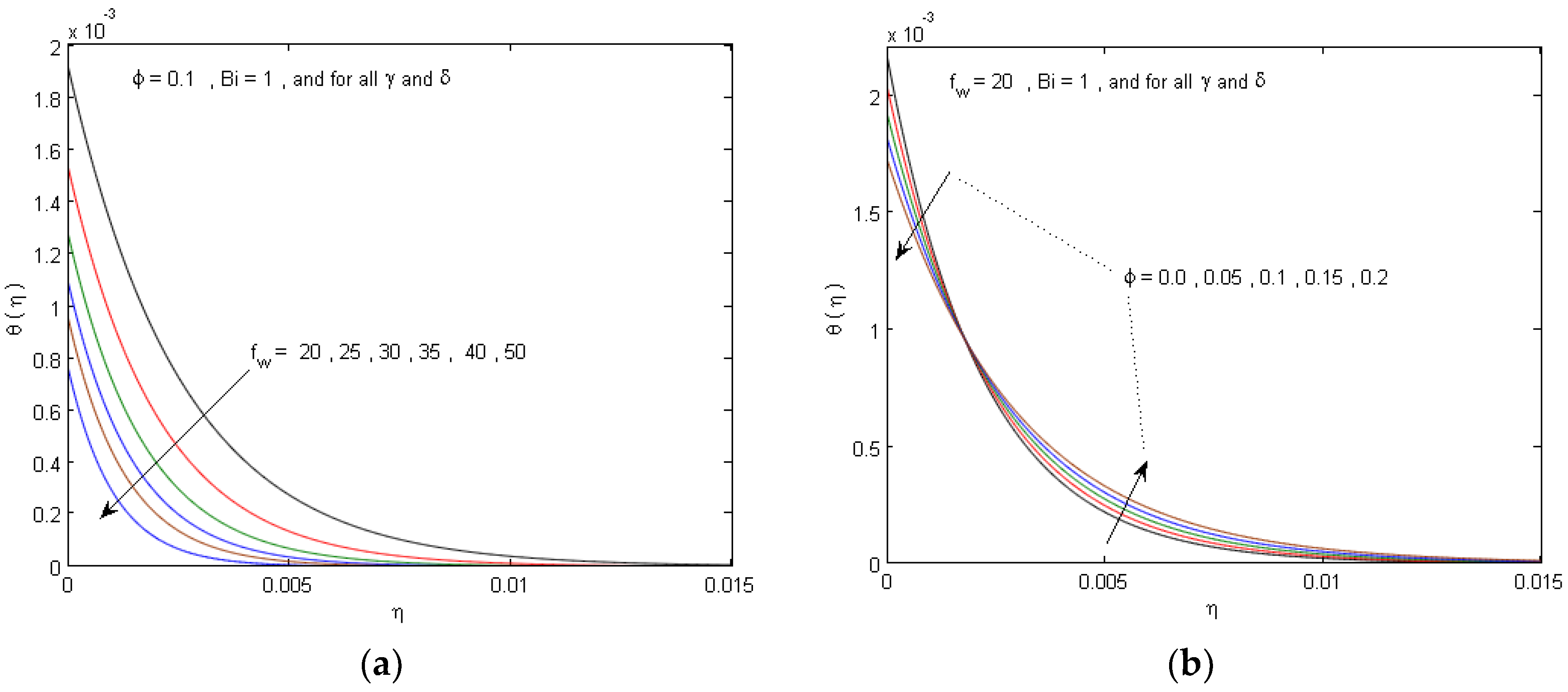
5. Numerical Results and Discussion

A numerical study was performed on the influence of solid volume fraction parameter ϕ, suction parameter f_w, slip factor δ, and Biot number Bi, with high values of suction parameter f_w, on the behavior of nanofluid velocity and temperature components as well as the local skin-friction coefficient and the local Nusselt number. The results are shown in Figure 6, Figure 7, Figure 8, Figure 9, Figure 10 and Figure 11. The present numerical study was performed for iron oxide–water nanofluid as a working fluid with various values of velocity ratio parameter γ in the range 0 ≤ γ ≤ 1. The corresponding thermo-physical properties [26] of the fluid and nanoparticles are shown in Table 1.

Figure 6 reveals the impacts of the nanoparticle volume fraction parameter ϕ and suction parameter f_w on the nanofluid velocity f’(η) and temperature profiles θ(η), respectively. The figure is limited to the status of the suction (lateral mass withdrawal over the plate surface out of the boundary layer regime). From these figures, it is manifested that velocity ratio parameter γ = 0, 0 < γ < 1, and γ = 1 coincides to a fixed plate in a movable fluid, a movable plate in a moving fluid, and a movable plate in a quiescent fluid, respectively. However, it is depicted that the imposition of a wall nanofluid suction (f_w >> 0) tends to enhance the flow along the surface, which results in increasing the velocity profiles for γ < 0.5, while the opposite can be observed for γ > 0.5. In a similar pattern, it is manifested that an increase in nanoparticle volume fraction parameter $\varphi$ causes an enhancement in the nanofluid velocity for γ < 0.5, while the opposite occurs for γ > 0.5. Additionally, both the temperature profiles and thermal boundary layer elevate constantly with the augmenting volume fraction of the nanoparticles, while the reverse occurs with the suction parameter. This coincides with the physical pattern whereby, after the volume fraction of iron oxide boosts thermal conductivity, the thermal boundary layer thickness increases, as shown in Figure 7.

Figure 8a and Figure 9b exhibit the influences of f_w and $\varphi$ on the local skin friction coefficient $C_f{\left({\mathrm{Re}}_w+{\mathrm{Re}}_{\infty }\right)}^{1/2}$ and the local Nusselt number $N{u}_x{\left({\mathrm{Re}}_w+{\mathrm{Re}}_{\infty }\right)}^{-1/2}$, respectively, with various values of γ for the parallel moving plate. It is manifested that all values of the $C_f{\left({\mathrm{Re}}_w+{\mathrm{Re}}_{\infty }\right)}^{1/2}$ are positive as γ < 0.5 and negative when γ > 0.5, while γ = 0.5 attains $C_f{\left({\mathrm{Re}}_w+{\mathrm{Re}}_{\infty }\right)}^{1/2}$ = 0, since both the fluid and plate move with the same velocity. Conversely, the values of $N{u}_x{\left({\mathrm{Re}}_w+{\mathrm{Re}}_{\infty }\right)}^{-1/2}$ are positive for all γ. For γ < 0.5, development in f_w causes a slight decline in the skin friction coefficient, while the reverse behavior can be seen for γ > 0.5. It was also noticed that the increment in ϕ has a tendency to diminish the $C_f{\left({\mathrm{Re}}_w+{\mathrm{Re}}_{\infty }\right)}^{1/2}$ as a result of the increment in the momentum thickness of the boundary layers for the status γ < 0.5, and the opposite impact is manifested for γ > 0.5. Moreover, it is evident in Figure 9a that a sufficient boosting of f_w results in an increase in $N{u}_x{\left({\mathrm{Re}}_w+{\mathrm{Re}}_{\infty }\right)}^{-1/2}$ for all γ. This conduct is related to the remarkable reduction in the thermal boundary layers as f_w boosts. However, as mentioned, the rise in volume fraction parameter $\varphi$ leads to an increase in the temperature profiles and thermal boundary layers, which results in an increase in $N{u}_x{\left({\mathrm{Re}}_w+{\mathrm{Re}}_{\infty }\right)}^{-1/2}$, as shown in Figure 9b. This is consistent with the physical manner in which the susceptibility of the thermal boundary layer thickness to $\varphi$ is concerned with the enhanced thermal conductivity of the nanofluid (see Table 1), which in turn enhances in thermal diffusivity and, consequently, following Equation (14), causes a significant evolution in the local Nusselt number.

Figure 10 demonstrates the impacts of the velocity slip parameter δ and the Biot number Bi on f’(η) and θ(η), respectively. It is apparent that an elevation in Bi leads to a salient increment in the temperature distributions. In addition, an increment in δ tends to accelerate the flow along the movable surface filled with nanofluid when γ < 0.5, while the opposite trend can be observed when γ > 0.5. Finally, the variations in skin friction coefficient and Nusselt number ($C_f{\left({\mathrm{Re}}_w+{\mathrm{Re}}_{\infty }\right)}^{1/2}$, $N{u}_x{\left({\mathrm{Re}}_w+{\mathrm{Re}}_{\infty }\right)}^{-1/2}$) versus γ, respectively, for several values of δ and Bi, respectively, are revealed in Figure 11a,b. This reason because, as Bi increases, the convective heat transfer from the hot nanofluid portion on the surface to the cold nanofluid portion rises leading to an increment in the temperature gradients. Moreover, the elevation in the slip parameter δ causes a prominent enhancement in the $C_f{\left({\mathrm{Re}}_w+{\mathrm{Re}}_{\infty }\right)}^{1/2}$ for the status γ < 0.5, whilst the behavior is reversed for γ > 0.5.

In fact, the present numerical study with results shown in Figure 6, Figure 7, Figure 8, Figure 9, Figure 10 and Figure 11 confirms a high validation of the present parametric study.

6. Conclusions

The influences of the impacts of high suction and partial slip on iron oxide nanoliquid flow over a porous moving surface in a parallel free stream with Newtonian heating is investigated analytically and numerically. The analytic solutions of the velocity function and temperature distributions are obtained via a singular perturbation technique. The bounded errors of the proposed solutions are derived through Theorems 1 and 2 and the accuracy of the proposed method is verified by comparisons between the numerical and analytical results. The solution graphs are computed and clarified for specific range of embedded parameters. Moreover, profiles of skin friction coefficient and heat transfer rate are also sketched portrayed and elaborated. The concluding remarks are specified as:

• The present singular perturbation technique results in a closed form asymptotic solution of the energy and Blasuis equations as a function of the physical parameters.
• The numerical results in Figure 2, Figure 3, Figure 4 and Figure 5 agree with theoretical ones (Theorems 1 and 2) and illustrate that the proposed technique yields a good approximation to the solution as well as the solution calculation has no CPU time-consuming or round off error.
• The rapid calculation of the system solution (dynamic response) with acceptable accuracy demonstrates that the analytical solutions are effective for performing analytical parametric studies.
• An analytical parametric study is carried out to predict the impact of the system physical parameters on the temperature and velocity behaviors.
• A numerical study is performed on the influence of the system physical parameters on the system behavior and the numerical results are present in Figure 6, Figure 7, Figure 8, Figure 9, Figure 10 and Figure 11.
• The results of the numerical study confirms a high validation of the present analytical parametric study and their main results can be summarized as follows:
  • Both the nanofluid velocity and temperature distributions are decelerated for growing the solid volume fraction and suction parameters.
  • The raising in slip parameter causes an increment in the velocity profiles, and the raising in Biot number causes an increment in the temperature profiles.
  • The local Nusselt number elevates along with boosting values of Biot number solid volume fraction and suction parameters.

References

- He, J.H. Homotopy perturbation technique. Comput. Methods Appl. Mech. Eng. 1999, 178, 257–262. [Google Scholar] [CrossRef]
- Rashidi, M.M.; Keimanesh, M. Using differential transform method and the Padé approximant for solving MHD flow in a laminar liquid film from a horizontal stretching surface. Math. Prob. Eng. 2010, 20, 14. [Google Scholar] [CrossRef]
- Shi, J.; Wang, L.; Wang, Y.; Zhang, J. Generalized energy flow analysis considering electricity gas and heat subsystems in local-area energy systems integration. Energies 2017, 10, 514. [Google Scholar] [CrossRef]
- Habib, H.M.; El-Zahar, E.R. Mathematical modeling of heat-transfer for a moving sheet in a moving fluid. J. Appl. Fluid Mech. 2013, 6, 369–373. [Google Scholar]
- El-Zahar, E.R.; Rashad, A.M.; Gelany, A.M. Studying high suction effect on boundary-layer flow of a nanofluid on permeable surface via singular perturbation technique. J. Comput. Theoret. Nanosci. 2015, 12, 4828–4836. [Google Scholar] [CrossRef]
- Sakiadis, B.C. Boundary layers on continuous solid surfaces. AIChE J. 1961, 7, 26–28, 221–225, 467–472. [Google Scholar] [CrossRef]
- Crane, L.J. Flow past a stretching plane. ZAMP 1970, 21, 645–647. [Google Scholar]
- Tsou, F.; Sparrow, E.; Goldstein, R. Flow and heat transfer in the boundary layer on a continuous moving surface. Int. J. Heat Mass Transf. 1967, 10, 219–235. [Google Scholar] [CrossRef]
- Magyari, E.; Keller, B. Heat and mass transfer in the boundary layers on an exponentially stretching continuous surface. J. Phys. D: Appl. Phys. 1999, 32, 577–585. [Google Scholar] [CrossRef]
- Magyari, E.; Keller, B. Exact solutions for self-similar boundary-layer flows induced by permeable stretching walls. Eur. J. Mech. B/Fluids. 2000, 19, 109–122. [Google Scholar] [CrossRef]
- El-Kabeir, S.M.M.; Rashad, A.M.; Gorla, R.S.R. Unsteady MHD combined convection over a moving vertical sheet in a fluid saturated porous medium with uniform surface heat flux. Math. Comput. Model. 2007, 46, 384–397. [Google Scholar] [CrossRef]
- Bataller, R.C. Radiation effects in the blasius flow. Appl. Math. Comput. 2008, 198, 333–338. [Google Scholar]
- Ishak, A. Radiation effects on the flow and heat transfer over a moving plate in a parallel stream. Chin. Phys. Lett. 2009, 26, 034701. [Google Scholar] [CrossRef]
- El-Kabeir, S.M.M.; El-Hakiem, M.A.; Rashad, A.M. Lie group analysis of unsteady MHD three dimensional by natural convection from an inclined stretching surface saturated porous medium. J. Comput. Appl. Math. 2008, 213, 582–603. [Google Scholar] [CrossRef] [Green Version]
- Rashad, A.M.; Bakier, A.Y.; Gorla, R.S.R. Viscous dissipation and ohmic heating effects on MHD mixed convection along a vertical moving surface embedded in a fluid saturated porous medium. J. Porous Med. 2010, 13, 159–170. [Google Scholar] [CrossRef]
- El-Kabeir, S.M.M.; Rashad, A.M.; Gorla, R.S.R. Heat transfer in a micropolar fluid flow past a permeable continuous moving surface. ZAMM 2011, 91, 1–11. [Google Scholar] [CrossRef]
- Choi, S.U.S.; Eastman, J.A. Enhancing thermal conductivity of fluids with nanoparticles. In Proceedings of the ASME International Mechanical Engineering Congress and Exposition, San Francisco, CA, USA, 12–17 November 1995; Volume 231, pp. 99–103. [Google Scholar]
- Buongiorno, J. Convective transport in nanofluids. ASME J. Heat Transf. 2006, 128, 240–250. [Google Scholar] [CrossRef]
- Chamkha, A.J.; Rashad, A.M.; Al-Meshaiei, E. Melting effect on unsteady hydromagnetic flow of a nanofluid past a stretching sheet. Int. J. Chem. React. Eng. 2011, 9, 1–23. [Google Scholar] [CrossRef]
- Rashad, A.M.; El-Hakiem, M.A.; Abdou, M.M.M. Natural convection boundary layer of a non-Newtonian fluid about a permeable vertical cone embedded in a porous medium saturated with a nanofluid. Comput. Math. Appl. 2011, 62, 3140–3151. [Google Scholar] [CrossRef] [Green Version]
- Chamkha, A.J.; Rashad, A.M. Natural convection from a vertical permeable cone in nanofluid saturated porous media for uniform heat and nanoparticles volume fraction fluxes. Int. J. Numer. Method. Heat Fluid Flow. 2012, 22, 1073–1085. [Google Scholar] [CrossRef]
- Bég, O.A.; Ferdows, M. Explicit numerical simulation of magnetohydrodynamic nanofluid flow from an exponential stretching sheet in porous media. Appl. Nanosci. 2013, 1–15. [Google Scholar] [CrossRef]
- Chamkha, A.J.; Rashad, A.M.; Aly, A.M. Transient natural convection flow of a nanofluid over a vertical cylinder. Meccanica 2013, 48, 71–81. [Google Scholar] [CrossRef]
- Noghrehabadi, A.; Behseresht, A.; Ghalambaz, M.; Behseresht, J. Natural convection flow of nano fluids over a vertical cone embedded in a non-Darcy porous medium. J. Thermophys. Heat Transf. 2013, 27, 334–341. [Google Scholar] [CrossRef]
- Behseresht, A.; Noghrehabadi, A.; Ghalambaz, M. Natural convection heat and mass transfer from a vertical cone in porous media filled with nano fluids using the practical ranges of nano fluids thermophysical properties. Chem. Eng. Res. Des. 2014, 92, 447–452. [Google Scholar] [CrossRef]
- Rashad, A.M.; Abbasbandy, S.; Chamkha, A.J. Non-Darcy natural convection from a vertical cylinder embedded in a thermally stratified and nanofluid-saturated porous media. ASME J. Heat Transf. 2014, 136, 002503. [Google Scholar] [CrossRef]
- Choi, S.U.S. Enhancing thermal conductivity of fluids with nanoparticle. In Developments and Applications of Non-Newtonian Flows, Proceedings of the ASME FED International Mechanical Engineering Congress & Exposition, San Francisco, CA, USA, 12–17 November 1995; Siginer, D.A., Wang, H.P., Eds.; US Department of Energy, Basic Energy Sciences-Material Sciences: Washington, DC, USA, 1995; Volume 231, pp. 99–105. [Google Scholar]
- Tiwari, R.K.; Das, M.K. Heat transfer augmentation in a two-sided lid-driven differentially heated square cavity utilizing nanofluids. Int. J. Heat Mass Tran. 2007, 50, 2002–2018. [Google Scholar] [CrossRef]
- El-Kabeir, S.M.M.; Chamkha, A.J.; Rashad, A.M. The effect of thermal radiation on non-Darcy free convection from a vertical cylinder embedded in a nanofluid porous media. J. Porous Med. 2014, 17, 269–278. [Google Scholar] [CrossRef]
- El-Kabeir, S.M.M.; Modather, M.; Rashad, A.M. Effect of thermal radiation on mixed convection flow of a nanofluid about a solid sphere in a saturated porous medium under convective boundary condition. J. Porous Med. 2015, 18, 569–584. [Google Scholar] [CrossRef]
- Rashad, A.M. Impact of thermal radiation on MHD slip flow of a ferrofluid over a nonisothermal wedge. J. Magn. Mater. 2017, 422, 25–31. [Google Scholar] [CrossRef]
- Rashad, A.M. Unsteady nanofluid flow over an inclined stretching surface with convective boundary condition and anisotropic slip impact. Int. J. Heat Technol. 2017, 35, 82–90. [Google Scholar] [CrossRef]
- Bhatti, M.M.; Abbas, T.; Rashidi, M.M.; Ali, M.E.; Yang, Z. Entropy generation on MHD eyring—Powell nanofluid through a permeable stretching surface. Entropy 2016, 18, 224. [Google Scholar] [CrossRef]
- Garoosi, F.; Hoseininejad, F.; Rashidi, M.M. Numerical study of heat transfer performance of nanofluids in a heat exchanger. Appl. Therm. Eng. 2016, 105, 436–455. [Google Scholar] [CrossRef]
- Khalili, S.; Tamim, H.; Khalili, A.; Rashidi, M.M. Unsteady convective heat and mass transfer in pseudoplastic nanofluid over a stretching wall. Adv. Powder Technol. 2015, 26, 1319–1326. [Google Scholar] [CrossRef]
- Bashirnezhad, K.; Rashidi, M.M.; Yang, Z.; Bazri, S.; Yan, W.M. A comprehensive review of last experimental studies on thermal conductivity of nanofluids. J. Therm. Anal. Calorim. 2014, 9, 863–884. [Google Scholar] [CrossRef]
- Mohebbi, R.; Rashidi, M.M. Numerical simulation of natural convection heat transfer of a nanofluid in an L-shaped enclosure with a heating obstacle. J. Taiwan Instit. Chem. Eng. 2017, 72, 70–84. [Google Scholar] [CrossRef]
- Li, Y.; Yan, H.; Massoudi, M.; Wu, W.T. Effects of anisotropic thermal conductivity and Lorentz force on the flow and heat transfer of a ferro-nanofluid in a magnetic field. Energies 2017, 10, 1065. [Google Scholar] [CrossRef]
- Salleh, S.N.A.; Bachok, N.; Arifin, N.M.; Ali, F.M.; Pop, I. Magnetohydrodynamics flow past a moving vertical thin needle in a nanofluid with stability analysis. Energies 2018, 11, 3297. [Google Scholar] [CrossRef]
- O’Malley, R.E. Introduction to Singular Perturbations; Academic Press: New York, NY, USA, 1974. [Google Scholar]
- Bender, C.M.; Orszag, S.A. Advanced Mathematical Methods for Scientists and Engineers, International Series in Pure and Applied Mathematic; McGraw-Hill: New York, NY, USA, 1978. [Google Scholar]
- Doolan, E.P.; Miller, J.J.H.; Schilders, W.H.A. Uniform Numerical Methods for Problems with Initial and Boundary Layers; Boole Press: Dublin, Ireland, 1980. [Google Scholar]
- Kadalbajoo, M.K.; Patidar, K.C. A survey of numerical techniques for solving singularly perturbed ordinary differential equations. Appl. Math. Comput. 2002, 130, 457–510. [Google Scholar] [CrossRef]
- Kumar, M.; Singh, P.; Mishra, H.K. A recent survey on computational techniques for solving singularly perturbed boundary value problems. Int. J. Comput. Math. 2007, 84, 1–25. [Google Scholar] [CrossRef]
- Miller, J.J.; O’Riordan, E.; Shishkin, G.I. Fitted Numerical Methods for Singular Perturbation Problems: Error Estimates in the Maximum Norm for Linear Problems in One and Two Dimensions; World Scientific: Singapore, 2012. [Google Scholar]
- Verhulst, F. Methods and Applications of Singular Perturbations: Boundary Layers and Multiple Timescale Dynamics; Springer Science and Business Media: Berlin, Germany, 2006. [Google Scholar]
- Ross, H.G.; Stynes, M.; Tobiska, L. Robust Numerical Methods for Singularly Perturbed Differential Equations: Convection-Diffusion-Reaction and Flow Problems; Springer Science & Business Media: Berlin, Germany, 2008; Volume 24. [Google Scholar]
- Habib, H.M.; El-Zahar, E.R. Variable step size initial value algorithm for singular perturbation problems using locally exact integration. Appl. Math. Comput. 2008, 200, 330–340. [Google Scholar] [CrossRef]
- El-Zahar, E.R.; EL-Kabeir, S.M.M. A new method for solving singularly perturbed boundary value problems. Appl. Math. Inf. Sci. 2013, 7, 927–938. [Google Scholar] [CrossRef]
- Vulanovic, R. A uniform numerical method for quasilinear singular perturbation problems without turning points. Computing 1989, 41, 97–106. [Google Scholar] [CrossRef]
- Kierzenka, J.; Shampine, L.F. A BVP solver based on residual control and the MATLAB PSE. ACM Trans. Math. Softw. 2001, 27, 299–316. [Google Scholar] [CrossRef]
© 2019 by the authors. Licensee MDPI, Basel, Switzerland. This article is an open access article distributed under the terms and conditions of the Creative Commons Attribution (CC BY) license (http://creativecommons.org/licenses/by/4.0/).
Share and Cite
Chamkha, A.J.; Rashad, A.M.; EL-Zahar, E.R.; EL-Mky, H.A. Analytical and Numerical Investigation of Fe3O4–Water Nanofluid Flow over a Moveable Plane in a Parallel Stream with High Suction. Energies 2019, 12, 198. https://doi.org/10.3390/en12010198
Chamkha AJ, Rashad AM, EL-Zahar ER, EL-Mky HA. Analytical and Numerical Investigation of Fe3O4–Water Nanofluid Flow over a Moveable Plane in a Parallel Stream with High Suction. Energies. 2019; 12(1):198. https://doi.org/10.3390/en12010198
Chicago/Turabian StyleChamkha, A. J., A. M. Rashad, E. R. EL-Zahar, and Hamed A. EL-Mky. 2019. "Analytical and Numerical Investigation of Fe3O4–Water Nanofluid Flow over a Moveable Plane in a Parallel Stream with High Suction" Energies 12, no. 1: 198. https://doi.org/10.3390/en12010198