Integration Capability Evaluation of Wind and Photovoltaic Generation in Power Systems Based on Temporal and Spatial Correlations

Abstract

With the rapid growth of renewable energy generation, it has become essential to give a comprehensive evaluation of renewable energy integration capability in power systems to reduce renewable generation curtailment. Existing research has not considered the correlations between wind power and photovoltaic (PV) power. In this paper, temporal and spatial correlations among different renewable generations are utilized to evaluate the integration capability of power systems based on the copula model. Firstly, the temporal and spatial correlation between wind and PV power generation is analyzed. Secondly, the temporal and spatial distribution model of both wind and PV power generation output is formulated based on the copula model. Thirdly, aggregated generation output scenarios of wind and PV power are generated. Fourthly, wind and PV power scenarios are utilized in an optimal power flow calculation model of power systems. Lastly, the integration capacity of wind power and PV power is shown to be able to be evaluated by satisfying the reliability of power system operation. Simulation results of a modified IEEE RTS-24 bus system indicate that the integration capability of renewable energy generation in power systems can be comprehensively evaluated based on the temporal and spatial correlations of renewable energy generation.

1. Introduction

To cope with the impending fossil energy crisis, environmental pollution, and the greenhouse effect, renewable energy is being developed rapidly, especially with regards to power generation. Given the superiorities of clean energy and its low marginal price, renewable energy generation, including wind power and photovoltaic (PV) power, has occupied a larger and larger proportion of power system generation in recent years. While the global cumulative installed capacity of wind power in 2008 amounted to only 120.8 GW, the following decade saw a rapid growth rate and the number was predicted to reach 592 GW in 2018 [1]. There is also currently a distinct global development in PV generation. With a total installed capacity of 15.84 GW in 2008, it was forecast to total 501.6 GW in 2018 [2].

However, the generation outputs of wind turbines and PV panels depend heavily on the weather, which leads to the nondeterministic nature of wind power and PV power. For example, wind power generation relies largely on the wind speed and wind direction [3], while solar irradiance and ambient temperature are the key factors affecting PV power [4]. Due to the inherent uncertainty of wind and PV power, it is difficult to make full use of these renewable generations. In addition, most existing power system networks were designed and built years ago without enough foresight to imagine such rapid growth in renewable generation [5,6]. Moreover, most renewable generation farms are built at the end of power grids. Existing factors, such as transmission capacities and reserve capacities, constrain the capability of power systems from fully adopting renewable generation, thereby resulting in severe wind power and PV power curtailments [7]. Therefore, it is essential to evaluate the integration capability of renewable energy generation in power systems, which can be utilized in power system planning for updating networks or building new renewable generation farms.

Much research has been done on evaluating the integration capacity of either wind power or PV power generation in power systems [8]. The impact of increasing PV penetration on the static performance and transient stability of transmission systems was analyzed in [9]. In [10], optimal levels of plug-in electric vehicles and renewable distributed generation penetration with respect to the location, size, and year of installation were optimized based on a non-dominated sorting genetic algorithm. Technologies for accommodating renewable resources penetration have been proposed in cooperation with energy storage systems and grid flexibility [11,12]. Distribution system feeders have also been investigated to cope with the possible voltage problems related to the integration sizes and locations of PV generation and loads [13]. The flexibility requirements for wind and solar power in Europe were quantitatively evaluated in terms of ramping capability and geography in [14]. Voltage source inverters control strategies in renewable energy integration in power systems have also been widely studied [15]. A comprehensive review for analysis of renewable energy integration into multi-energy systems was presented in [16]. However, most existing research either focuses on penetration capability analysis with individual renewable resources or combinations of multiple renewable resources without considering their correlations in time and space. It is possible for outputs of wind generation and PV generation to have large temporal and spatial correlations because of their shared dependence on weather forecasts. This correlation may distort the aggregated outputs of wind power and PV power compared with their direct summation results. The correlation between wind and PV power has been explored in a number of studies. For example, the sample correlation coefficient between wind and PV power was calculated in [17]. In [18], a Monte Carlo based method was adopted for the assessment of wind and PV power correlations. However, the joint probability distribution of wind and solar power has not been formulated in these studies. Without distribution estimations, it is difficult to take wind and PV power correlations into account in evaluating renewable generation penetration in power system planning.

In this paper, a novel approach for evaluating the integration capability of renewable energy generation in transmission systems is proposed based on temporal and spatial correlations. Firstly, the correlations between wind and PV power series in different time periods and locations are analyzed based on the cross-correlation function (CCF). Secondly, an aggregated generation output distribution model of wind and PV power is formulated from individual predictive distributions based on the copula function. In addition, aggregated generation outputs are segmented based on different correlation degrees of wind and PV power series. Thirdly, an optimization model with the objective of maximizing the loss of load probability (LOLP) index is established based on the aggregated renewable generation distribution corresponding to the varying installed capacities of wind farms and PV power farms. Lastly, the optimal installed capacities of wind power and PV power is shown to be able to be achieved by solving the optimization model.

2. Aggregated Renewable Generation Model Based on the Copula Function

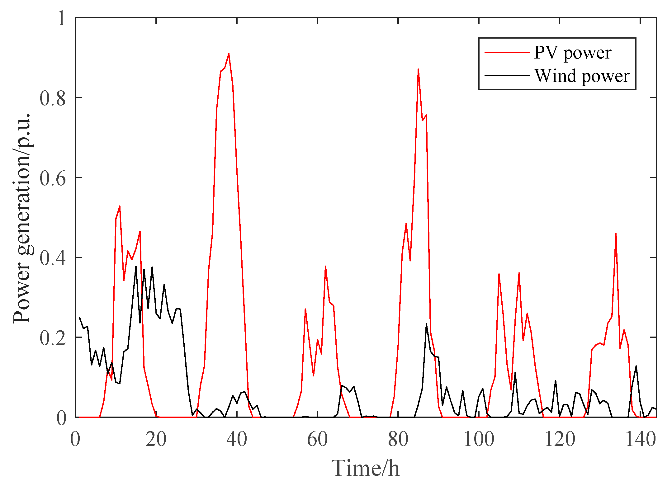
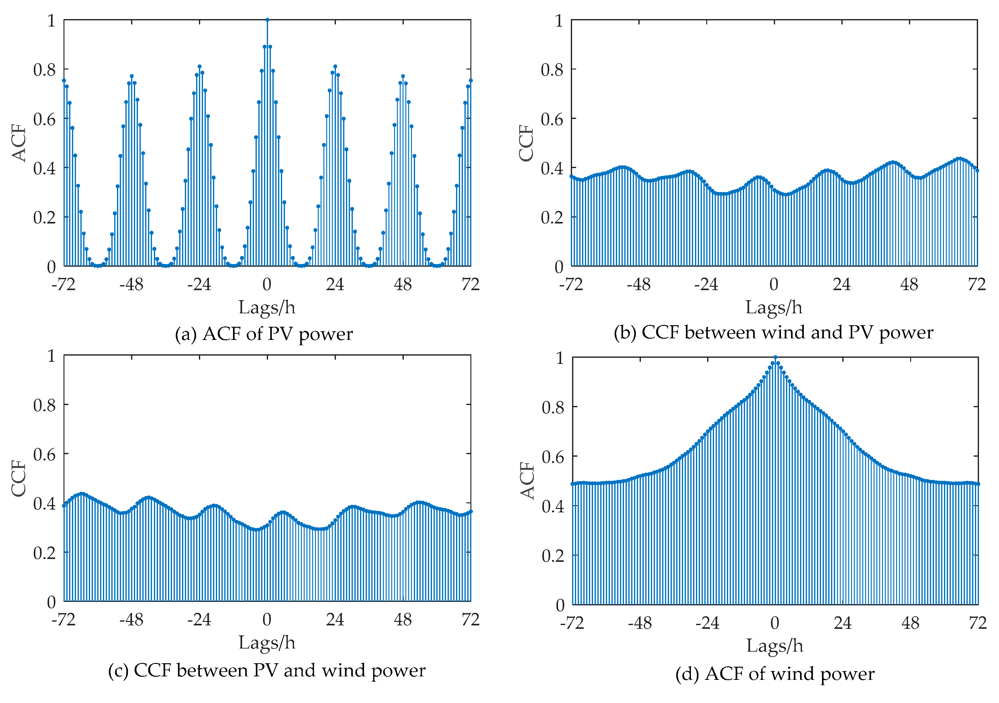
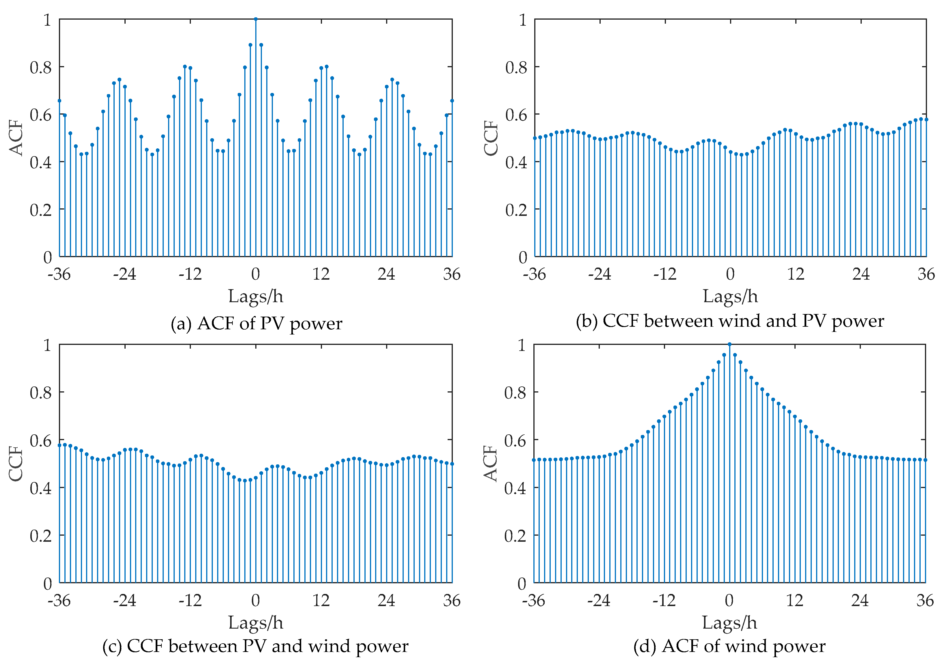
2.1. Correlation Analysis

A correlation analysis is critical for estimating the probability of renewable energy power output and determining a reasonable strategy of renewable energy generation aggregation. The statistical properties of wind power and PV power series are explained in this section.

To intuitively present the correlations between wind power and PV power, the different time series of normalized wind power generation and PV power generation are shown in Figure 1. The wind farm and PV farm shown in this figure are from the same area. It is clearly shown in this figure that wind power and PV power are correlated in some degree when in the same area.

To give a mathematical description of the correlations between wind power and PV power, we adopt the Auto-Correlation Function (ACF) and the Cross-Correlation Function (CCF) [19] to explore the temporal and spatial dependence of wind power and PV power. Given a set of sampled wind power and PV power series, the ACF of wind power and PV power series can be defined as

$$\rho \left(a\right)=\frac{\mathrm{E}\left[\left(g_t-\mu \right)\left(g_{t-a}-\mu \right)\right]}{{\sigma }^2}$$

(1)

where a is the lag time between the two series; $g_t$ is the power generation of the PV or wind farm at time t; and $\mu$ and ${\sigma }^2$ are the mean value and variance of the time series, respectively.

The CCF between two times series is defined as

$${\rho }_{i,j}\left(a\right)=\frac{\mathrm{E}\left[\left(g_{pv,i,t}-{\mu }_i\right)\cdot \left(g_{wind,j,t-a}-{\mu }_j\right)\right]}{{\sigma }_i\cdot {\sigma }_j}$$

(2)

where $g_{pv,i,t}$ and $g_{wind,j,t-a}$ are the power of sampled PV series $i$ and sampled wind power series $j$ at time t, respectively; a is the lag time between the two series; ${\mu }_i$ and ${\sigma }_i$ are the mean value and variance of sampled PV series $i$, respectively; and ${\mu }_j$ and ${\sigma }_j$ are the mean value and variance of sampled PV series $j$, respectively.

The ACF of the PV and wind power generation, as well as the CCF values between the series of the PV farm and wind farm are presented in Figure 2. Figure 2a,d show that PV power and wind power have strong temporal dependence while PV power also has strong auto-correlation at the same time for neighboring days. Figure 2b,c show relatively large CCF values, which verifies the strong spatial dependence relation between the generation output series of wind power and PV power in the same area. However, as shown in Figure 1, PV power output at night is zero, which may reduce the cross-correlation between PV and wind power. For this reason, we tested the CCF values between PV and wind power by removing the time segments when PV output was zero in both the PV and wind power series. The results are shown in Figure 3, which indicates that the spatial dependence between PV and wind farms is more obvious. Because of this, the aggregated distribution of the output of PV farms and wind farms has only been modeled for day time periods.

The spot forecasts of PV power and wind power were achieved based on the Sparse Bayesian Learning (SBL) model. SBL is a parametric forecasting method that assumes wind power and PV power output follow Gaussian distributions. Although the statistical distributions of power generation time series are non-Gaussian, some research has verified its effectiveness in modeling the uncertainty characteristics of renewable generation [20]. In this paper, we only utilize the SBL model to forecast the expectations of wind power and PV power. It should be noted that any forecasting method which has good forecasting accuracy can be utilized to obtain spot forecast results of wind and PV power in this model. Thus, the forecast error series of PV power and wind power can be calculated by a comparison with the real measurements of PV power and wind power.

In addition, cross-correlation between the PV forecast error and wind forecast error series was tested. The results show significant cross-correlation relationships. Therefore, the PV forecast error and wind forecast error series have been utilized in the power aggregation model.

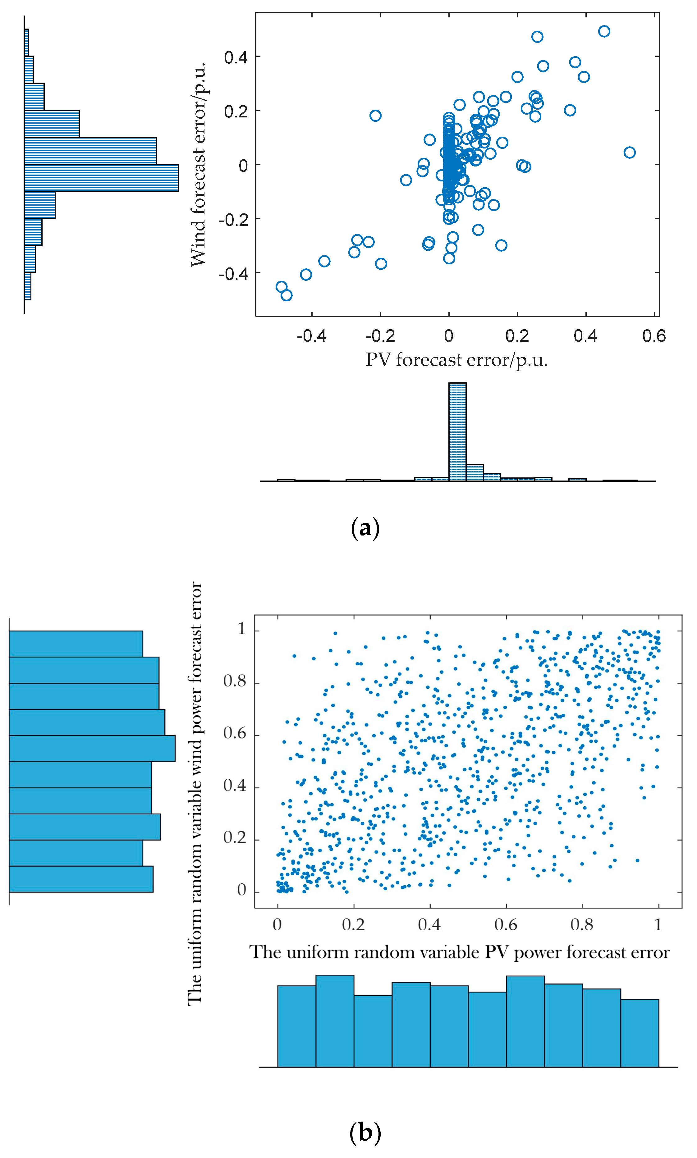
2.2. Aggregated Generation Distribution of Wind Power and PV Power Based on the Copula Function

2.2.1. Basics of the Copula Function

The copula function is a function widely utilized for calculating the joint distributions of random variables given all marginal distributions [21]. A bivariate copula function can be described as

$$F\left(e_{pv},e_{wind}\right)=C\left(F_{pv}\left(e_{pv}\right),F_{wind}\left(e_{wind}\right)\right)$$

(3)

where C(·) represents the copula function; $F_{pv}(\cdot )$ and $F_{wind}(\cdot )$ are the marginal cumulative distribution functions (CDFs) of PV and wind power, respectively; $e_{pv}$ and $e_{wind}$ stand for the random variables of PV and wind power forecast errors, respectively; and F(·) is the joint CDF of the random variables, that is, in this case it is the joint CDF of PV and wind power.

Based on Sklar’s theorem [22], a unique copula function C(·) can be calculated from its continuous marginal CDFs. Therefore, in this paper, the dependence structure of wind power and PV power forecast errors may be modeled based on an appropriate copula function.

2.2.2. Copula-Based Renewable Generation Aggregation

A Gaussian copula function has been utilized in this paper. As copula functions construct the joint CDF only for uniform random variables, it is necessary to transform the marginal CDFs of wind and PV power into uniform distributions. It is indicated in [23] that for uniform random variables with a symmetrical dependence structure, a Gaussian copula function can estimate their joint CDF with high accuracy. For this reason, a scatter plot was utilized to explore the dependence structure of wind and PV power after uniform transformation. Figure 4 presents the scatter plot results of the pairs of PV and wind power forecast errors, which were obtained by calculating the difference between the sampled data and the results of the SBL prediction model mentioned in Section 2.1. In Figure 4a, the wind power and PV power forecast error series are plotted. In Figure 4b, the scatter plot of the transformed uniform random variables of wind power and PV power forecast error series are displayed. The transformation was implemented by probability integral transform rules [24]. With regards to the scatter plot results, the clearly symmetrical dependence structure demonstrates that the dependence relation between PV and wind power forecast error series can be modeled by a Gaussian copula function.

Because of this, the dependence relationship between the forecast error series of wind power and PV power was modeled by the two-dimensional Gaussian copula (as defined by [23])

$$\begin{array}{l}F\left(e_{pv},e_{wind};R\right)=C\left(F_{pv}\left(e_{pv}\right),F_{wind}\left(e_{wind}\right);R\right)\\ ={\mathsf{\Phi }}_R\left({\mathsf{\Phi }}^{-1}\left(F_{pv}\left(e_{pv}\right)\right),{\mathsf{\Phi }}^{-1}\left(F_{wind}\left(e_{wind}\right)\right)\right)\end{array}$$

(4)

where $\mathsf{\Phi }$ represents a univariate standard Gaussian CDF with ${\mathsf{\Phi }}^{-1}$ as its inverse function; and ${\mathsf{\Phi }}_R$ stands for a bivariate Gaussian joint CDF with zero means and unit marginal variances whose covariance matrix is R.

To obtain the joint CDF described in (4), the marginal CDFs of the forecast error series of wind power and PV power, as well as the corresponding correlation matrix R, must be calculated. In this paper, the marginal CDFs of the forecast error series were obtained based on the empirical CDF. R can be determined based on the maximum likelihood estimation [25]

$$\begin{array}{l}R=\arg \underset{R}{\max }{\displaystyle \prod _{i=1}^{V}c(F_{pv}\left(e_{pv,i}\right),F_{wind}\left(e_{wind,i}\right),R)}\\ =\arg \underset{R}{\max }{\displaystyle \sum _{i=1}^V\ln c(F_{pv}\left(e_{pv,i}\right),F_{wind}\left(e_{wind,i}\right),R)}\end{array}$$

(5)

where $c(\cdot )$ is the joint density function corresponding to $C(\cdot )$; V is the number of the sampled pairs of PV and wind power forecast errors and $\{e_{pv,i},e_{wind,i}\}$ is the $i^{th}$ pair. It can be seen that R calculated by (5) maximizes the probability of the occurrence of the sampled data, which is a reasonable estimation of the parameters of the Gaussian joint CDF.

According to the spot forecast results, a CDF of the spot forecast error, and the correlation matrix of the errors, V groups of the formulated two-dimensional scenarios of the aggregated output of wind power and PV power can be generated. The process is as follows:

• Step 1: Sample V groups of the two-dimensional uniform random variables PV and wind power forecast errors based on the joint CDF estimated by the Gaussian copula model in (4). The groups of these samples can be represented by ${\mathit{u}}_i=\left\{u_{pv,i},u_{wind,i}\right\},i=1,\cdots V$.
• Step 2: Transform the above V groups of sample ${\mathit{u}}_i=\left\{u_{pv,i},u_{wind,i}\right\},i=1,\cdots V$ to V groups of error samples $e_i=\left\{e_{pv,i},e_{wind,i}\right\},i=1,\cdots V$ through the inverse transformation

  $$\left\{e_{pv,i},e_{wind,i}\right\}=\left\{F_{pv}^{-1}\left(u_{pv,i}\right),F_{wind}^{-1}\left(u_{wind,i}\right)\right\}$$

  (6)

  where $F_{pv}^{-1}(\cdot )$ and $F_{wind}^{-1}(\cdot )$ are the inverse functions of $F_{pv}^{}(\cdot )$ and $F_{wind}^{}(\cdot )$, respectively.
• Step 3: Generate V groups of the two-dimensional scenarios of PV and wind power generation. The jth scenario $s_j=\{P_j^{PV},P_j^W\}$ can be achieved by

  $$s_j={\mathit{p}}_j+e_j$$

  (7)

  where ${\mathit{p}}_i$ is the forecasted PV and wind power generated by the SBL prediction model.

The V groups of the two-dimensional scenarios of PV and wind power generation are respectively normalized values based on the maximum PV and wind power generation output. Therefore, it is possible to use the scenarios to simulate PV and wind power generation scenarios by multiplying different integration capacities of PV farms and wind farms.

3. Optimization Model for Exploiting the Integration Capacity of Wind Power and PV Power

With increasing integration capacity of wind power and PV power, possible variations of renewable generation output will be enlarged due to deviations between predictive results and real observations. To cope with the increasing uncertainty of renewable generation, the integration capacity of wind and PV power must satisfy system reliability requirements. Thus, the objective of the proposed evaluation model was to obtain the maximum wind power and PV power integration capacities considering the required system operating constraints and reliability requirements. By evaluating the system reliability corresponding to the integrations of wind power and PV power, it is possible to achieve the maximum integration capacity of wind farms and PV farms. In this reliability evaluation model, the N-1 contingency scenarios were considered. For each contingency scenario, the simulated V groups of wind power and PV power scenarios were utilized to represent the uncertainty of renewable generation. Therefore, the number K of the system scenarios was

$$K=\left(N_g+N_l+N_{pd}\right)\cdot V$$

(8)

where $N_g$ is the number of generators; $N_l$ is the number of branches; and $N_{pd}$ is the number of loads.

Thus, the above optimization model was formulated as

$$\mathrm{Obj}.:\min f_k={\displaystyle \sum _{i\in B}^{}\Delta L{C}_{k,i}}$$

(9)

where $\Delta L{C}_{k,i}$ is load curtailment at bus i in scenario k; and B is the set of system buses, such that

$$\underset{g\in G_i}{\overset{}{\Sigma }}{P}_{\mathrm{k},\mathrm{g}}^G+\underset{m\in S_i}{\overset{}{\Sigma }}{P}_{k,s}^{PV}+\underset{w\in W_i}{\overset{}{\Sigma }}{P}_{k,w}^W-P_{k,i}^L+\Delta L{C}_{k,i}=V_{k,i}\underset{j\in B}{\overset{}{\Sigma }}{V}_{k,j}(G_{k,ij}^{}\cos {\delta }_{k,ij}^{}+B_{k,ij}^{}\sin {\delta }_{k,ij}^{})$$

(10)

$$\underset{\_}{P_{ij}^{}}\le \left|P_{k,ij}^{}\right|=\le \overline{P_{ij}^{}}$$

(11)

$$\underset{\_}{V_i^{}}\le V_{k,i}^{}\le \overline{V_i^{}}$$

(12)

$$-\pi \le {\delta }_{k,i}^{}\le \pi$$

(13)

$$p_{\mathrm{g}}^{\min }\le P_{\mathrm{k},\mathrm{g}}^G\le P_{\mathrm{g}}^{\max }$$

(14)

$$0\le P_N^W\le P_{N,MAX}^W$$

(15)

$$0\le P_N^{PV}\le P_{N,MAX}^{PV}$$

(16)

where $P_{\mathrm{k},\mathrm{g}}^G$ represents the scheduled generation of unit g in scenario k; $G_i$, $S_i$ and $W_i$ are the set of generators, PV farms, and wind farms that are connected with bus i, respectively; $P_{k,i}^L$ is the load at bus i in scenario k; $P_g^{G,\max }$ and $P_g^{G,\min }$ represent the maximum and minimum generation of unit g; $P_{k,s}^{PV}$ and $P_{k,w}^W$ indicate the simulated PV and wind power in scenario k; $\Delta L{C}_{k,i}$ is the load curtailment at bus i in scenario k; $\underset{\_}{P_{ij}^{}}$ and $\overline{P_{ij}^{}}$ are, respectively, the lower and upper bounds of power flow in transmission line from bus i to bus j; $P_{k,ij}^{}$ is the power flow in transmission line from bus i to bus j; $V_{k,i}$ and ${\delta }_{k,i}^{}$ are, respectively, the amplitude and angle at bus i; and $G_{k,ij}^{}$ and $B_{k,ij}^{}$ are the admittances.

The constraints were constructed based on simulated wind power and PV power scenarios. The system balance constraint is presented in (10). The transmission line capacity limit is presented in (11). Equations (12) and (13) describe the amplitude and phase angle constraints. The generation capacity constraints of generating units are given in (14). The installed capacities of wind power and PV power should be within the limits of pre-set maximum capacities as shown in (15) and (16), respectively.

The reliability represented by LOLP should be within the required limit, as shown in (17).

$$LOLP={\displaystyle \sum _{k=1}^K{p}_k\cdot 1}\left({\displaystyle \sum _{i\in B}^{}\Delta L{C}_{k,i}}>0\right)$$

(17)

where $1\left(right\right)=1\mathrm{and}1\left(wrong\right)=0$; and $p_k$ is the probability of scenario k. Here, we assume $p_k=\frac{1}{K}$ in simulations. It should be noted that $p_k$ can be achieved from experience values from other papers or actual practices in real system operation.

By solving the optimization model as given in (9)~(17), the LOLP indexes corresponding to different installed capacities of wind farms and PV farms can be achieved. Based on estimated LOLP values, the optimal wind power and PV power integration capacity can be analyzed.

4. Overall Simulation Frame Work of the Proposed Model

The pseudocodes for the overall simulation process are shown in Algorithm 1. Firstly, the SBL model was adopted to generate wind and PV power spot forecasting results based on sampled historical data. Following this, the joint probability distribution of wind and PV power was formulated by a Gaussian copula function based on the spot forecasting results. Then, the aggregated wind power and PV power scenarios could be generated by the joint probability distribution. Lastly, the reliability of power systems was evaluated by solving the optimization model constructed in Section 3.

Algorithm 1 Pseudocodes for the overall simulation process

Function: spot forecast (PV power and wind power)

Model: SBL model;

Inputs: historical wind power/PV power measurements in the last 4 h at t − 1, t − 2, t − 3 and t − 4;

Outputs: wind power/PV power spot forecasting results at time t.

Function: copula-based distribution of PV power and wind power

Model: Gaussian copula;

Inputs: wind power/PV power spot forecasting results; forecast error series of wind power and PV power; correlation matrix;

Outputs: aggregated wind power and PV power scenarios.

Function: reliability evaluation model

Model: shown in equations in (8)~(17);

Inputs: varying integration capacities of wind and PV farms; aggregated wind power and PV power scenarios; data of IEEE RTS-24 system;

Outputs: LOLP values.

5. Case Study

The modified IEEE RTS-24 bus system was utilized to verify the effectiveness of the proposed model. The parameters of the system are described in detail in [26]. In this paper, a wind farm and a PV farm were connected to bus 7 and bus 18 to replace two generators connected to the two buses, respectively. Real measurements of the outputs of a wind farm and a PV farm in the same area of Zhejiang Province were utilized to formulate the aggregated distribution model of wind power and PV power.

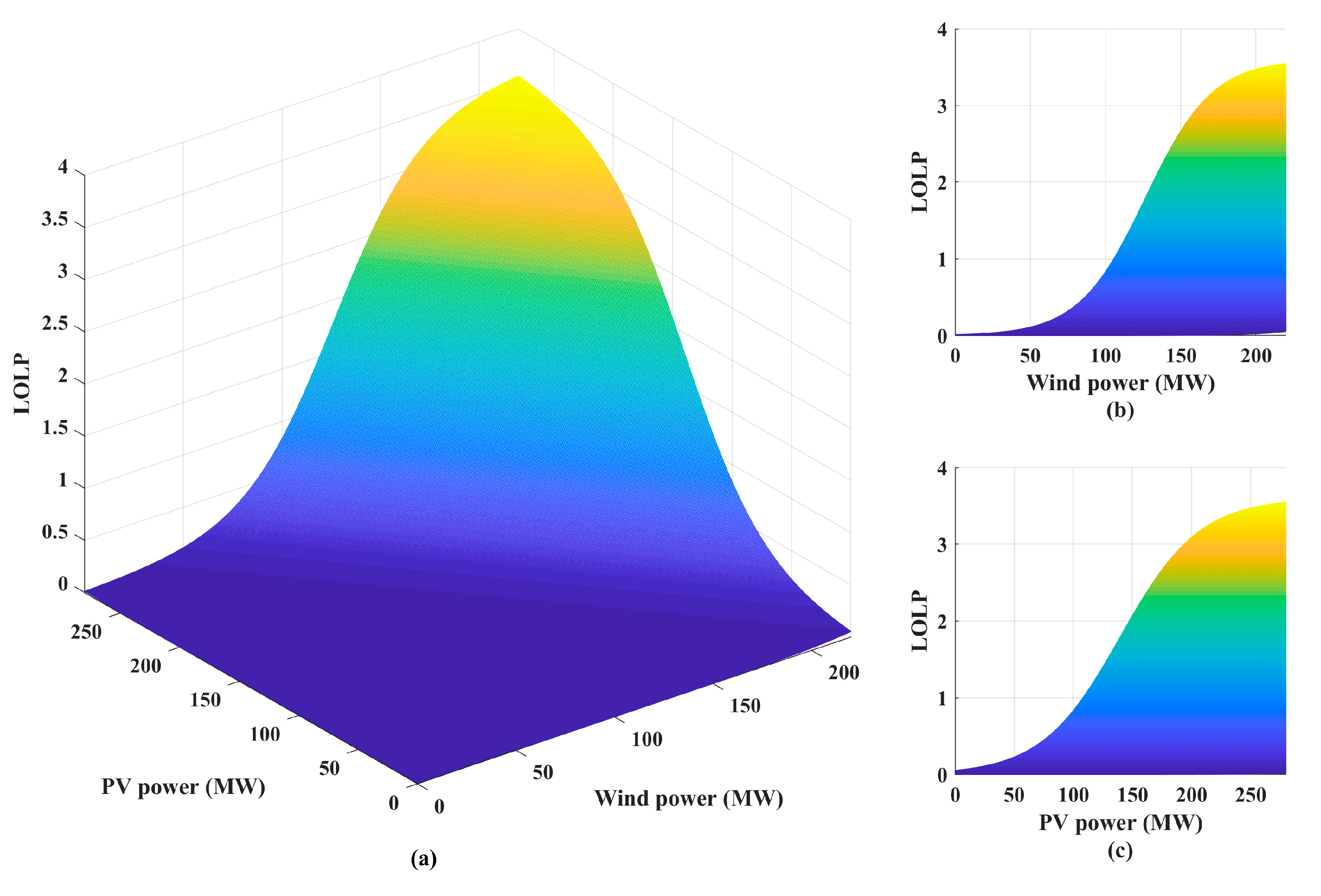
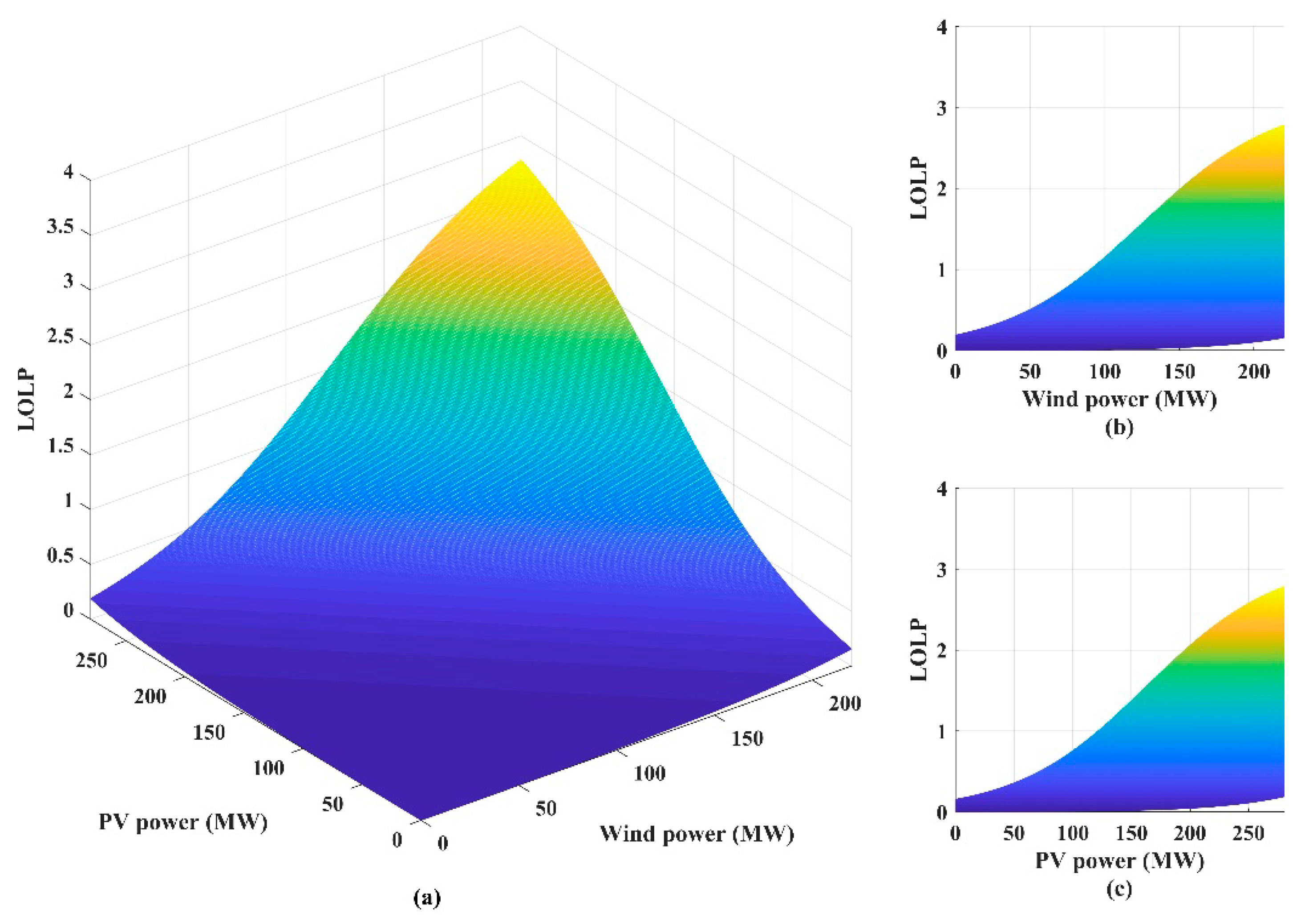
5.1. Reliability Evaluation

The system reliability represented by indices LOLP respect to different installed capacities of wind power and PV power are presented in Figure 5a. In addition, the LOLP variations corresponding to individual renewable generation resources are shown in Figure 5b and Figure 5c, respectively. Figure 5b,c were obtained by projecting the curved surface in Figure 5a onto the “wind power-LOLP” space and “PV power-LOLP” space respectively. It should be noted that the total installed generation capacity was regarded as a constant. Consequently, as the installed capacity of the renewable farms increased, the capacity of traditional generators decreased accordingly. Based on the proportional allocation rule of capacity, the decreased generation amount was shared by all traditional generators. Clearly, the LOLP increased with the growth of the installed capacities of wind power and PV power. Via consideration of this figure, we can obtain the optimal installed renewable generation capacity respect to the acceptable reliability level in power system operation.

To indicate the effect of considering the correlation of wind and PV power, we also evaluated the system reliability without taking into account the correlation of wind and PV power for comparison’s sake. The evaluation result is presented in Figure 6. It can be seen that with the same installed capacities of wind and PV power, LOLP is smaller compared to that considering correlation. This result indicates that the correlation of wind and PV power has an impact on the reliability result, the ignoring of which leads to a relatively optimistic estimate for the system reliability and therefore more load curtailment in the actual power system operation.

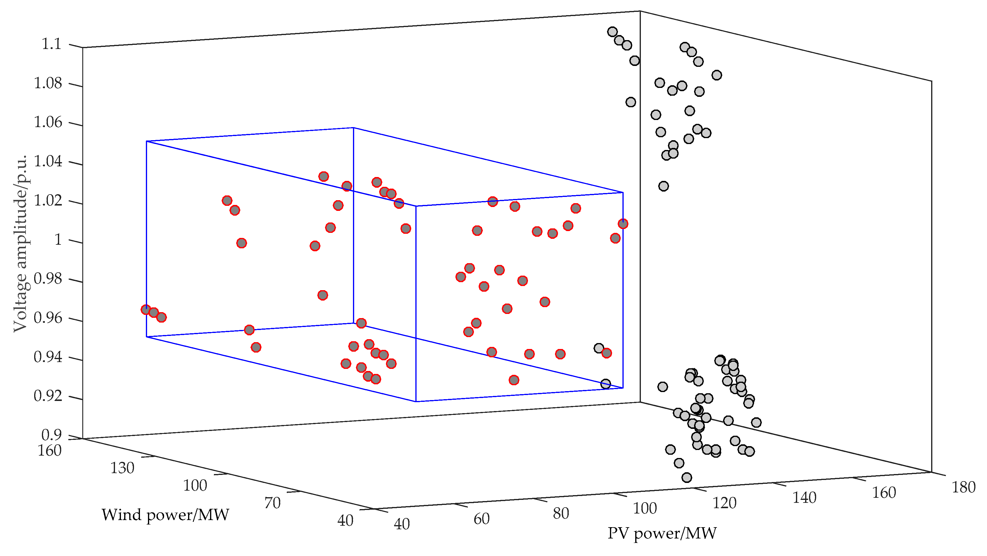
5.2. Voltage Variation

The variation of the system voltage amplitude corresponding to the installed capacities of wind power and PV power is shown in Figure 7. The voltage amplitude with respect to a specific pair of wind and PV power is the voltage of the specific bus whose voltage deviated most from the reference value of 1 in p.u. in all normal scenarios without component failure. In China, the normalized bus voltage amplitude is required to be within 0.95–1.05 in a normal operation state of a power system. As shown in Figure 7, the blue box in three-dimensional space is the acceptable voltage amplitude corresponding to the optimal installed capacities of wind power and PV power. The red circles with a deep gray color are the optimal simulation results. With the proposed model, we can identify the optimal installed capacities of wind power and PV power considering the possible bus voltage variations of the power system.

6. Conclusions

In this study, a novel integration capability evaluation model based on temporal and spatial correlations among different renewable generations have been proposed using a copula model. The aggregation distribution model for wind power generation and PV power generation was formulated based on their temporal and spatial correlations. The integration capacities of wind power and PV power were evaluated based on the reliability analysis of power systems. Two-dimensional evaluation results were produced based on the temporal and spatial model. The optimal integration capacities of wind power and PV power in a power grid can be determined according to the requirements of system reliability. The simulation results demonstrate that the proposed model can give a comprehensive evaluation of the renewable generation integration ability of power systems.

References

1. Council, G.W.E. Global Wind Report 2018; GWEC: Brussels, Belgium, 2018. [Google Scholar]
2. SolarPower Europe. Global Market Outlook For Solar Power 2018–2022; SolarPower Europe: Brussels, Belgium, 2018. [Google Scholar]
3. Lin, Y.; Yang, M.; Wan, C.; Wang, J.; Song, Y. A Multi-model Combination Approach for Probabilistic Wind Power Forecasting. IEEE Trans. Sustain. Energy 2018, 10, 226–237. [Google Scholar] [CrossRef]
4. Wan, C.; Lin, J.; Song, Y.; Xu, Z.; Yang, G. Probabilistic forecasting of photovoltaic generation: An efficient statistical approach. IEEE Trans. Power Syst. 2017, 32, 2471–2472. [Google Scholar] [CrossRef]
5. Yang, X.; Song, Y.; Wang, G.; Wang, W. A comprehensive review on the development of sustainable energy strategy and implementation in China. IEEE Trans. Sustain. Energy 2010, 1, 57–65. [Google Scholar] [CrossRef]
6. Heydt, G.T. The next generation of power distribution systems. IEEE Trans. Smart Grid 2010, 1, 225–235. [Google Scholar] [CrossRef]
7. Lin, Y.; Ding, Y.; Song, Y.; Guo, C. A Multi-State Model for Exploiting the Reserve Capability of Wind Power. IEEE Trans. Power Syst. 2018, 33, 3358–3372. [Google Scholar] [CrossRef]
8. Lund, P.D.; Lindgren, J.; Mikkola, J.; Salpakari, J. Review of energy system flexibility measures to enable high levels of variable renewable electricity. Renew. Sustain. Energy Rev. 2015, 45, 785–807. [Google Scholar] [CrossRef] [Green Version]
9. Eftekharnejad, S.; Vittal, V.; Heydt, G.T.; Keel, B.; Loehr, J. Impact of increased penetration of photovoltaic generation on power systems. IEEE Trans. Power Syst. 2013, 28, 893–901. [Google Scholar] [CrossRef]
10. Shaaban, M.F.; El-Saadany, E. Accommodating high penetrations of PEVs and renewable DG considering uncertainties in distribution systems. IEEE Trans. Power Syst. 2014, 29, 259–270. [Google Scholar] [CrossRef]
11. Divya, K.; Østergaard, J. Battery energy storage technology for power systems—An overview. Electr. Power Syst. Res. 2009, 79, 511–520. [Google Scholar] [CrossRef]
12. Denholm, P.; Hand, M. Grid flexibility and storage required to achieve very high penetration of variable renewable electricity. Energy Policy 2011, 39, 1817–1830. [Google Scholar] [CrossRef]
13. Liu, Y.; Bebic, J.; Kroposki, B.; De Bedout, J.; Ren, W. Distribution system voltage performance analysis for high-penetration PV. In Proceedings of the Energy 2030 Conference, Atlanta, GA, USA, 17–18 November 2008; pp. 1–8. [Google Scholar]
14. Huber, M.; Dimkova, D.; Hamacher, T. Integration of wind and solar power in Europe: Assessment of flexibility requirements. Energy 2014, 69, 236–246. [Google Scholar] [CrossRef] [Green Version]
15. Tahir, S.; Wang, J.; Baloch, M.H.; Kaloi, G.S. Digital control techniques based on voltage source inverters in renewable energy applications: A Review. Electronics 2018, 7, 18. [Google Scholar] [CrossRef]
16. Connolly, D.; Lund, H.; Mathiesen, B.V.; Leahy, M. A review of computer tools for analysing the integration of renewable energy into various energy systems. Appl. Energy 2010, 87, 1059–1082. [Google Scholar] [CrossRef]
17. Widén, J. Correlations between large-scale solar and wind power in a future scenario for Sweden. IEEE Trans. Sustain. Energy 2011, 2, 177–184. [Google Scholar] [CrossRef]
18. Monforti, F.; Huld, T.; Bódis, K.; Vitali, L.; D’isidoro, M.; Lacal-Arántegui, R. Assessing complementarity of wind and solar resources for energy production in Italy. A Monte Carlo approach. Renew. Energy 2014, 63, 576–586. [Google Scholar] [CrossRef]
19. Chatfield, C. The Analysis of Time Series: An Introduction; CRC Press: Boca Raton, FL, USA, 2016. [Google Scholar]
20. Zhang, Y.; Wang, J.; Wang, X. Review on probabilistic forecasting of wind power generation. Renew. Sustain. Energ. Rev. 2014, 32, 255–270. [Google Scholar] [CrossRef]
21. Bessa, R.J.; Miranda, V.; Botterud, A.; Zhou, Z.; Wang, J. Time-adaptive quantile-copula for wind power probabilistic forecasting. Renew. Energy 2012, 40, 29–39. [Google Scholar] [CrossRef]
22. Sklar, M. Fonctions de repartition an dimensions et leurs marges. Publ. Inst. Statist. Univ. Paris 1959, 8, 229–231. [Google Scholar]
23. Nelsen, R.B. An Introduction to Copulas; Springer Science & Business Media: New York, NY, USA, 2007. [Google Scholar]
24. Angus, J.E. The probability integral transform and related results. SIAM Rev. 1994, 36, 652–654. [Google Scholar] [CrossRef]
25. Li, D.X. On default correlation: A copula function approach. J. Fixed Income 2000. [Google Scholar] [CrossRef]
26. Subcommittee, P.M. IEEE reliability test system. IEEE Trans. Power App. Syst. 1979, 98, 2047–2054. [Google Scholar] [CrossRef]
Figure 1. Photovoltaic (PV) power and wind power time series.
Energies 12 00171 g001
Figure 2. The Auto-Correlation Function (ACF) of PV power generation and wind power generation and Cross-Correlation Function (CCF) values between the series of PV farms and wind farms.
Energies 12 00171 g002
Figure 3. The ACF of PV power generation and wind power generation and CCF values between the series of PV farms and wind farms without zero PV output time.
Energies 12 00171 g003
Figure 4. Scatter plot results of the dependence relationship between the random variables. (a) Scatter plot between the forecast errors of wind power and PV power. (b) Scatter plot between the transformed forecast errors of wind power and PV power.
Energies 12 00171 g004
Figure 5. Loss of load probability (LOLP) variation with respect to installed capacities of wind power and PV power, considering correlations. (a) LOLP with respect to wind power and PV power; (b) LOLP with respect to wind power; (c) LOLP with respect to PV power.
Energies 12 00171 g005
Figure 6. LOLP variation with respect to installed capacities of wind power and PV power, without considering correlations. (a) LOLP with respect to wind power and PV power; (b) LOLP with respect to wind power; (c) LOLP with respect to PV power.
Energies 12 00171 g006
Figure 7. Voltage amplitude variations corresponding to the varying installed capacities of wind power and PV power.
Energies 12 00171 g007