Current Control of a Six-Phase Induction Machine Drive Based on Discrete-Time Sliding Mode with Time Delay Estimation

Abstract

This paper proposes a robust nonlinear current controller that deals with the problem of the stator current control of a six-phase induction motor drive. The current control is performed by using a state-space representation of the system, explicitly considering the unmeasurable states, uncertainties and external disturbances. To estimate these latter effectively, a time delay estimation technique is used. The proposed control architecture consists of inner and outer loops. The inner current control loop is based on a robust discrete-time sliding mode controller combined with a time delay estimation method. As said before, the objective of the time delay estimation is to reconstruct the unmeasurable states and uncertainties, while the sliding mode aims is to suppress the estimation error, to ensure robustness and finite-time convergence of the stator currents to their desired references. The outer loop is based on a proportional-integral controller to control the speed. The stability of the current closed-loop system is proven by establishing sufficient conditions on the switching gains. Experimental work has been conducted to verify the performance and the effectiveness of the proposed robust control scheme for a six-phase induction motor drive. The results obtained have shown that the proposed method allows good performances in terms of current tracking, in their corresponding planes.

1. Introduction

Multiphase drives have received significant interest from the power electronics, control, machines and drives communities due to their good features in comparison with traditional three-phase drives. The features include lower torque ripple, lower current/power per phase and fault-tolerant capabilities without adding extra hardware [1,2,3]. Currently, multiphase drives are extensively used in several applications where high power is required such as ships, wind energy generation systems and electric vehicles [3,4]. In the literature, most of the developed and published control techniques for multiphase Induction Machine (IM) drives are an extension of the ones designed for the three-phase machines such as Proportional-Resonant (PR) [5], Proportional-Integral (PI) Pulse-Width Modulation (PWM) [6], Direct Torque Control (DTC) [7], Predictive Torque Control (PTC) [8], sensorless [9,10] and Model Predictive Control (MPC) [11,12], among others. Recently, the above-mentioned controllers have been extended for multiphase machines under fault situations [13,14,15,16]. However, few published papers have considered robust nonlinear controllers and intelligent techniques such as backstepping [17,18], Sliding Mode Control (SMC) [19,20,21], fuzzy logic [22] and others.

Among the above-mentioned nonlinear controllers, SMC is one of the most widely used and has received particular attention from the automation community due to its three highly-valued properties, namely robustness against matched uncertainties, simplicity of design and finite-time convergence [23,24]. This method forces the system states to reach in finite time the user-selected sliding surface (switching surface) even in the presence of the matched uncertainties using discontinuous inputs [24]. To ensure high performances, the switching gains should be chosen as large as possible to reject the effect of the bounded uncertainties. However, this choice causes the major drawback of SMC, well-known under the name of the chattering phenomenon [25,26]. The latter has an unpleasant impact on system actuators. It can lead to deterioration of the controlled system and/or instability. Once this problem has been identified, many works that tried to solve it were published, and among them, we cite the following:

• The substitution of the discontinuous signum function by linear ones [27]. This method is the well-known SMC based on a boundary layer. This proposition allows the reduction of the chattering phenomenon. However, the finite-time convergence feature is no longer guaranteed. The latter is very desirable when critical convergence time is required.
• Observer-based SMC [28,29]. The issue of designing a robust nonlinear controller in this technique is reduced to the issue of designing a robust nonlinear observer. In other words, if the matched uncertainties are not accurately estimated, the performances obtained will not be satisfactory.
• Higher Order Sliding Mode (HOSM) [30,31,32]. The idea consists of making the switching control term act on the control input derivative, which makes the control input fed into the system continuous. This method gives better performances since it allows higher precision and reduces the chattering phenomenon. However, this approach requires some information, as the first time derivative of the selected sliding surface is not always available for measurements, making the implementation difficult.

Recently, an interesting method that consists of combining SMC with the Time Delay Estimation (TDE) method for uncertain nonlinear systems [33,34] has been developed. The proposed method has been successfully tested on a redundant robot manipulator. The basic idea is to estimate the matched uncertainties that are assumed to be Lipschitz using delayed states and input information. Then, the estimated terms are added to the equivalent controller in order to allow a small choice of the switching gains of the discontinuous controller.

Nevertheless, real-time implementation is generally performed through discrete systems [35]. For this reason, the development of the controller should be done in discrete-time. Consequently, it is suitable for use with a discrete-time model of the six-phase IM during the design procedure since after discretization, the inherent properties of the sliding mode approach can no longer be maintained.

In summary, the aim of this paper is to develop a robust Discrete-time SMC (DSMC) combined with the TDE method for the inner current control loop of an Indirect Rotor Field-Oriented Control (IRFOC) of a six-phase IM drive. The developed controller works for all multiphase machines in several applications as more electric aircraft, ship propulsion, battery-powered electric vehicles, electric traction and hybrid electric vehicles. Experimental validation is presented to show the effectiveness of the current controller in transient and steady-state conditions. The rest of the paper is organized as follows. The mathematical discrete-time model of the considered system is presented in Section 2, while the proposed controller design and detailed stability analysis are explained in Section 3. Experimental results are presented in Section 4. Finally, Section 5 draws some conclusions.

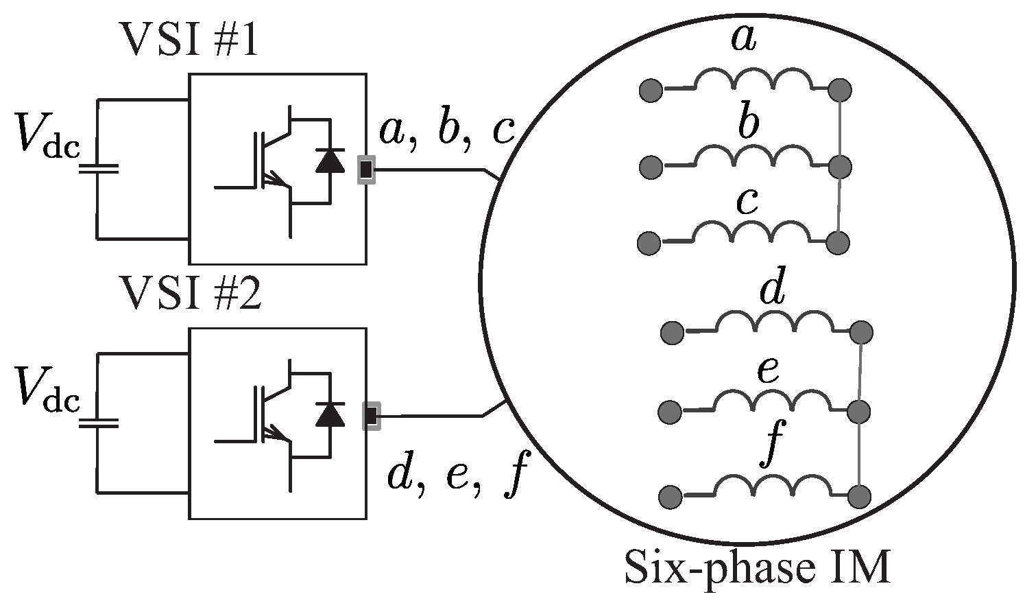
2. Six-Phase IM and VSI Model

The considered system shown in Figure 1 consists of the asymmetrical six-phase IM fed by two two-Level (2L) Voltage Source Inverter (VSI). After using the Vector Space Decomposition (VSD) approach, the decoupling transformation $\mathbf{T}$ gives the $\alpha -\beta$ subspace, which is related to the flux/torque producing components and the loss-producing $x-y$ subspace and a zero-sequence subspace. Then, by using an amplitude-invariant transformation matrix, $\mathbf{T}$ is defined as follows:

$$\mathbf{T}=\frac{1}{3}\left[\begin{array}{cccccc}1& \frac{\sqrt{3}}{2}& -\frac{1}{2}& -\frac{\sqrt{3}}{2}& -\frac{1}{2}& 0\\ 0& \frac{1}{2}& \frac{\sqrt{3}}{2}& \frac{1}{2}& -\frac{\sqrt{3}}{2}& -1\\ 1& -\frac{\sqrt{3}}{2}& -\frac{1}{2}& \frac{\sqrt{3}}{2}& -\frac{1}{2}& 0\\ 0& \frac{1}{2}& -\frac{\sqrt{3}}{2}& \frac{1}{2}& \frac{\sqrt{3}}{2}& -1\\ 1& 0& 1& 0& 1& 0\\ 0& 1& 0& 1& 0& 1\end{array}\right].$$

(1)

The discrete-time model of the system in state-space representation is represented by the following equations [36]:

$$\begin{array}{ccc}\hfill \mathbf{X}(k+1)& =& \mathbf{A}\mathbf{X}\left(k\right)+\mathbf{B}\mathbf{u}\left(k\right)+\mathbf{n}\left(k\right)\hfill \end{array}$$

(2)

$$\begin{array}{ccc}\hfill \mathbf{Y}\left(k\right)& =& \mathbf{C}\mathbf{X}\left(k\right)\hfill \end{array}$$

(3)

In the equations above, the stator and rotor currents are the state vector:

$$\mathbf{X}\left(k\right)={\left[i_{s\alpha }\left(k\right),i_{s\beta }\left(k\right),i_{sx}\left(k\right),i_{sy}\left(k\right),i_{r\alpha }\left(k\right),i_{r\beta }\left(k\right)\right]}^T$$

(4)

while the stator voltages represent the input vector:

$$\mathbf{u}\left(k\right)={\left[u_{s\alpha }\left(k\right),u_{s\beta }\left(k\right),u_{sx}\left(k\right),u_{sy}\left(k\right)\right]}^T$$

(5)

and the stator currents the output vector:

$$\mathbf{Y}\left(k\right)={\left[i_{s\alpha }\left(k\right),i_{s\beta }\left(k\right),i_{sx}\left(k\right),i_{sy}\left(k\right)\right]}^T$$

(6)

and $\mathbf{n}\left(k\right)$ is the $(6\times 1)$ uncertain vector. The stator voltages have a discrete nature due to the VSI model, and the relationship between them is represented as:

$$V_{\mathrm{dc}}\mathbf{T}\mathbf{M}={\left[u_{s\alpha }\left(k\right),u_{s\beta }\left(k\right),u_{sx}\left(k\right),u_{sy}\left(k\right)\right]}^T$$

(7)

where $V_{\mathrm{dc}}$ is the DC-bus voltage, and the VSI model is:

$$\mathbf{M}=\frac{1}{3}\left[\begin{array}{cccccc}2& 0& -1& 0& -1& 0\\ 0& 2& 0& -1& 0& -1\\ -1& 0& 2& 0& -1& 0\\ 0& -1& 0& 2& 0& -1\\ -1& 0& -1& 0& 2& 0\\ 0& -1& 0& -1& 0& 2\end{array}\right]{\mathbf{S}}^T$$

(8)

where $\mathbf{S}=\left[S_a,S_b,S_c,S_d,S_e,S_f\right]$ is the vector of the gating signals with $S_i\in \{0,1\}$. Moreover, the matrices $\mathbf{A}\in R^{6\times 6}$, $\mathbf{B}\in R^{6\times 4}$ and $\mathbf{C}\in R^{4\times 6}$ are defined by:

$$\mathbf{A}=\left[\begin{array}{cccccc}{a}_{11}& a_{12}& 0& 0& a_{15}& a_{16}\\ a_{21}& a_{22}& 0& 0& a_{25}& a_{26}\\ 0& 0& a_{33}& 0& 0& 0\\ 0& 0& 0& a_{44}& 0& 0\\ a_{51}& a_{52}& 0& 0& a_{55}& a_{56}\\ a_{61}& a_{62}& 0& 0& a_{65}& a_{66}\end{array}\right]$$

(9)

$$\mathbf{B}=\left[\begin{array}{cccc}{b}_1& 0& 0& 0\\ 0& b_1& 0& 0\\ 0& 0& b_2& 0\\ 0& 0& 0& b_2\\ b_3& 0& 0& 0\\ 0& b_3& 0& 0\end{array}\right]$$

(10)

$$\mathbf{C}=\left[\begin{array}{cccccc}1& 0& 0& 0& 0& 0\\ 0& 1& 0& 0& 0& 0\\ 0& 0& 1& 0& 0& 0\\ 0& 0& 0& 1& 0& 0\end{array}\right]$$

(11)

where:

$$\begin{array}{ccc}{a}_{11}=a_{22}=1-T_s{c}_2{R}_s\hfill & a_{12}=-a_{21}=T_s{c}_4{L}_m{\omega }_{r\left(k\right)}\hfill & a_{15}=a_{26}=T_s{c}_4{R}_r\hfill \\ a_{16}=-a_{25}=T_s{c}_4{L}_r{\omega }_{r\left(k\right)}\hfill & a_{33}=a_{44}=1-T_s{c}_3{R}_s\hfill & a_{51}=a_{62}=T_s{c}_4{R}_s\hfill \\ a_{52}=-a_{61}=-T_s{c}_5{L}_m{\omega }_{r\left(k\right)}\hfill & a_{55}=a_{66}=1-T_s{c}_5{R}_r\hfill & a_{56}=-a_{65}=-c_5{\omega }_{r\left(k\right)}{T}_s{L}_r\hfill \\ b_1=T_s{c}_2\hfill & b_2=T_s{c}_3\hfill & b_3=-T_s{c}_4\hfill \end{array}$$

with $T_s$ the sampling time and $c_1$ to $c_5$ are defined as: $c_1=L_s{L}_r-L_m^2$, $c_2=\frac{L_r}{c_1}$, $c_3=\frac{1}{L_{ls}}$, $c_4=\frac{L_m}{c_1}$, $c_5=\frac{L_s}{c_1}$. The electrical parameters of the systems are $R_s$, $R_r$, $L_r=L_{lr}+L_m$, $L_s=L_{ls}+L_m$, $L_r$ and $L_m$. The rotor electrical speed ${\omega }_r$ is related to the load torque $T_l$ and the generated torque $T_e$ as follows:

$$J_m{\dot{\omega }}_r+B_m{\omega }_r=P\left(T_e-T_l\right)$$

(12)

$${\omega }_r=P{\omega }_m$$

(13)

where $J_m$ denotes the inertia coefficient, $B_m$ denotes the friction coefficient, P denotes the number of pole pairs and the generated torque $T_e$ is defined by:

$$T_e=3P\left({\psi }_{s\alpha }{i}_{s\beta }-{\psi }_{s\beta }{i}_{s\alpha }\right)$$

(14)

where ${\psi }_{s\alpha }$ and ${\psi }_{s\beta }$ are the stator fluxes.

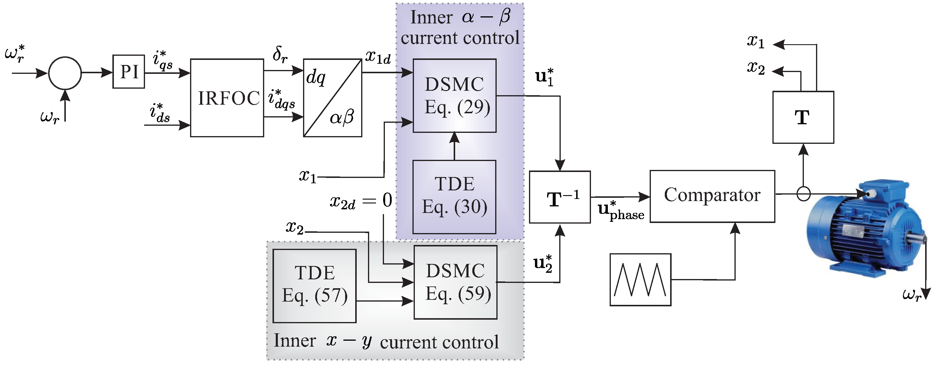
3. Controller Design and Stability Analysis

3.1. Outer Speed Control Loop

A two-degree PI controller with a saturation stage, introduced in [37], is used as the outer speed control loop, based on the IRFOC method. In this loop, the output of the PI regulator is used to get the dynamic current reference $i_{sq}^{*}\left(k\right)$. In addition, the slip frequency ${\omega }_{sl}\left(k\right)$ calculation is obtained from the current references $i_{sd}^{*}\left(k\right),i_{sq}^{*}\left(k\right)$ in the dynamic reference frame and the electrical parameters of the six-phase IM, as shown in Figure 2.

3.2. Inner Current Control Loop

The inner loop aims to control the stator currents. For this purpose, the DSMC with TDE method will be derived to ensure the finite-time convergence of the stator currents in the $\alpha -\beta$ and the $x-y$ planes to their desired references with high accuracy even if some states are not measurable (i.e., rotor currents) and in the presence of uncertainties. First of all, let us decompose the discrete system described in (2) into three sub-systems as follows:

$$\begin{array}{ccc}\hfill {\mathbf{x}}_1(k+1)& =& {\mathbf{A}}_1{\mathbf{x}}_1\left(k\right)+{\overline{\mathbf{A}}}_1{\mathbf{x}}_3\left(k\right)+{\mathbf{B}}_1{\mathbf{u}}_1\left(k\right)+{\eta }_1\left(k\right)\hfill \end{array}$$

(15)

$$\begin{array}{ccc}\hfill {\mathbf{x}}_2(k+1)& =& {\mathbf{A}}_2{\mathbf{x}}_2\left(k\right)+{\mathbf{B}}_2{\mathbf{u}}_2\left(k\right)+{\eta }_2\left(k\right)\hfill \end{array}$$

(16)

$$\begin{array}{ccc}\hfill {\mathbf{x}}_3(k+1)& =& {\mathbf{A}}_3{\mathbf{x}}_1\left(k\right)+{\overline{\mathbf{A}}}_3{\mathbf{x}}_3\left(k\right)+{\mathbf{B}}_3{\mathbf{u}}_1\left(k\right)+{\eta }_3\left(k\right)\hfill \end{array}$$

(17)

where the stator and rotor current state vectors:

$$\begin{array}{ccc}\hfill {\mathbf{x}}_1\left(k\right)& =& {\left[i_{s\alpha }\left(k\right),i_{s\beta }\left(k\right)\right]}^T\hfill \end{array}$$

(18)

$$\begin{array}{ccc}\hfill {\mathbf{x}}_2\left(k\right)& =& {\left[i_{sx}\left(k\right),i_{sy}\left(k\right)\right]}^T\hfill \end{array}$$

(19)

$$\begin{array}{ccc}\hfill {\mathbf{x}}_3\left(k\right)& =& {\left[i_{r\alpha }\left(k\right),i_{r\beta }\left(k\right)\right]}^T\hfill \end{array}$$

(20)

while the stator voltages represent the input vectors:

$$\begin{array}{ccc}\hfill {\mathbf{u}}_1\left(k\right)& =& {\left[u_{s\alpha }\left(k\right),u_{s\beta }\left(k\right)\right]}^T\hfill \end{array}$$

(21)

$$\begin{array}{ccc}\hfill {\mathbf{u}}_2\left(k\right)& =& {\left[u_{sx}\left(k\right),u_{sy}\left(k\right)\right]}^T\hfill \end{array}$$

(22)

and ${\eta }_1\left(k\right)={\left[n_1\left(k\right),n_2\left(k\right)\right]}^T$, ${\eta }_2\left(k\right)={\left[n_3\left(k\right),n_4\left(k\right)\right]}^T$ and ${\eta }_3\left(k\right)={\left[n_5\left(k\right),n_6\left(k\right)\right]}^T$ denote the uncertain vectors. The matrices ${\mathbf{A}}_1$, ${\overline{\mathbf{A}}}_1$, ${\mathbf{A}}_2$, ${\mathbf{A}}_3$, ${\overline{\mathbf{A}}}_3$, ${\mathbf{B}}_1$, ${\mathbf{B}}_2$ and ${\mathbf{B}}_3$ are defined as follows:

$${\mathbf{A}}_1=\left[\begin{array}{cc}{a}_{11}& a_{12}\\ a_{21}& a_{22}\end{array}\right],{\mathbf{A}}_2=\left[\begin{array}{cc}{a}_{33}& 0\\ 0& a_{44}\end{array}\right],{\mathbf{A}}_3=\left[\begin{array}{cc}{a}_{51}& a_{52}\\ a_{61}& a_{62}\end{array}\right],{\overline{\mathbf{A}}}_1=\left[\begin{array}{cc}{a}_{15}& a_{16}\\ a_{25}& a_{26}\end{array}\right]$$

$${\overline{\mathbf{A}}}_3=\left[\begin{array}{cc}{a}_{55}& a_{56}\\ a_{65}& a_{66}\end{array}\right],{\mathbf{B}}_1=\left[\begin{array}{cc}{b}_1& 0\\ 0& b_1\end{array}\right],{\mathbf{B}}_2=\left[\begin{array}{cc}{b}_2& 0\\ 0& b_2\end{array}\right],{\mathbf{B}}_3=\left[\begin{array}{cc}{b}_3& 0\\ 0& b_3\end{array}\right]$$

3.2.1. Control of Stator Current in the $\alpha -\beta$ Sub-Space

To achieve our control objective, let ${\mathbf{x}}_1^{*}\left(k\right)=i_{s\varphi }^{*}\left(k\right)={\left[i_{s\alpha }^{*}\left(k\right),i_{s\beta }^{*}\left(k\right)\right]}^T$ be the vector of desired references with $\varphi \in \{\alpha ,\beta \}$ and ${\mathbf{e}}_{\varphi }\left(k\right)={\mathbf{x}}_1\left(k\right)-{\mathbf{x}}_1^{*}\left(k\right)=i_{s\varphi }\left(k\right)-i_{s\varphi }^{*}\left(k\right)$ be the vector of tracking error. As the relative degree of the stator current in $\alpha -\beta$ sub-space is equal to one, then, the sliding surface [24] is selected to be the error variable as follows:

$$\sigma \left(k\right)={\mathbf{e}}_{\varphi }\left(k\right)$$

(23)

In the DSMC design, the following conditions must be satisfied to achieve an ideal sliding motion:

$$\sigma \left(k\right)=0,\sigma (k+1)=0$$

(24)

where $\sigma (k+1)$ is computed as:

$$\begin{array}{cc}\hfill \sigma (k+1)& ={\mathbf{e}}_{\varphi }(k+1)={\mathbf{x}}_1(k+1)-{\mathbf{x}}_1^{*}(k+1)\hfill \\ & ={\mathbf{A}}_1{\mathbf{x}}_1\left(k\right)+{\overline{\mathbf{A}}}_1{\mathbf{x}}_3\left(k\right)+{\mathbf{B}}_1{\mathbf{u}}_1\left(k\right)+{\eta }_1\left(k\right)-{\mathbf{x}}_1^{*}(k+1)\hfill \end{array}$$

(25)

The control obtained by setting $\sigma (k+1)=0$ does not ensure robustness and finite-time convergence. For these reasons, the following reaching law is selected:

$$\sigma (k+1)=\mathsf{\Lambda }\sigma \left(k\right)-T_s\rho \mathrm{sign}\left(\sigma \left(k\right)\right)$$

(26)

where $\mathsf{\Lambda }=\mathrm{diag}({\lambda }_1,{\lambda }_2)$ with $0<{\lambda }_i<1$ for $i=1,2$, $\rho \in R^{2\times 2}$ is a diagonal positive matrix and $\mathrm{sign}\left(\sigma \left(k\right)\right)={\left[\mathrm{sign}\left({\sigma }_1\left(k\right)\right),\mathrm{sign}\left({\sigma }_2\left(k\right)\right)\right]}^T$ with:

$$\mathrm{sign}\left({\sigma }_i\left(k\right)\right)=\left\{\begin{array}{cc}1,& \mathrm{if}{\sigma }_i\left(k\right)>0\\ 0,& \mathrm{if}{\sigma }_i\left(k\right)=0\\ -1,& \mathrm{if}{\sigma }_i\left(k\right)<0\end{array}\right.$$

(27)

Then, using (25) and (26), the DSMC law for the stator current in the $\alpha -\beta$ sub-space is obtained as:

$${\mathbf{u}}_1\left(k\right)=-{\mathbf{B}}_1^{-1}\left[{\mathbf{A}}_1{\mathbf{x}}_1\left(k\right)+{\overline{\mathbf{A}}}_1{\mathbf{x}}_3\left(k\right)+{\eta }_1\left(k\right)-{\mathbf{x}}_1^{*}(k+1)-\mathsf{\Lambda }\sigma \left(k\right)+T_s\rho \mathrm{sign}\left(\sigma \left(k\right)\right)\right]$$

(28)

The control performance might not be satisfactory since the above equation is in terms of the rotor currents ${\mathbf{x}}_3\left(k\right)$ that are not measurable and the uncertain vector ${\eta }_1\left(k\right)$. Assuming that ${\mathbf{x}}_3\left(k\right)$ and ${\eta }_1\left(k\right)$ do not fluctuate widely between two consecutive sampling times, the TDE method [31,38] can be used to obtain an approximation as:

$$\begin{array}{cc}\hfill {\overline{\mathbf{A}}}_1{\widehat{\mathbf{x}}}_3\left(k\right)+{\widehat{\eta }}_1\left(k\right)& \cong {\overline{\mathbf{A}}}_1{\mathbf{x}}_3(k-1)+{\eta }_1(k-1)\hfill \\ \hfill & ={\mathbf{x}}_1\left(k\right)-{\mathbf{A}}_1{\mathbf{x}}_1(k-1)-{\mathbf{B}}_1{\mathbf{u}}_1(k-1)\hfill \end{array}$$

(29)

Definition 1.

For a discrete-time system, a quasi-sliding mode is said to be a trajectory in the vicinity of the sliding surface, such that $|\sigma (k)|<\epsilon$ and where $\epsilon >0$ is the quasi-sliding mode bandwidth. In order to ensure a convergent quasi-sliding mode, the conditions given in [31,39] that are necessary and sufficient must be verified for each sliding surface, i.e.:

$$\begin{array}{c}\hfill \left\{\begin{array}{cc}{\sigma }_i\left(k\right)>\epsilon \hfill & \Rightarrow -\epsilon \le {\sigma }_i(k+1)<{\sigma }_i\left(k\right)\hfill \\ {\sigma }_i\left(k\right)<-\epsilon \hfill & \Rightarrow {\sigma }_i\left(k\right)<{\sigma }_i(k+1)\le \epsilon \hfill \\ |{\sigma }_i\left(k\right)|\le \epsilon \hfill & \Rightarrow |{\sigma }_i(k+1)|\le \epsilon \hfill \end{array}\right.\end{array}$$

(30)

Theorem 1.

If the following condition is satisfied for i= 1, 2:

$${\rho }_i>\frac{1}{T_s}{\delta }_i,$$

(31)

then, the DSMC with TDE method for the stator currents in the $\alpha -\beta$ sub-space (15) given by:

$${\mathbf{u}}_1\left(k\right)=-{\mathbf{B}}_1^{-1}\left[{\mathbf{A}}_1{\mathbf{x}}_1\left(k\right)+{\overline{\mathbf{A}}}_1{\widehat{\mathbf{x}}}_3\left(k\right)+{\widehat{\eta }}_1\left(k\right)-{\mathbf{x}}_1^{*}(k+1)-\mathsf{\Lambda }\sigma \left(k\right)-T_s\rho \mathrm{sign}\left(\sigma \left(k\right)\right)\right]$$

(32)

ensures a quasi sliding mode. Moreover, each system trajectory will reach its corresponding sliding surface (23) within at most k${}_i^{{}^{\prime }}$ + 1 steps, where for i= 1, 2:

$$k_i^{{}^{\prime }}={\displaystyle \frac{|{\sigma }_i\left(0\right)|}{T_s{\rho }_i-{\delta }_i}}$$

(33)

Proof of Theorem 1.

Substituting the obtained discrete time controller (32) into Equation (25) leads to:

$$\sigma (k+1)=\mathsf{\Lambda }\sigma \left(k\right)+\mathbf{E}\left(k\right)-T_s\rho \mathrm{sign}\left(\sigma \left(k\right)\right)$$

(34)

where $\mathbf{E}\left(k\right)={\overline{\mathbf{A}}}_1\left(x_3\left(k\right)-{\widehat{x}}_3\left(k\right)\right)+\left({\eta }_1\left(k\right)-{\widehat{\eta }}_1\left(k\right)\right)$ is the bounded TDE error such as for $i=1,2$:

$$|E_i\left(k\right)|<{\delta }_i$$

(35)

Now, choose $\epsilon =T_s{\rho }_i+{\delta }_i$. Hence, Equation (30) can be rewritten as:

$$\begin{array}{c}{\sigma }_i\left(k\right)>T_s{\rho }_i+{\delta }_i\Rightarrow -T_s{\rho }_i-{\delta }_i\le {\sigma }_i(k+1)<{\sigma }_i\left(k\right)\hfill \\ {\sigma }_i\left(k\right)<-T_s{\rho }_i-{\delta }_i\Rightarrow {\sigma }_i\left(k\right)<{\sigma }_i(k+1)\le T_s{\rho }_i+{\delta }_i\hfill \\ |{\sigma }_i\left(k\right)|\le T_s{\rho }_i+{\delta }_i\Rightarrow |{\sigma }_i(k+1)|\le T_s{\rho }_i+{\delta }_i.\hfill \end{array}$$

(36)

• Consider the first case where ${\sigma }_i\left(k\right)>T_s{\rho }_i+{\delta }_i$, then ${\sigma }_i\left(k\right)>0$, $\mathrm{sign}\left({\sigma }_i\left(k\right)\right)=1$ and:

  $$\begin{array}{c}{\sigma }_i(k+1)={\lambda }_i{\sigma }_i\left(k\right)+E_i\left(k\right)-T_s{\rho }_i\hfill \\ {\sigma }_i(k+1)-{\sigma }_i\left(k\right)=E_i\left(k\right)+({\lambda }_i-1){\sigma }_i\left(k\right)-T_s{\rho }_i.\hfill \end{array}$$

  (37)
  If the condition in (31) is satisfied, then ${\sigma }_i(k+1)-{\sigma }_i\left(k\right)<0\Rightarrow {\sigma }_i(k+1)<{\sigma }_i\left(k\right)$.
  Moreover, $-T_s{\rho }_i-{\delta }_i\le {\sigma }_i(k+1)$ can be written as:

  $${\lambda }_i{\sigma }_i\left(k\right)+E_i\left(k\right)-T_s{\rho }_i\ge -T_s{\rho }_i-{\delta }_i.$$

  (38)
  Hence:

  $${\sigma }_i\left(k\right)\ge \frac{1}{{\lambda }_i}\left(E_i\left(k\right)-{\delta }_i\right),$$

  (39)

  since ${\sigma }_i\left(k\right)>0$ and $(E_i\left(k\right)-{\delta }_i)<0$, then the above inequality is always true.
• Consider the second case where ${\sigma }_i\left(k\right)<-T_s{\rho }_i-{\delta }_i$. This implies ${\sigma }_i\left(k\right)<0$ and $\mathrm{sign}\left({\sigma }_i\left(k\right)\right)=-1$. Then, let us rewrite ${\sigma }_i\left(k\right)<{\sigma }_i(k+1)$ as follows:

  $$\begin{array}{cc}\hfill {\sigma }_i\left(k\right)& <{\lambda }_i{\sigma }_i\left(k\right)+E_i\left(k\right)+T_s{\rho }_i\hfill \\ \hfill (1-{\lambda }_i){\sigma }_i\left(k\right)& <E_i\left(k\right)+T_s{\rho }_i\hfill \end{array}$$

  (40)

  which is always true since ${\rho }_i>{\displaystyle \frac{1}{T_s}}{\delta }_i$.
  Moreover, ${\sigma }_i(k+1)<T_s{\rho }_i+{\delta }_i$ can be rewritten as:

  $${\lambda }_i{\sigma }_i\left(k\right)+E_i\left(k\right)+T_s{\rho }_i<T_s{\rho }_i+{\delta }_i.$$

  (41)
  Since ${\sigma }_i\left(k\right)<0$ and ${\delta }_i>E_i\left(k\right)$, then, it is obvious that the inequality in (15) is always true.
• Consider the third case where $|{\sigma }_i\left(k\right)|\le \epsilon$, then:
  • if ${\sigma }_i\left(k\right)>0$, then $|{\sigma }_i\left(k\right)|\le \epsilon$ becomes:

    $$0<{\sigma }_i\left(k\right)<\epsilon .$$

    (42)
    Multiplying (42) by ${\lambda }_i$ and adding $E_i\left(k\right)-T_s{\rho }_i$ to all the part leads to:

    $$\begin{array}{cc}\hfill E_i\left(k\right)-T_s{\rho }_i<{\sigma }_i(k+1)& <E_i\left(k\right)-T_s{\rho }_i+{\lambda }_i\epsilon \hfill \\ \hfill -\epsilon <{\sigma }_i(k+1)& <\epsilon \hfill \\ \hfill |{\sigma }_i(k+1)|& \le \epsilon \hfill \end{array}$$

    (43)
  • if ${\sigma }_i\left(k\right)<0$, then $|{\sigma }_i\left(k\right)|\le \epsilon$ becomes:

    $$-\epsilon <{\sigma }_i\left(k\right)<0.$$

    (44)
    Once again, multiplying (44) by ${\lambda }_i$ and adding $E_i\left(k\right)+T_s{\rho }_i$ to all the parts gives:

    $$\begin{array}{cc}\hfill E_i\left(k\right)+T_s{\rho }_i-{\lambda }_i\epsilon <{\sigma }_i(k+1)& <E_i\left(k\right)+T_s{\rho }_i\hfill \\ \hfill -\epsilon <{\sigma }_i(k+1)& <\epsilon \hfill \\ \hfill |{\sigma }_i(k+1)|& \le \epsilon \hfill \end{array}$$

    (45)
  Hence:

  $$|{\sigma }_i(k+1)|<\epsilon =T_s{\rho }_i+{\delta }_i.$$

  (46)

Since the conditions in (36) are met, the existence of a convergent quasi sliding mode has been established. Consequently, the proposed DSMC with TDE method in (32) is stable.

Now, let us demonstrate by contradiction according to (34) that Equation (33) is true. For this part, let us assume that ${\sigma }_i\left(0\right)\ne 0$ and $\mathrm{sign}\left({\sigma }_i\left(0\right)\right)=\mathrm{sign}\left({\sigma }_i\left(1\right)\right)=\cdots =\mathrm{sign}\left({\sigma }_i(k^{{}^{\prime }}+1)\right)$.

• Consider the first case where ${\sigma }_i\left(0\right)>0$ and ${\sigma }_i\left(m\right)>0$ for all $m\le (k_i^{{}^{\prime }}+1)$. Then:

  $$\begin{array}{cc}\hfill {\sigma }_i\left(1\right)& ={\lambda }_i{\sigma }_i\left(0\right)+E_i\left(0\right)-T_s{\rho }_i\hfill \\ & \le {\sigma }_i\left(0\right)+E_i\left(0\right)-T_s{\rho }_i\hfill \\ \hfill {\sigma }_i\left(2\right)& \le {\sigma }_i\left(1\right)+E_i\left(1\right)-T_s{\rho }_i\hfill \\ & \le {\sigma }_i\left(0\right)+E_i\left(0\right)+E_i\left(1\right)-2T_s{\rho }_i\hfill \\ \hfill ⋮\\ \hfill {\sigma }_i\left(m\right)& \le {\sigma }_i(m-1)+E_i(m-1)-T_s{\rho }_i\hfill \\ & \le {\sigma }_i\left(0\right)+\sum _{j=0}^{m-1}{E}_i\left(j\right)-m{T}_s{\rho }_i\hfill \\ & \le |{\sigma }_i\left(0\right)|+m\left[{\delta }_i-T_s{\rho }_i\right].\hfill \end{array}$$

  (47)
  Hence, it is obvious that $k_i^{{}^{\prime }}$ ensures that:

  $$|{\sigma }_i\left(0\right)|+k_i^{{}^{\prime }}\left[{\delta }_i-T_s{\rho }_i\right]=0.$$

  (48)
  It follows that:

  $$\begin{array}{cc}\hfill {\sigma }_i(k_i^{{}^{\prime }}+1)& \le |{\sigma }_i\left(0\right)|+(k_i^{{}^{\prime }}+1)\left[{\delta }_i-T_s{\rho }_i\right]\hfill \\ & <|{\sigma }_i\left(0\right)|+k_i^{{}^{\prime }}\left[{\delta }_i-T_s{\rho }_i\right]=0\hfill \end{array}$$

  (49)

  which is contradictory to the fact that ${\sigma }_i\left(m\right)>0,\forall m\le (k_i^{{}^{\prime }}+1)$.
• Consider the second case where ${\sigma }_i\left(0\right)<0$ and ${\sigma }_i\left(m\right)<0$ for all $m\le (k_i^{{}^{\prime }}+1)$. Then:

  $$\begin{array}{cc}\hfill {\sigma }_i\left(1\right)& ={\lambda }_i{\sigma }_i\left(0\right)+E_i\left(0\right)+T_s{\rho }_i\hfill \\ & \ge {\sigma }_i\left(0\right)+E_i\left(0\right)+T_s{\rho }_i\hfill \\ \hfill {\sigma }_i\left(2\right)& \ge {\sigma }_i\left(1\right)+E_i\left(1\right)+T_s{\rho }_i\hfill \\ & \ge {\sigma }_i\left(0\right)+E_i\left(0\right)+E_i\left(1\right)+2T_s{\rho }_i\hfill \\ \hfill ⋮\\ \hfill {\sigma }_i\left(m\right)& \ge {\sigma }_i(m-1)+E_i(m-1)+T_s{\rho }_i\hfill \\ & \ge {\sigma }_i\left(0\right)+\sum _{j=0}^{m-1}{E}_i\left(j\right)+m{T}_s{\rho }_i\hfill \\ & \ge -|{\sigma }_i\left(0\right)|+m\left[T_s{\rho }_i-{\delta }_i\right]\hfill \end{array}$$

  (50)
  Once again, it is obvious that $k_i^{{}^{\prime }}$ verifies:

  $$-|{\sigma }_i\left(0\right)|+k_i^{{}^{\prime }}\left[T_s{\rho }_i-{\delta }_i\right]=0.$$

  (51)
  It follows that:

  $$\begin{array}{cc}\hfill {\sigma }_i(k_i^{{}^{\prime }}+1)& \ge -|{\sigma }_i\left(0\right)|+(k_i^{{}^{\prime }}+1)\left[T_s{\rho }_i-{\delta }_i\right]\hfill \\ & >-|{\sigma }_i\left(0\right)|+k_i^{{}^{\prime }}\left[T_s{\rho }_i-{\delta }_i\right]=0\hfill \end{array}$$

  (52)

  which is contradictory to the fact that ${\sigma }_i\left(m\right)<0,\forall m\le (k_i^{{}^{\prime }}+1)$.

This concludes the proof of Theorem 1. □

3.2.2. Control of Stator Current in the $x-y$ Sub-Space

In this section, the same methodology used previously for the stator current ${\mathbf{x}}_1\left(k\right)$ will be adopted to control the stator current in the $x-y$ sub-space. In this case, the sliding surface is selected as follows:

$${\sigma }^{″}\left(k\right)={\mathbf{e}}_{s_{xy}}\left(k\right)={\mathbf{x}}_2\left(k\right)-{\mathbf{x}}_2^{*}\left(k\right)$$

(53)

where ${\mathbf{x}}_2^{*}\left(k\right)={[i_{sx}^{*}\left(k\right),i_{sy}^{*}\left(k\right)]}^T$ is the desired $x-y$ current and ${\mathbf{e}}_{s_{xy}}\left(k\right)$ denotes the tracking error variable. Hence, ${\sigma }^{″}(k+1)$ is computed as follows:

$$\begin{array}{cc}\hfill {\sigma }^{″}(k+1)& ={\mathbf{e}}_{s_{xy}}(k+1)={\mathbf{x}}_2(k+1)-{\mathbf{x}}_2^{*}(k+1)\hfill \\ & ={\mathbf{A}}_2{\mathbf{x}}_2\left(k\right)+{\mathbf{B}}_2{\mathbf{u}}_2\left(k\right)+{\eta }_2\left(k\right)-{\mathbf{x}}_2^{*}(k+1).\hfill \end{array}$$

(54)

The discrete-time controller is obtained by solving:

$${\sigma }^{″}(k+1)=\mathsf{\Gamma }{\sigma }^{″}\left(k\right)-T_s\varrho \mathrm{sign}\left({\sigma }^{″}\left(k\right)\right)$$

(55)

where $\mathsf{\Gamma }=\mathrm{diag}({\mathsf{\Gamma }}_1,{\mathsf{\Gamma }}_2)$ with $0<{\mathsf{\Gamma }}_i<1$ for $i=1,2$, $\varrho \in R^{2\times 2}$ is a diagonal positive matrix and $\mathrm{sign}\left({\sigma }^{″}\left(k\right)\right)={\left[\mathrm{sign}\left({\sigma }_1^{″}\left(k\right)\right),\mathrm{sign}\left({\sigma }_2^{″}\left(k\right)\right)\right]}^T$, and by substituting the uncertain vector ${\eta }_2\left(k\right)$ by its estimate using TDE method:

$$\begin{array}{cc}\hfill {\widehat{\eta }}_2\left(k\right)& \cong {\eta }_2(k-1)\hfill \\ & ={\mathbf{x}}_2\left(k\right)-{\mathbf{A}}_2{\mathbf{x}}_2(k-1)-{\mathbf{B}}_2{\mathbf{u}}_2(k-1).\hfill \end{array}$$

(56)

Theorem 2.

If the controller gains are chosen for i = 1, 2 as follows:

$${\varrho }_i>{\displaystyle \frac{1}{T_s}}{\delta }_i^{″}$$

(57)

with ${\delta }_i^{″}>0$ the upper-bound of the TDE error $E^{″}\left(k\right)={\eta }_2\left(k\right)-{\widehat{\eta }}_2\left(k\right)$, then, the following DSMC with TDE method for the stator current in the $x-y$ sub-space (16) ensures a quasi sliding motion:

$${\mathbf{u}}_2\left(k\right)=-{\mathbf{B}}_2^{-1}\left[{\mathbf{A}}_2{\mathbf{x}}_2\left(k\right)+{\widehat{\eta }}_2\left(k\right)-{\mathbf{x}}_2^{*}(k+1)-\mathsf{\Gamma }{\sigma }^{″}\left(k\right)+T_s\varrho \mathrm{sign}\left({\sigma }^{″}\left(k\right)\right)\right].$$

(58)

Proof of Theorem 2.

The stability analysis is similar to the one described for the stator currents in the $\alpha -\beta$ sub-space. □

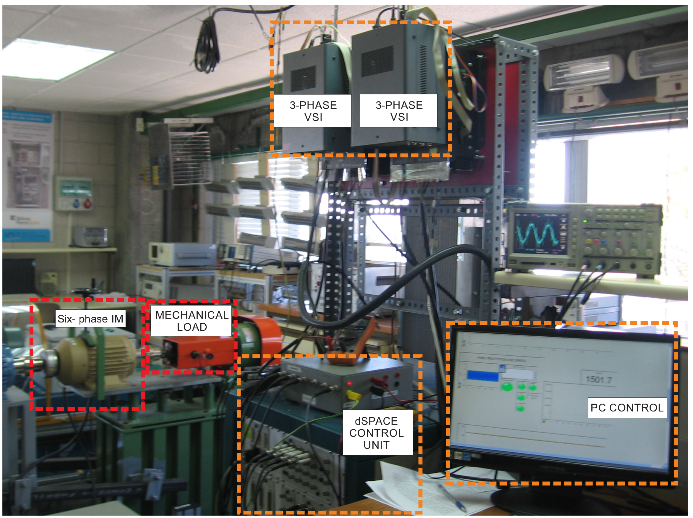
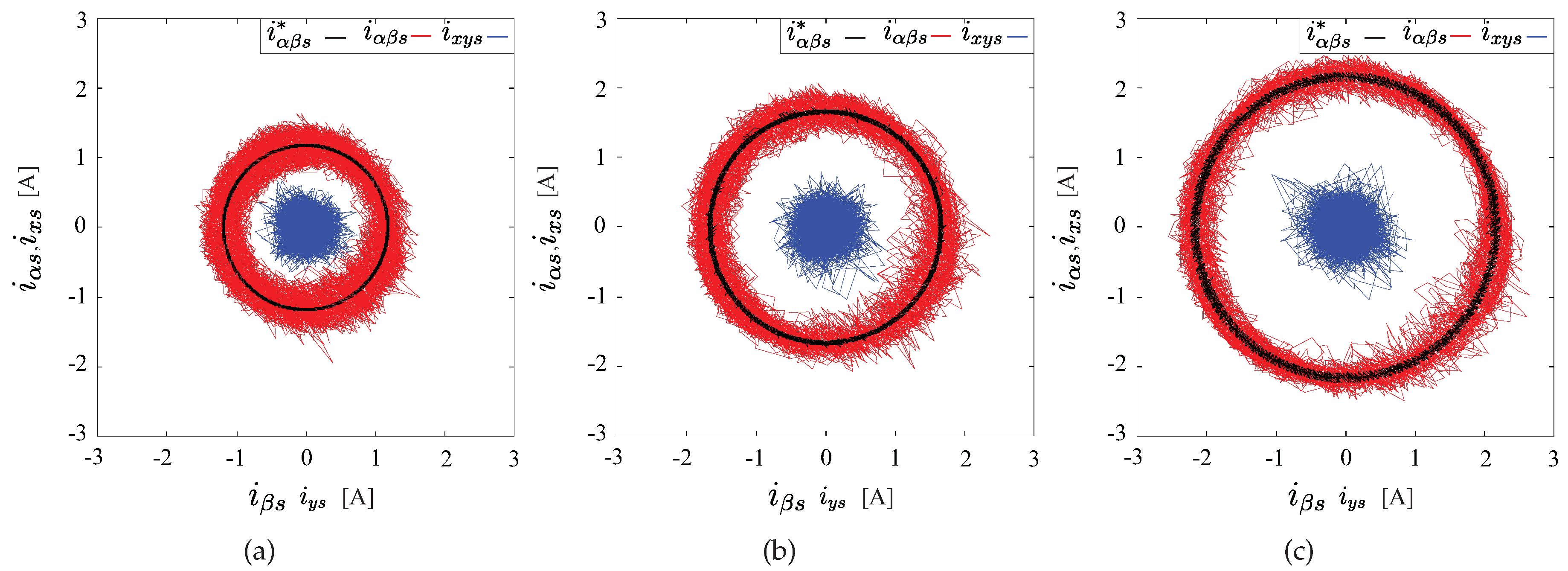
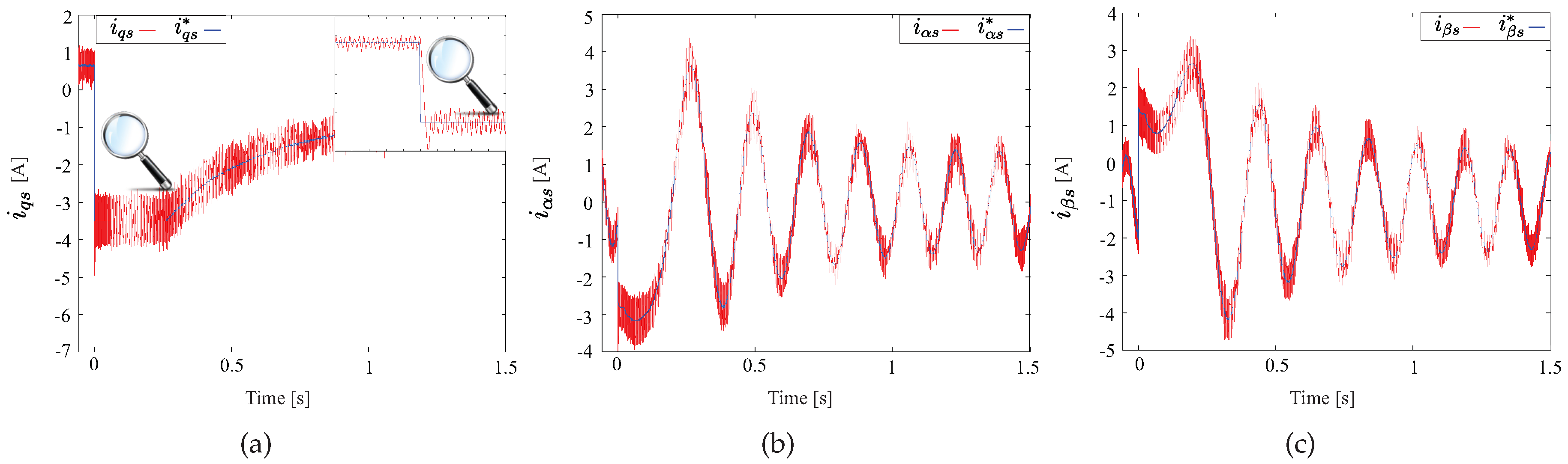
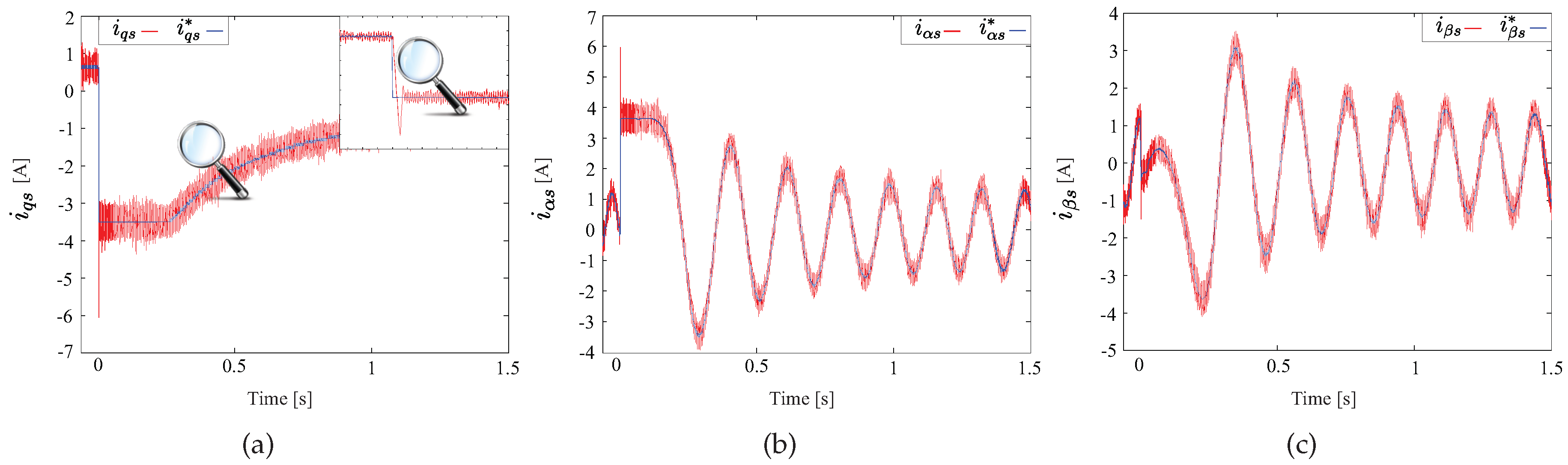
4. Experimental Results

The proposed DSMC technique was tested in order to validate its performance with experimental results obtained in the test bench, and this consisted of a six-phase IM powered by two conventional three-phase VSI, being equivalent to a six-leg VSI, using a constant DC-bus voltage from a DC power supply system. The six-leg VSI was controlled by a dSPACE MABXII DS1401 real-time rapid prototyping platform, with Simulink version 8.2. The results obtained were captured and processed using MATLAB R2013b script. The parameters of the asymmetrical six-phase IM were obtained using conventional methods of the AC time domain and stand-still with VSI supply tests [40,41]. The results are listed in

Table 1. Parameters of the six-phase IM.

Parameter	Value	Parameter	Value	Parameter	Value
$R_r$ ($\mathsf{\Omega }$)	6.9	$L_r$ (mH)	626.8	$P_w$ (kW)	2
$R_s$ ($\mathsf{\Omega }$)	6.7	${\omega }_{m-nom}$ (rpm)	3000	$J_i$ (kg·m${}^2$)	0.07
$L_{ls}$ (mH)	5.3	$L_s$ (mH)	654.4	$B_i$ (kg·m${}^2$/s)	0.0004
$L_m$ (mH)	614	P	1	$V_{\mathrm{dc}}$ (V)	400

. The experimental tests were performed with current sensors LA 55-P s, which had a frequency bandwidth from DC up to 200 kHz. The current measurements were then converted to digital form using a 16-bit A/D converter. The six-phase IM position was obtained with a 1024-ppr incremental encoder, and the rotor speed was estimated from it. Finally, a 5 HP eddy current brake was used to introduce a variable mechanical load on the IM. A block diagram of the experimental bench is shown in Figure 3, including some photos of the equipment.

The performance of the proposed DSMC was analysed in transient and steady-state conditions. The experimental results analysed the controller performance in terms of Mean Squared Error (MSE) between the reference and measured stator currents in the $\alpha -\beta$, $x-y$ and $d-q$ planes. The Root Mean Square (RMS) of the currents in the $d-q$ plane was used to calculate their corresponding Form Factor (FF) and Total Harmonic Distortion (THD) obtained in the $\alpha -\beta$ plane, as well as MSE for rotor speed. The MSE is defined as:

$$\mathrm{MSE}\left(i_{s\mathsf{\Phi }}\right)=\sqrt[]{\frac{1}{N}\sum _{k=1}^N{(i_{s\mathsf{\Phi }}\left(k\right)-i_{s\mathsf{\Phi }}^{*}\left(k\right))}^2}$$

(59)

where N is the number of analysed samples, $i_{s\mathsf{\Phi }}^{*}$ the stator current reference, $i_{s\mathsf{\Phi }}$ the measured stator currents and $\mathsf{\Phi }\in$ $\left\{\alpha ,\beta ,x,y,d,q\right\}$. On the other hand, the THD is calculated as:

$$\mathrm{THD}\left(i_s\right)=\sqrt[]{\frac{1}{i_{s1}^2}\sum _{j=2}^N{\left(i_{sj}\right)}^2}$$

(60)

where $i_{s1}$ is the fundamental stator currents and $i_{sj}$ is the harmonic stator currents. At last, the FF is computed as:

$$\mathrm{FF}\left(i_{dqs}\right)=\frac{i_{dqs-RMS}}{i_{dqs-mean}}.$$

(61)

A fixed d current ($i_{ds}^{*}=1$ A) was used. To perform a mechanical load for the six-phase IM, the eddy current brake was fixed at $1.65$ A. Moreover, the chosen gains of the DSMC with TDE for stator current tracking are:

$$\lambda =\mathrm{diag}(0.5,0.5),{\rho }_1={\rho }_2=100,$$

$$\mathsf{\Gamma }=\mathrm{diag}(0.9,0.9),{\varrho }_1={\varrho }_2=100.$$

The stator current reference in the $x-y$ sub-space was set to zero ($i_{xs}^{*}=i_{ys}^{*}=0$ A) in order to reduce the copper losses. The sampling frequencies used in the tests were 8 kHz and 16 kHz. Three operation points were set for the rotor speed: 500 rpm, 1000 rpm and 1500 rpm for steady-state analysis. For a transient response, a step change in rotor speed was considered from 500 to $-500$ rpm (i.e., a reversal condition).

The proposed technique DSMC was tested under different operating points in steady state and under transient conditions.

Table 2. Performance analysis of stator currents $\alpha -\beta$, $x-y$, $d-q$ and MSE (A) for three different rotor speeds (rpm).

		Sampling	Frequency	8 kHz
${\mathit{\omega }}_{\mathit{m}}^{\mathbf{*}}$	MSE${}_{\mathit{\alpha }}$	MSE${}_{\mathit{\beta }}$	MSE${}_{\mathit{x}}$	MSE${}_{\mathit{y}}$	MSE${}_{\mathit{d}}$	MSE${}_{\mathit{q}}$
500	0.2502	0.2602	0.1875	0.1729	0.2494	0.2609
1000	0.2937	0.3021	0.2326	0.2280	0.3039	0.2919
1500	0.3000	0.3050	0.2491	0.2456	0.3327	0.2689
		Sampling	Frequency	16 kHz
${\mathit{\omega }}_{\mathit{m}}^{\mathbf{*}}$	MSE${}_{\mathit{\alpha }}$	MSE${}_{\mathit{\beta }}$	MSE${}_{\mathit{x}}$	MSE${}_{\mathit{y}}$	MSE${}_{\mathit{d}}$	MSE${}_{\mathit{q}}$
500	0.1867	0.1883	0.1931	0.1851	0.1830	0.1919
1000	0.1797	0.1779	0.2078	0.1975	0.1795	0.1780
1500	0.1731	0.1786	0.2342	0.2291	0.1767	0.1750

shows the experimental results obtained for different rotor mechanical speeds and sampling frequencies, regarding the MSE of stator currents in the $\alpha -\beta$, $x-y$ and $d-q$ planes. The results showed good performance of DSMC applied to the six-phase IM in terms of current tracking, in their corresponding planes, especially in $\alpha -\beta$ current tracking.

Table 3. Performance analysis of stator current $\alpha -\beta$, THD (%), $d-q$, RMS ripple (A), FF, rotor speed (${\omega }_m$) and MSE (rpm) at different rotor speeds (rpm).

		Sampling	Frequency	8 kHz
${\mathit{\omega }}_{\mathit{m}}^{\mathbf{*}}$	THD${}_{\mathit{\alpha }}$	THD${}_{\mathit{\beta }}$	RMS ripple${}_{\mathit{q}}$	RMS ripple${}_{\mathit{d}}$	FF${}_{\mathit{q}}$	FF${}_{\mathit{d}}$	MSE${}_{{\mathit{\omega }}_{\mathit{m}}}$
500	29.6198	30.7074	0.2598	0.2492	1.0811	1.0300	1.3432
1000	17.8543	18.0026	0.2890	0.3005	1.0203	1.0405	2.2250
1500	17.8761	18.0059	0.2593	0.3194	1.0084	1.1389	2.4146
		Sampling	Frequency	16 kHz
${\mathit{\omega }}_{\mathit{m}}^{\mathbf{*}}$	THD${}_{\mathit{\alpha }}$	THD${}_{\mathit{\beta }}$	RMS ripple${}_{\mathit{q}}$	RMS ripple${}_{\mathit{d}}$	FF${}_{\mathit{q}}$	FF${}_{\mathit{d}}$	MSE${}_{{\mathit{\omega }}_{\mathit{m}}}$
500	21.6914	22.6592	0.1895	0.1829	1.0466	1.0164	1.6508
1000	15.3291	14.8507	0.1751	0.1783	1.0087	1.0151	2.8814
1500	11.1020	11.2140	0.1707	0.1712	1.0040	1.0134	3.1855

shows the results of THD in $\alpha -\beta$ stator currents, RMS ripple and FF in $d-q$ currents and the MSE of the measured and referenced rotor speed. The results presented a reduction on the THD stator currents with the higher sampling frequency and higher rotor speed. In terms of RMS ripple and FF, there was a significant reduction with higher sampling frequency in all the rotor speed tests. However, for rotor speed MSE, better performance was obtained at lower rotor speed and sampling frequency, but this was not significant.

Figure 4 presents the polar trajectories of stator currents in the $x-y$ and $\alpha -\beta$ sub-spaces at different rotor speeds. The tests were developed with the same mechanical load; thus, the amplitude of $\alpha -\beta$ currents was proportional to the rotor speed. The figures show that $x-y$ currents were reduced to almost the same ratio in every case and $\alpha -\beta$ current tracking was good. On the other hand, Figure 5 and Figure 6 report a dynamic test, which consisted of the transient performance of DSMC for a step response in the q axis current reference ($i_{qs}^{*}$). The dynamic response was generated through a reversal condition of the rotor mechanical speed (${\omega }_m$) from 500 to $-500$ rpm. Figure 5a and Figure 6a show an overshoot of 42% and 70%, respectively, and a settling time of $1.3$ ms and $1.4$ ms. respectively, presenting in both cases very fast responses.

5. Conclusions

In this work, a speed control based on the IRFOC strategy with an inner robust DSMC with the TDE method for stator currents in the $\alpha -\beta$ and $x-y$ sub-spaces has been proposed. On the one hand, the TDE method allows in a simple way highly accurate estimation of the uncertainties, perturbations and unmeasurable rotor current. On the other hand, discrete-time sliding mode cancels the effect of the TDE error, ensures robustness and delivers high precision and fast convergence. The efficiency of the proposed discrete control scheme has been confirmed by a real-time implementation on a six-phase induction motor drive. The proposed approach provides very good performances in dynamic processes, as well as in steady state. Moreover, the average switching frequency of the designed DSMC is low. Further research will be initiated to benefit from the advantages offered by multiphase machines. To that end, an extension of the proposed controller will be developed in the case of an open circuit fault in one or more phases occurring, since this fault is common for induction machines. The work will focus on the ability of ensuring good performances without good knowledge of the new mathematical model of the machine under fault condition.

References

1. Barrero, F.; Duran, M.J. Recent Advances in the Design, Modeling, and Control of Multiphase Machines: Part I. IEEE Trans. Ind. Electron. 2016, 63, 449–458. [Google Scholar] [CrossRef]
2. Duran, M.J.; Barrero, F. Recent Advances in the Design, Modeling, and Control of Multiphase Machines: Part II. IEEE Trans. Ind. Electron. 2016, 63, 459–468. [Google Scholar] [CrossRef]
3. Levi, E. Advances in Converter Control and Innovative Exploitation of Additional Degrees of Freedom for Multiphase Machines. IEEE Trans. Ind. Electron. 2016, 63, 433–448. [Google Scholar] [CrossRef] [Green Version]
4. Zoric, I.; Jones, M.; Levi, E. Arbitrary Power Sharing Among Three-Phase Winding Sets of Multiphase Machines. IEEE Trans. Ind. Electron. 2018, 65, 1128–1139. [Google Scholar] [CrossRef]
5. Yepes, A.G.; Malvar, J.; Vidal, A.; López, O.; Doval-Gandoy, J. Current harmonics compensation based on multiresonant control in synchronous frames for symmetrical n-phase machines. IEEE Trans. Ind. Electron. 2015, 62, 2708–2720. [Google Scholar] [CrossRef]
6. Lim, C.; Levi, E.; Jones, M.; Rahim, N.; Hew, W.P. FCS-MPC based current control of a five-phase induction motor and its comparison with PI-PWM control. IEEE Trans. Ind. Electron. 2014, 61, 149–163. [Google Scholar] [CrossRef]
7. Taheri, A.; Rahmati, A.; Kaboli, S. Efficiency improvement in DTC of six-phase induction machine by adaptive gradient descent of flux. IEEE Trans. Power Electron. 2012, 27, 1552–1562. [Google Scholar] [CrossRef]
8. Riveros, J.A.; Barrero, F.; Levi, E.; Duran, M.J.; Toral, S.; Jones, M. Variable-speed five-phase induction motor drive based on predictive torque control. IEEE Trans. Ind. Electron. 2013, 60, 2957–2968. [Google Scholar] [CrossRef]
9. Gregor, R.; Rodas, J. Speed sensorless control of dual three-phase induction machine based on a Luenberger observer for rotor current estimation. In Proceedings of the 38th Annual Conference on IEEE Industrial Electronics Society (IECON), Montreal, QC, Canada, 25–28 Octorber 2012; pp. 3653–3658. [Google Scholar] [CrossRef]
10. Ayala, M.; Gonzalez, O.; Rodas, J.; Gregor, R.; Doval-Gandoy, J. A speed-sensorless predictive current control of multiphase induction machines using a Kalman filter for rotor current estimator. In Proceedings of the 2016 International Conference on Electrical Systems for Aircraft, Railway, Ship Propulsion and Road Vehicles & International Transportation Electrification Conference (ESARS-ITEC), Toulouse, France, 2–4 November 2016; pp. 1–6. [Google Scholar] [CrossRef]
11. Rodas, J.; Barrero, F.; Arahal, M.R.; Martín, C.; Gregor, R. Online estimation of rotor variables in predictive current controllers: a case study using five-phase induction machines. IEEE Trans. Ind. Electron. 2016, 63, 5348–5356. [Google Scholar] [CrossRef]
12. Rodas, J.; Martín, C.; Arahal, M.R.; Barrero, F.; Gregor, R. Influence of Covariance-Based ALS Methods in the Performance of Predictive Controllers with Rotor Current Estimation. IEEE Trans. Ind. Electron. 2017, 64, 2602–2607. [Google Scholar] [CrossRef]
13. Guzman, H.; Duran, M.J.; Barrero, F.; Zarri, L.; Bogado, B.; Prieto, I.G.; Arahal, M.R. Comparative study of predictive and resonant controllers in fault-tolerant five-phase induction motor drives. IEEE Trans. Ind. Electron. 2016, 63, 606–617. [Google Scholar] [CrossRef]
14. Bermudez, M.; Gonzalez-Prieto, I.; Barrero, F.; Guzman, H.; Duran, M.J.; Kestelyn, X. Open-Phase Fault-Tolerant Direct Torque Control Technique for Five-Phase Induction Motor Drives. IEEE Trans. Ind. Electron. 2017, 64, 902–911. [Google Scholar] [CrossRef]
15. Baneira, F.; Doval-Gandoy, J.; Yepes, A.G.; López, O.; Pérez-Estévez, D. Control Strategy for Multiphase Drives With Minimum Losses in the Full Torque Operation Range Under Single Open-Phase Fault. IEEE Trans. Power Electron. 2017, 32, 6275–6285. [Google Scholar] [CrossRef]
16. Rodas, J.; Guzman, H.; Gregor, R.; Barrero, B. Model predictive current controller using Kalman filter for fault-tolerant five-phase wind energy conversion systems. In Proceedings of the 7th International Symposium on Power Electronics for Distributed Generation Systems (PEDG), Vancouver, BC, Canada, 27–30 June 2016; pp. 1–6. [Google Scholar] [CrossRef]
17. Echeikh, H.; Trabelsi, R.; Mimouni, M.F.; Iqbal, A.; Alammari, R. High performance backstepping control of a fivephase induction motor drive. In Proceedings of the 2014 IEEE 23rd International Symposium on Industrial Electronics (ISIE), Istanbul, Turkey, 1–4 June 2014; pp. 812–817. [Google Scholar] [CrossRef]
18. Echeikh, H.; Trabelsi, R.; Iqbal, A.; Bianchi, N.; Mimouni, M.F. Comparative study between the rotor flux oriented control and non-linear backstepping control of a five-phase induction motor drive—An experimental validation. IET Power Electron. 2016, 9, 2510–2521. [Google Scholar] [CrossRef]
19. Kali, Y.; Rodas, J.; Saad, M.; Gregor, R.; Bejelloun, K.; Doval-Gandoy, J. Current Control based on Super-Twisting Algorithm with Time Delay Estimation for a Five-Phase Induction Motor Drive. In Proceedings of the 2017 International Electric Machines and Drives Conference (IEMDC), Miami, FL, USA, 21–24 May 2017; pp. 1–8. [Google Scholar] [CrossRef]
20. Kali, Y.; Rodas, J.; Saad, M.; Gregor, R.; Bejelloun, K.; Doval-Gandoy, J.; Goodwin, G. Speed Control of a Five-Phase Induction Motor Drive using Modified Super-Twisting Algorithm. In Proceedings of the 2018 International Symposium on Power Electronics, Electrical Drives, Automation and Motion (SPEEDAM), Amalfi, Italy, 20–22 June 2018; pp. 938–943. [Google Scholar] [CrossRef]
21. Ayala, M.; Gonzalez, O.; Rodas, J.; Gregor, R.; Kali, Y.; Wheeler, P. Comparative Study of Non-linear Controllers Applied to a Six-Phase Induction Machine. In Proceedings of the 2018 International Conference on Electrical Systems for Aircraft, Railway, Ship Propulsion and Road Vehicles & International Transportation Electrification Conference (ESARS-ITEC), Nottingham, UK, 7–9 November 2018; pp. 1–6. [Google Scholar]
22. Fnaiech, M.A.; Betin, F.; Capolino, G.A.; Fnaiech, F. Fuzzy logic and sliding-mode controls applied to six-phase induction machine with open phases. IEEE Trans. Ind. Electron. 2010, 57, 354–364. [Google Scholar] [CrossRef]
23. Utkin, V. Sliding Mode in Control and Optimization; Springer: Berlin, Germany, 1992. [Google Scholar]
24. Utkin, V.; Guldner, J.; Shi, J. Sliding Mode Control in Electromechanical Systems; Taylor-Francis: Abingdon, UK, 1999. [Google Scholar]
25. Fridman, L. An averaging approach to chattering. IEEE Trans. Autom. Control 2001, 46, 1260–1265. [Google Scholar] [CrossRef]
26. Boiko, I.; Fridman, L. Analysis of Chattering in Continuous Sliding-mode Controllers. IEEE Trans. Autom. Control 2005, 50, 1442–1446. [Google Scholar] [CrossRef]
27. Young, K.D.; Utkin, V.I.; Ozguner, U. A control engineer’s guide to sliding mode control. IEEE Trans. Control Syst. Technol. 1999, 7, 328–342. [Google Scholar] [CrossRef]
28. Drakunov, S.; Utkin, V. Sliding mode observers. Tutorial. In Proceedings of the 34th IEEE Conference on Decision and Control, New Orleans, LA, USA, 13–15 December 1995; pp. 3376–3378. [Google Scholar] [CrossRef]
29. Yan, X.G.; Edwards, C. Nonlinear robust fault reconstruction and estimation using a sliding mode observer. Automatica 2007, 43, 1605–1614. [Google Scholar] [CrossRef]
30. Levant, A. Higher-order sliding modes, differentiation and output-feedback control. Int. J. Control 2003, 76, 924–941. [Google Scholar] [CrossRef]
31. Kali, Y.; Saad, M.; Benjelloun, K.; Fatemi, A. Discrete-time second order sliding mode with time delay control for uncertain robot manipulators. Robot. Auton. Syst. 2017, 94, 53–60. [Google Scholar] [CrossRef]
32. Kali, Y.; Saad, M.; Benjelloun, K.; Khairallah, C. Super-twisting algorithm with time delay estimation for uncertain robot manipulators. Nonlinear Dyn. 2018, 93, 557–569. [Google Scholar] [CrossRef]
33. Kali, Y.; Saad, M.; Benjelloun, K.; Benbrahim, M. Sliding Mode with Time Delay Control for MIMO Nonlinear Systems with Unknown Dynamics. In Proceedings of the 2015 International Workshop on Recent Advances in Sliding Modes (RASM), Istanbul, Turkey, 9–11 April 2015; pp. 1–6. [Google Scholar] [CrossRef]
34. Kali, Y.; Rodas, J.; Gregor, R.; Saad, M.; Benjelloun, K. Attitude Tracking of a Tri-Rotor UAV based on Robust Sliding Mode with Time Delay Estimation. In Proceedings of the 2018 International Conference on Unmanned Aircraft Systems (ICUAS), Dallas, TX, USA, 12–15 June 2018; pp. 346–351. [Google Scholar] [CrossRef]
35. Bandal, V.; Bandyopadhyay, B.; Kulkarni, A.M. Design of power system stabilizer using power rate reaching law based sliding mode control technique. In Proceedings of the 2005 International Power Engineering Conference, Singapore, 29 November–2 December 2005; pp. 923–928. [Google Scholar] [CrossRef]
36. Gonzalez, O.; Ayala, M.; Rodas, J.; Gregor, R.; Rivas, G.; Doval-Gandoy, J. Variable-Speed Control of a Six-Phase Induction Machine using Predictive-Fixed Switching Frequency Current Control Techniques. In Proceedings of the 9th IEEE International Symposium on Power Electronics for Distributed Generation Systems (PEDG), Charlotte, NC, USA, 25–28 June 2018; pp. 1–6. [Google Scholar] [CrossRef]
37. Harnefors, L.; Saarakkala, S.E.; Hinkkanen, M. Speed Control of Electrical Drives Using Classical Control Methods. IEEE Trans. Ind. Appl. 2013, 49, 889–898. [Google Scholar] [CrossRef]
38. Jung, J.H.; Chang, P.; Kang, S.H. Stability Analysis of Discrete Time Delay Control for Nonlinear Systems. In Proceedings of the 2007 American Control Conference, New York City, NY, USA, July 11–13 2007; pp. 5995–6002. [Google Scholar] [CrossRef]
39. Qu, S.; Xia, X.; Zhang, J. Dynamics of Discrete-Time Sliding-Mode-Control Uncertain Systems With a Disturbance Compensator. IEEE Trans. Ind. Electron. 2014, 61, 3502–3510. [Google Scholar] [CrossRef] [Green Version]
40. Yepes, A.G.; Riveros, J.A.; Doval-Gandoy, J.; Barrero, F.; López, O.; Bogado, B.; Jones, M.; Levi, E. Parameter identification of multiphase induction machines with distributed windings Part 1: Sinusoidal excitation methods. IEEE Trans. Energy Convers. 2012, 27, 1056–1066. [Google Scholar] [CrossRef]
41. Riveros, J.A.; Yepes, A.G.; Barrero, F.; Doval-Gandoy, J.; Bogado, B.; Lopez, O.; Jones, M.; Levi, E. Parameter identification of multiphase induction machines with distributed windings Part 2: Time-domain techniques. IEEE Trans. Energy Convers. 2012, 27, 1067–1077. [Google Scholar] [CrossRef]
Figure 1. Scheme of the six-phase induction machine drive.
Energies 12 00170 g001
Figure 2. Block diagram of the closed-loop system based on IRFOC and the DSMC with TDE method.
Energies 12 00170 g002
Figure 3. Block diagram of the test bench including the six-phase IM, the six-leg VSI, the dSPACE and the mechanical load.
Energies 12 00170 g003
Figure 4. Stator currents in the α β and x y planes for a rotor speed ω m of: (a) 500 rpm; (b) 1 000 rpm; (c) 1 500 rpm.
Energies 12 00170 g004
Figure 5. Transient response of stator currents from a step response of 500 rpm to 500 rpm from ω m at a frequency sample of 8 kHz: (a) i q s ; (b) i α s ; (c) i β s .
Energies 12 00170 g005
Figure 6. Transient response of stator currents from a step response of 500 rpm to 500 rpm from ω m at a frequency sample of 16 kHz: (a) i q s ; (b) i α s ; (c) i β s .
Energies 12 00170 g006