A Coordinated DC Power Support Strategy for Multi-Infeed HVDC Systems

Abstract

A DC power support strategy utilizes the flexibility of a High-voltage direct-current (HVDC) system in power modulation to optimize the operating point or compensate the power imbalance caused by a disturbance. The major impediment to the strategy is the difficulty in maintaining DC voltage values at converter stations during the process of DC power support. To overcome the difficulty, a coordinated DC power support strategy for multi-infeed HVDC systems is proposed in this paper. Synchronous condensers are employed to provide dynamic reactive power compensation in sustaining DC voltage values at converter stations. Models are built for the optimal leading phase operation and adjusting excitation voltage reference value of synchronous condensers. Multiple HVDC links are coordinated to participate by using the DC power support factor to rank and select the links. Optimal DC power support values of the participating HVDC links are obtained with a comprehensive stability margin index that accounts for transient stability of the sending-end systems and frequency security of the receiving-end systems. An optimal load shedding model is used to ensure the frequency security of receiving-end systems. Case study results of a provincial power system in China demonstrate the effectiveness and performance of the proposed DC power support strategy.

1. Introduction

High-voltage direct-current (HVDC) technologies have been extensively applied to long-distance large-scale power transfer worldwide [1]. HVDC systems are of fast power modulation capability that can be applied to steady-state power flow control or emergency control after a disturbance. The term of DC power support is used to quantify the flexibility of an HVDC system in power modulation, which can optimize the operating point or compensate the power imbalance caused by a disturbance [2]. The DC power support value an HVDC link provides is the difference between the steady-state value of DC power after modulation and the rated value before modulation, which is usually in the 10–50% range of the rated DC power. Works on designing and improving a DC power support strategy have been conducted in the field [2,3,4].

The major impediment to the performance of a DC power support strategy is the difficulty in maintaining DC voltage values at the rectifier and inverter stations of the HVDC system during the process of DC power support. A line commutated converter based HVDC (LCC-HVDC) system usually absorbs a certain quantity of reactive power under steady-state operating conditions, which will increase proportionally with the increasing power transferred on the HVDC links. Therefore, significant voltage drop of DC voltage values can be witnessed if the extra reactive power requirement cannot be satisfied, which will discount the effect of DC power support. To address the issue, an indirect matrix converter-based topology is proposed in [5], which enhance the input reactive power capability of the HVDC links. The ratio between the reactive power consumption and active power transmission of an HVDC link is derived in [6]. Synchronous condensers (SCs) are much more robust to transient overload and low voltage conditions compared with other dynamic reactive power compensation devices [7,8,9]. They can provide the extra quantity of reactive power required during the process of DC power support, add rotating inertia and enhance system short-circuit strength.

Design and control technologies of SCs have advanced significantly. Excitation control system is the core of SCs, which is responsible for the adjustment of their working modes and operating points. The advantage of leading phase operation for synchronous generators is discussed in [10,11], which can be readily extended to SCs. The impact of the excitation control system on the dynamic performance of an HVDC system is analyzed in [12,13]. Excitation voltage reference values of SCs installed close to the converter stations of HVDC links are adjusted to increase the reactive power output, which is an effective measure for maintaining DC voltage values at the converter stations [14]. Nevertheless, inappropriate adjustment of excitation voltage reference values will deteriorate the performance.

Security and stability of the HVDC system should be carefully considered when implementing the DC power support strategy. For each HVDC link, the sending-end system is more prone to the transient stability issue while frequency security is the major concern of the receiving-end system. Conventionally, transient stability analysis methods can be categorized into two major classes, which are time-domain simulation-based method [15] and direct method [16]. The former method lacks the ability to quantify the stability margin while the latter one is not adaptable to any model conditions. The extended equal area criterion (EEAC)-based method can overcome the disadvantages of the above two methods to some degree [17,18]. An assessment approach for frequency security is proposed, which can account for the cumulative effect and is suitable for quantifying frequency security of the system [19,20].

The DC power support strategy for a multi-infeed HVDC system should rely upon the coordination of various HVDC links. In [21], comprehensive support factors are defined and used to arrange HVDC links participating in DC power support following a disturbance, but the solutions are not optimal. A DC power support strategy is proposed in [22], which is verified to be effective for the large-scale power system by simulation results. However, frequency security of the receiving-end system is neglected in the strategy. A DC power support framework is presented in [23], which comprehensively accounts for the impact of activating time, power changing rate and load characteristics on DC power support. Nevertheless, it lacks coordination among various HVDC links.

A coordinated DC power support strategy for multi-infeed HVDC systems is proposed in this paper. SCs are employed to provide dynamic reactive power compensation in sustaining DC voltage values at the converter stations of the HVDC system during the process of DC power support. Models are built for appropriately adjusting the working modes and operating points of SCs. Multiple HVDC links are coordinated to participate in DC power support through ranking and selecting the links in accordance with the DC power support factor. A comprehensive stability margin index is defined and used to obtain the optimal DC power support values of the participating HVDC links, which accounts for transient stability of the sending-end systems and frequency security of the receiving-end systems. An optimal load shedding model is used to ensure the frequency security of the receiving-end systems when necessary. The main contributions of this paper are summarized as follows:

(1)

Steady-state operating points of SCs are adjusted through the leading phase operation to increase the control margin during the process of DC power support.

(2)

Multiple HVDC links are ranked and selected to participate in the DC power support strategy, for which the feasible range of DC power support values are guaranteed by properly adjusting excitation voltage reference values of SCs.

(3)

A comprehensive stability index is proposed to quantify the impacts of the DC power support on the sending-end and receiving-end systems, which accounts simultaneously for the transient stability and frequency security issues.

The remainder of this paper is organized as follows. Section 2 introduces the main framework of the proposed DC power support strategy. Section 3 builds models for the optimal leading phase operation and adjusting excitation voltage reference value of SCs, respectively. Section 4 defines the comprehensive stability margin index accounting for transient stability and frequency security and then proposes the optimal load shedding model. Section 5 presents the flowchart and detailed steps of the proposed DC power support strategy. Section 6 conducts case studies. Conclusions are drawn in Section 7.

2. Main Operating Principles of the Proposed DC Power Support Strategy

SCs play a vital role in the proposed DC power support strategy. Steady-state operating points of SCs are adjusted to increase the control margin during the process of DC power support. It is through the leading phase operation, i.e., SCs absorbing a proper quantity of reactive power, to achieve the goal. The terminal voltage values of SCs are to be moderately decreased in the leading phase operation mode, which will keep relatively low values when the DC power support is actuated. Therefore, the maximum values of reactive power outputs of SCs can be decreased with the control margin increased during the process of DC power support. Various HVDC links are to be selected to participate in the DC power support strategy. The HVDC links with better performance in mitigating the impact of the disturbance are of high priority to be selected. The DC power support factor is defined and used to rank the candidate links, which concurrently accounts for the electrical distance to the disturbance and the support provided by the AC system. The feasible range of DC power support values for each participating HVDC link will be determined and ensured by properly adjusting excitation voltage reference values of SCs.

The optimal DC power support values for the participating HVDC links are to be obtained by evaluating the impacts of the DC power support provided by various HVDC links to the power system. The sending-end and receiving-end systems for each HVDC link are of distinct characteristics in responding to the impact of the DC power support. A comprehensive stability index is formed to quantify the impacts of the DC power support, which accounts simultaneously for the transient stability and frequency security issues. A quantity of load shedding in the receiving-end system will be required if the DC power support provided by the participating HVDC links cannot totally compensate for the power imbalance. The degree of power imbalance can be measured by the frequency security margin, which is used to build an optimal load shedding model.

To provide a complete picture of the DC power support strategy, a multi-infeed HVDC system is exemplified as shown in Figure 1. The system comprises one AC tie-line and four HVDC links that connect the receiving-end system with two sending-end systems. Assume that HVDC Link 1 is blocking, which causes large power loss for the receiving-end system. To compensate the power loss, the other three HVDC links are coordinated to participate in DC power support by increasing the DC power transferred on them. SCs installed close to the rectifier and inverter stations are appropriately adjusted to maintain DC voltage values at the rectifier and Inverter Buses 1–4 during the process of DC power support. To ensure the system stability, the DC power support values for the three participating HVDC links are obtained by carefully assessing the impacts to the system. The impacts are quantified by the comprehensive stability index that accounts simultaneously for the transient stability of the two sending-end systems and frequency security of the receiving-end system. If the DC power support provided by the three participating HVDC links cannot totally compensate the power loss, the minimum quantity of load shedding in the receiving-end system will be determined.

3. Adjustment of Operating Points for SCs

3.1. Optimal Leading Phase Operation for SCs

Leading phase operation for SCs can decrease the maximum reactive power output values of SCs during DC power support. However, voltages of AC buses at converter stations and DC power support values will also decrease. Therefore, it is vital to obtain the relationships between variations of reactive power values absorbed by SCs, voltage variations of AC buses at converter stations and variations of DC power support values.

Quasi-steady-state model of an HVDC link can be expressed as [24]

$$\begin{array}{c}{P}_{dr}=V_{dr}\times I_d,V_{dr}=V_{di}+I_d\times R_{dc}\\ V_{dr}=V_{dor}\times \cos \alpha +\frac{3}{\pi }\times I_d\times X_{cr},V_{di}=V_{doi}\times \cos \gamma +\frac{3}{\pi }\times I_d\times X_{ci}\\ V_{dor}=V_r/n_r,V_{doi}=V_i/n_i\end{array}$$

(1)

where P_dr is DC power sending from rectifier stations; V_dr and V_di are DC voltages of rectifier and inverter stations, respectively; I_d is DC current; R_dc is resistance of HVDC transmission line; α is firing angle of rectifier station; γ is extinction angle of inverter station; V_dor and V_doi are open-circuit DC voltages of rectifier and inverter stations, respectively; X_cr and X_ci are commutation reactance of rectifier and inverter stations, respectively; and n_r and n_i are ratios of transformers at rectifier and inverter stations, respectively.

DC power value $P_{dr0}^k$ at a given DC power support value in percentage for the kth HVDC link without leading phase operation for SCs can be obtained by time-domain simulations [25]. Without loss of generality, constant current control and constant extinction angle control are assumed to be applied to rectifier and inverter stations of the kth (k = 1, 2, …, N_dc) HVDC link. Therefore, the steady-state values of DC current $I_{d1}^k$ and extinction angle ${\gamma }_{i1}^k$ after modulation are approximately equal to the set values $I_{d0}^k$ and ${\gamma }_{i0}^k$. Then, the variation of DC power support value (Δ$P_{dr0}^k$ = $P_{dr1}^k$ − $P_{dr0}^k$) can be expressed as

$$\begin{array}{ll}\Delta P_{dr0}^k& =\left(V_{doi1}^k\times \cos {\gamma }_1^k+\frac{3}{\pi }\times I_{d1}^k\times X_{ci}^k+R_{dc}^k\times I_{d1}^k\right)\times I_{d1}^k-\left(V_{doi0}^k\times \cos {\gamma }_0^k+\frac{3}{\pi }\times I_{d0}^k\times X_{ci}^k+R_{dc}^k\times I_{d0}^k\right)\times I_{d0}^k\\ & \approx \left(V_{doi1}^k-V_{doi0}^k\right)\times \cos {\gamma }_0^k\times I_{d0}^k\\ & \approx \Delta V_{i0}^k/n_{i0}^k\times \cos {\gamma }_0^k\times I_{d0}^k\end{array}$$

(2)

where $n_{i0}^k$ represents the ratio of transformer at inverter station of the kth HVDC link and is invariant within a short time.

Since the relationship between Δ$V_{i0}^k$ (the voltage variation of AC bus at the inverter station) and Δ$Q_{i0}^k$ (reactive power absorbed by SCs installed close to the inverter station) of the kth HVDC link is approximately linear, Δ$P_{dr0}^k$ can be further approximated as

$$\Delta P_{dr0}^k\approx a_i^k\times \Delta Q_{i0}^k/n_{i0}^k\times \cos {\gamma }_0^k\times I_{d0}^k$$

(3)

where $a_i^k$ represents the sensitivity coefficient between Δ$V_{i0}^k$ and Δ$Q_{i0}^k$.

According to Equation (3), the relationship between Δ$P_{dr0}^k$ and Δ$Q_{i0}^k$ and the relationship between Δ$P_{dr0}^k$ and Δ$V_{i0}^k$ are approximately linear in a small range, which can be formulated by using the sensitivity information as

$$b_{Qi}^k=\frac{\Delta P_{dr0}^k}{\Delta Q_{i0}^k},b_{Vi}^k=\frac{\Delta P_{dr0}^k}{\Delta V_{i0}^k}$$

(4)

where $b_{Qi}^k$ and $b_{Vi}^k$ represent the variation of DC power support value towards the unit reactive power variation absorbed by SCs and the unit voltage variation of AC bus at the inverter station of the kth HVDC link, respectively.

The linear relationship between Δ$P_{dr0}^k$ and Δ$Q_{r0}^k$ (${\Delta V}_{r0}^k$) can be formulated in a similar way as expressed in Equation (3) depicting the relationship between Δ$P_{dr0}^k$ and Δ$Q_{i0}^k$ (Δ$V_{i0}^k$). Δ$Q_{r0}^k$ and Δ$V_{r0}^k$ represent the variation of reactive power values absorbed by SCs installed close to the rectifier station and voltage variation of AC bus of the kth HVDC link, respectively. The linear relationship is viable assuming the variation of firing angle caused by the leading phase operation for SCs is not significant.

With SCs absorbing an amount of reactive power, there is a decrease of DC power support values for each HVDC link. It is necessary to limit the negative variation of DC power support values for each HVDC link during the leading phase operation of SCs. A factor of $q_{sc}^k$ is defined as follows, which reflects the impact of the leading phase operation for SCs on the variation of DC power support values for the kth HVDC link,

$$q_{sc}^k=\frac{\left|\Delta P_{dr0}^k\right|}{\left|\Delta Q_{r0}^k+\Delta Q_{i0}^k\right|}$$

(5)

The factor accounts simultaneously for the impacts of SCs installed close to the rectifier station and inverter station. The lower is the value of $q_{sc}^k$, the lesser is the negative impact of the leading phase operation of SCs on the variation of DC power support values. Then, [Δ$Q_{r0}^k$, Δ$Q_{i0}^k$] for the kth HVDC link corresponding to the minimum $q_{sc}^k$ should be obtained. However, the reactive power values absorbed by SCs solved according to $q_{sc}^k$ are lack of coordination and difference among variations of DC power support values may be large. To address this issue, an optimal leading phase operation (OLPO) model is proposed, which attempts to limit the variations of DC power support values for all HVDC links in a relatively balanced way.

The optimization model is as follows

$$\begin{array}{c}\min {\displaystyle \sum _{k=1}^{N_{dc}}{\displaystyle \sum _{m=1}^k\left|\frac{\Delta Q_i^k}{\Delta Q_{i0}^k}\times \Delta P_{dr0}^k-\frac{\Delta Q_i^m}{\Delta Q_{i0}^m}\times \Delta P_{dr0}^m\right|}}\\ \mathrm{st}.\Delta {\mathit{Q}}_{rmin}\le \Delta {\mathit{Q}}_r=\left[\begin{array}{c}\Delta Q_r^1\\ \Delta Q_r^2\\ \dots \\ \Delta Q_r^{N_{dc}}\end{array}\right]\le \Delta {\mathit{Q}}_{rmax},{\displaystyle \sum _{k=1}^{N_{dc}}\Delta Q_r^k\le Q_{rmax}},\Delta {\mathit{Q}}_{imin}\le \Delta {\mathit{Q}}_i=\left[\begin{array}{c}\Delta Q_i^1\\ \Delta Q_i^2\\ \dots \\ \Delta Q_i^{N_{dc}}\end{array}\right]\le \Delta {\mathit{Q}}_{imax},{\displaystyle \sum _{k=1}^{N_{dc}}\Delta Q_i^k\le Q_{imax}}\\ \Delta {\mathit{V}}_{rmin}\le \Delta {\mathit{V}}_r=\left[\begin{array}{c}\Delta V_r^1\\ \Delta V_r^2\\ \dots \\ \Delta V_r^{N_{dc}}\end{array}\right]\le \mathbf{0},\Delta {\mathit{V}}_{imin}\le \Delta {\mathit{V}}_i=\left[\begin{array}{c}\Delta V_i^1\\ \Delta V_i^2\\ \dots \\ \Delta V_i^{N_{dc}}\end{array}\right]\le \mathbf{0}\\ -{\Vert -{\mathit{V}}_r\Vert }_{\infty }\ge V_{rmin},-{\Vert -{\mathit{V}}_i\Vert }_{\infty }\ge V_{imin}\\ \Delta {\mathit{Q}}_r^{}=\mathit{w}\Delta {\mathit{Q}}_i^{}\\ \left[\begin{array}{c}\Delta {\mathit{V}}_r\\ \Delta {\mathit{V}}_{r\_rest}\end{array}\right]={\mathit{S}}_r\times \left[\begin{array}{c}\Delta {\mathit{Q}}_r\\ \Delta {\mathit{Q}}_{r\_rest}\end{array}\right],\left[\begin{array}{c}\Delta {\mathit{V}}_i\\ \Delta {\mathit{V}}_{i\_rest}\end{array}\right]={\mathit{S}}_i\times \left[\begin{array}{c}\Delta {\mathit{Q}}_i\\ \Delta {\mathit{Q}}_{i\_rest}\end{array}\right]\end{array}$$

(6)

where

• The objective function in Equation (6) is to minimize differences in the variations of DC power support values among all HVDC links. The variation of DC power support value for the kth HVDC link can be expressed as Δ$Q_i^k$/Δ$Q_{i0}^k$ × Δ$P_{dr0}^k$ when reactive power value absorbed by SCs installed close to the inverter station is Δ$Q_i^k$ by using the linear relationship between Δ$P_{dr0}^k$ and Δ$Q_{i0}^k$. The difference in the variations of DC power support values between the kth and mth HVDC links is Δ$Q_i^k$/Δ$Q_{i0}^k$ × Δ$P_{dr0}^k$ − Δ$Q_i^m$/Δ$Q_{i0}^m$ × Δ$P_{dr0}^m$.
• Inequations in Equation (6) ensure that voltage values (and their variations) of buses and reactive power absorbed by SCs in both sending-end and receiving-end systems are within the limits.
• The equation of ΔQ_r = wΔQ_i relates variations of reactive power absorbed by SCs in sending-end and receiving-end systems. The kth element of w is set to be equal to the ratio of Δ$Q_{r0}^k$ and Δ$Q_{i0}^k$ corresponding to the minimum $q_{sc}^k$.
• Other equations describe the linear relationships between voltage variations of buses and variations of reactive power absorbed by SCs in sending-end and receiving-end systems, where the sensitivity matrixes S_r and S_i are presented in Appendix A.1.
• Detailed symbol explanations in Equation (6) are presented in Appendix A.2.

Reactive power values absorbed by SCs installed close to converter stations of all HVDC links can be obtained by solving the OLPO model in (6).

3.2. Adjustment of Excitation Voltage Reference Values for SCs

Inappropriate adjustments of excitation voltage reference values (V_ref) may decrease the DC power support values. Therefore, an adjustment of V_ref (AVREF) model is proposed to coordinate adjustments of V_ref for SCs installed close to converter stations of HVDC links participating in DC power support.

To formulate AVREF model, sensitivity information is used representing the linear relationships between voltage variations of buses at converter stations and variations of DC power support values described in Section 3.1. Since interactions among HVDC links are complicated, the effectiveness of AVREF on DC power support is significant. Assuming that there are $N_{dc}^p$ HVDC links participating in DC power support, the AVREF model can be expressed as

$$c_{}^{mn}=\frac{\Delta P_{dr0}^m}{\Delta V_{ei}^n}$$

(7)

where m and n represent the mth and nth HVDC links, respectively; Δ$V_{ei}^n$ is the adjustment percentage of V_ref for SCs installed close to the inverter station of the nth HVDC link; and c^mn represents the variation of DC power support value Δ$P_{dr0}^m$ for the mth HVDC link when Δ$V_{ei}^n$ is 1% of the steady-state value of V_ref for SCs installed close to the inverter station of the nth HVDC link.

According to the AVREF model defined in Equation (7), the estimated adjustments ΔV_{ei_es} of V_ref vector for SCs installed close to inverter stations of $N_{dc}^p$ HVDC links can be expressed as

$$\begin{array}{c}\Delta {\mathit{V}}_{ei\_es}={\mathit{c}}^{-1}\times \Delta {\mathit{P}}_{dr1}^{}\\ \Delta {\mathit{P}}_{dr1}^{}={\mathit{P}}_S^{}-{\mathit{P}}_{dr0}^{}\end{array}$$

(8)

where P_S is the target DC power vector for $N_{dc}^p$ HVDC links during DC power support; P_dr0 is the DC power vector without adjustments of V_ref for SCs during DC power support; ΔP_dr1 is the difference vector between P_S and P_dr0; c is the sensitivity matrix whose dimension is $N_{dc}^p$ × $N_{dc}^p$; and c^mn is the mth row and nth column element of c.

It is required that SCs installed close to the inverter stations are coordinated with SCs installed close to the rectifier stations for adjustment. Voltages $V_i^k$ and $V_r^k$ of AC buses at the inverter station and rectifier station of the kth HVDC link should keep sufficiently high values to ensure that the DC power of the link can always achieve the preset value. It is through coordinately adjusting V_ref of SCs installed close to the inverter station and rectifier station to maintain values of $V_i^k$ and $V_r^k$ simultaneously.

Since ΔV_{ei_es} solved in Equation (8) is only the estimated adjustment vector of V_ref for SCs, fine adjustments of ΔV_{ei_es} are needed. For instance, the search range of adjustment vector of V_ref for SCs installed close to rectifier stations ΔV_er is set to be [T_r1 × ΔV_{ei_es}, T_r2 × ΔV_{ei_es}] and the search range of adjustment vector of V_ref for SCs installed close to inverter stations ΔV_ei to be [T_i1 × ΔV_{ei_es}, T_i2 × ΔV_{ei_es}]. The search step vector is set to be T × ΔV_{ei_es}. Then, the adjustment percentages of V_ref for SCs installed close to rectifier and inverter stations of all HVDC links participating in DC power support can be obtained by time-domain simulations.

4. Coordination of HVDC Links Participating in DC Power Support

4.1. Selection of HVDC Links Participating in DC Power Support

To select HVDC links participating in DC power support, two principles are proposed as follows

• Select priority HVDC links that have smaller electrical distance to fault AC tie-lines or HVDC links.
• Select priority HVDC links that have stronger support from AC systems.

Indices depicting the above two principles are used to quantify and rank various HVDC links. Certain HVDC links will be selected to participate in DC power support according to the rank order.

Group of CIGRE WG B4 has proposed the multi-infeed interaction factor (MIIF) to measure interactions of voltage variations of AC buses among converter stations due to variations of reactive power and reflect the degree of coupling of multiple HVDC links, which can be defined as [26]

$$MII{F}_{ji}=\frac{\Delta V_j}{\Delta V_i}$$

(9)

where ΔV_i is the voltage variation of AC bus at the converter station i which is 1% of the steady-state value; and ΔV_j is the voltage variation of AC bus at converter station j.

To account for interactions among HVDC links and AC tie-lines, the extended AC/DC interaction factor (ADIF) is applied which reflects the degree of coupling among voltage variations of AC buses at converter stations or substations. ADIF can be defined as

$$ADI{F}_{ji}=\frac{\Delta V_j}{\Delta V_i}$$

(10)

where ΔV_i is the voltage variation of AC bus at the converter station i which is 1% of the steady-state value; and ΔV_j is the voltage variation of AC bus at converter station or substation j.

Short circuit ratio is generally used to evaluate interactions between AC and DC systems. Multi-infeed effective short circuit ratio (MESCR) is proposed to reflect impacts of multiple HVDC links on AC systems [27]. The MESCR for the ith HVDC link is as follows

$$MESC{R}_i=\frac{S_i-Q_{fi}}{P_{di}+{\displaystyle \sum _{j=1,j\ne i}^{N_{dc}^{}}\left(MII{F}_{ji}\times P_{dj}\right)}}$$

(11)

where S_i is three-phase short-circuit capacity of AC bus at the converter station i; Q_fi is the reactive power value supported by filters or capacitors at the converter station i; and P_di and P_dj are DC power of the ith and jth HVDC link, respectively.

Since the ADIF index is the extended modification of MIIF, DC power support factor can be expressed by the product of ADIF and MESCR as

$$K_{ji}=ADI{F}_{ji}\times MESC{R}_i$$

(12)

where K_ji represents the support effectiveness of the ith HVDC link on the jth fault AC tie-line or HVDC link. The larger K_ji is, the better support effectiveness is.

DC power support factors of non-fault HVDC links in the sending-end and receiving-end systems are denoted as K_r and K_i, respectively. Elements of K_r and K_i are used to rank non-fault HVDC links, i.e., the larger the value of the element, the higher rank of the corresponding HVDC link. For elements in K_r, if the ith non-fault HVDC link and jth fault HVDC link or AC tie-line are in different sending-end systems which are asynchronously interconnected, K_rji is equal to 0. K_r is of higher priority than K_i in ranking. Whenever some elements of K_r are of the same value, K_i will be employed to rank these corresponding HVDC links further.

The non-fault HVDC links are selected to participate in DC power support and compensate the active power loss of the fault HVDC link or AC tie-line. If the sum value of the maximum DC power support provided by all the non-fault HVDC links is larger than the active power loss, those links with the sum value of DC power support approaching to the active power loss will be selected in accordance with the rank order. Otherwise, if the sum value is smaller than the active power loss, all the non-fault HVDC links will be selected.

4.2. Optimal DC Power Support Values for Participating HVDC Links

4.2.1. Transient Stability of Sending-End Systems

According to EEAC theory, generators in a sending-end system can be divided into two subsets after faults, which are the cluster of critical machines (Cluster S) and cluster of remaining machines (Cluster A). These two subsets can be transformed into two equivalent machines, and the equivalent two-machine system can be further transformed into a one-machine-infinite-bus (OMIB) system. The dynamic equation of the OMIB system is expressed as [17]

$$M\ddot{\delta }=P_m-P_e$$

(13)

where M, δ, P_m and P_e are the inertia coefficient, rotor angle, mechanical power and electromagnetic power of the equivalent machine, respectively.

An evaluation index (EI) set proposed in [28] for seriously disturbed generators is adopted in this paper, which is expressed as

$$\begin{array}{l}EI=\left\{E{I}_{ij}|i,j=1,2,\dots ,N_G,j\ne i\right\}\\ E{I}_{ij}={\displaystyle {\int }_{t_c}^t\frac{1}{2}\left[\Delta P_{Gi}\left(t\right)-\Delta P_{Gj}\left(t\right)\right]\left(\Delta {\omega }_i\left(t\right)-\Delta {\omega }_j\left(t\right)\right)dt}\end{array}$$

(14)

where t_c is the fault clearing time; ΔP_Gi(t) (Δω_i(t)) is the difference between real-time active power output (rotor speed) of generator i at time t and steady-state active power output (rotor speed) of generator i after clearing the fault; EI_ij represents transient potential energy of generators i and j; and N_G is number of generators in the sending-end system.

The serious degree of disturbed generator i (i = 1, 2, …, N_G) can be reflected by the sum value of transient potential energy of generator i and other generators, which is defined as

$$D_i={\displaystyle \sum _{j=1,j\ne i}^{N_G}E{I}_{ij}}$$

(15)

The larger D_i is, the more seriously generator i is disturbed. By using D_i in a time window after clearing the fault, e.g., 0.2 s, the cluster A and cluster S can be obtained by using the K-means algorithm [29].

Assuming that the mechanical power keeps constant during the transient period, the transient stability margin index of sending-end systems can be defined as

$${\eta }_t=\frac{{\displaystyle {\int }_{{\delta }_0}^{{\delta }_{DSP}}\left(P_e-P_m\right)}d\delta }{{\displaystyle {\int }_{{\delta }_0}^{{\delta }_{tc}}\left(P_m-P_e\right)}d\delta }$$

(16)

where δ_DSP is the rotor angle of the dynamic saddle point; δ₀ is the steady-state rotor angle before the fault; and δ_tc is the rotor angle at the fault clearing instant. The denominator and numerator in Equation (16) represent the acceleration area and the difference between the deceleration area and acceleration area of the equivalent machine, respectively. The larger the value of η_t is, the larger the transient stability margin is.

4.2.2. Frequency Security of Receiving-End Systems

The frequency security index proposed in [19] is of good monotonicity and low computation cost, which can be used to depict the frequency security margin of the receiving-end system.

The frequency security margin index is defined as

$${\eta }_f=-\frac{\underset{t_s}{\max }{\displaystyle {\int }_{t_s}^{t_s+t_{cr}}\left(f_{cr}-f\right)}dt}{\left(f_N-f_{cr}\right)\times t_{cr}}$$

(17)

where f_cr is the critical value of frequency; t_s and t_cr are the starting instant and duration time of a time window, respectively; and f_N is the rated frequency. The binary table of [f_cr, t_cr] is the key parameters in expressing the index. The larger the value of η_f is, the larger the frequency security margin is.

4.2.3. Comprehensive Stability Margin Index

A comprehensive stability margin index accounting for transient stability margin index and frequency security margin index is proposed, which is expressed as

$$\eta =h_t\times {\eta }_t+h_f\times {\eta }_f=h_t\times {\displaystyle \sum _{k=1}^{N_t}\left(z_t^k\times {\eta }_t^k\right)}+h_f\times {\displaystyle \sum _{k=1}^{N_f}\left(z_f^k\times {\eta }_f^k\right)}$$

(18)

where η_t and η_f are transient stability and frequency security margin indices of the sending-end and receiving-end systems, respectively; h_t and h_f are positive weight coefficients of transient stability and frequency security margin indices, respectively; there are N_t sending-end systems and N_f receiving-end systems; ${\eta }_t^k$ and ${\eta }_f^k$ are transient stability and frequency security margin indices of the kth sending-end and receiving-end system, respectively; and $z_t^k$ and $z_f^k$ are positive weight coefficients of transient stability and frequency stability margin indices of the kth sending-end and receiving-end system, respectively.

The value of the comprehensive stability margin index η is made up of two parts, which are the sum value of transient stability margin index of the sending-end systems and sum value of frequency security margin index of the receiving-end systems. With the search space of DC power support values determined and values of η obtained, the optimal DC power support values for HVDC links participating in DC power support corresponding to the largest value of η can be derived.

4.3. Optimal Load Shedding Model

There are scenarios when the DC power support cannot compensate the active power shortage in the receiving-end systems. The load shedding approach should be employed in the receiving-end systems under such scenarios. An optimal load shedding model is used to address the issue with the lowest control cost.

The frequency-load sensitivity depicting the relationship between the load shedding value and the value of the frequency security margin index is used, which is defined as

$$A_i=\frac{\Delta {\eta }_f}{\Delta P_{LSi}}i=1,2,\dots ,N_{LS}$$

(19)

where ΔP_LSi is the variation of the load shedding value in the ith load shedding area; Δη_f is the variation value of the frequency security margin index; and N_LS is the number of load shedding areas.

The optimal load shedding (OLS) model is formulated as [30]

$$\begin{array}{c}\min P_{LS\_sum}={\displaystyle \sum _{i=1}^{N_{LS}}{P}_{LSi}}\\ s.t.{\eta }_{f0}+{\mathit{A}}^{\mathrm{T}}{\mathit{P}}_{LS}^{}\ge \epsilon \\ \mathbf{0}\le {\mathit{P}}_{LS}^{}\le {\mathit{P}}_{LSmax}\end{array}$$

(20)

where

• The objective function is to minimize the sum of load shedding values assigned into the load shedding areas.
• The first constraint describes the value of the frequency security margin η_f reaching the requirement through load shedding, in which η_f0 is the initial value of η_f, A and P_LS are the N_LS-dimensional vectors of frequency-load sensitivity and load shedding values, and ε is the requirement for the frequency security margin.
• The second constraint set the limits for the load shedding values, in which 0 and P_LSmax set the lower and upper limits, respectively.

5. Detailed Steps of DC Power Support Strategy

The main steps of the DC power support strategy are summarized as follows (Figure 2):

• Solve the OLPO model and obtain the reactive power values ΔQ_r and ΔQ_i absorbed by SCs installed close to the rectifier and inverter stations of all HVDC links.
• Select the HVDC links participating in DC power support by ranking the non-fault HVDC links according to the DC power support factors K_r and K_i in the sending-end and receiving-end systems.
• Determine the search space of DC power support values for the HVDC links participating in DC power support where the AVREF model is used to coordinately adjust V_ref for SCs installed close to the rectifier and inverter stations and ensure DC power to achieve the target values.
• Obtain the optimal DC power support values corresponding to the largest value of comprehensive stability margin index η.
• Solve the OLS model and obtain the minimum sum of load shedding values P_{L_sum} with the value of the frequency security margin index η_f reaching the requirement for the margin ε if the initial value of η_f is smaller than ε.

6. Case Studies

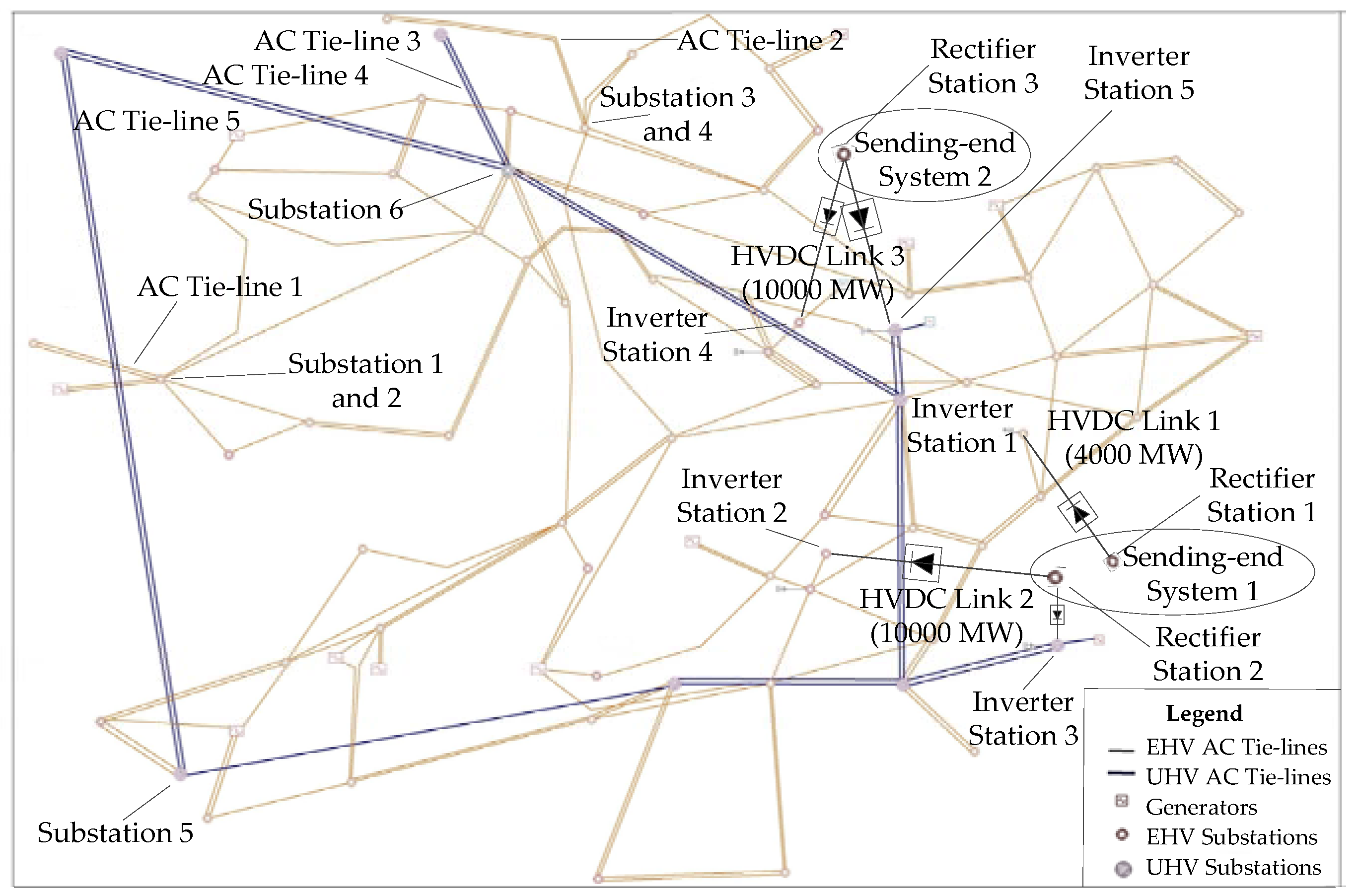
6.1. Test Power System

A provincial power system in China is simulated, which is a typical receiving-end system with multiple HVDC links and AC transmission lines integrated into it, as shown in Figure 3. There are three HVDC links, in which Links 2 and 3 are of hierarchical connection mode, i.e., the inverter stations are connected to two voltage-level buses. The rated power values of HVDC Links 1, 2 and 3 are 4000 MW, 10,000 MW and 10,000 MW, respectively. Besides, five double-circuit 500 kV and 1000 kV AC transmission lines from external power systems are connected. The reference value of system apparent power is set to be 100 MVA.

In practice, the DC power support values of HVDC systems are usually set with discrete levels. For instance, the DC power support values of Tian-Guang HVDC project in the China Southern Power Grid are set with five levels as 10%, 20%, 30%, 40% and 50% of the rated power [31]. The proposed strategy adopts the power system practice with the selection of the 10% step in the search space. The maximum value in percentage is generally limited to 50% for the reliability of the HVDC link. A quantity of reactive power must be absorbed for the secure operation of an HVDC link, which is usually 40–60% of the DC power value. Regular reactive power compensation devices equipped at rectifier and inverter stations (e.g., capacitors) can satisfy the requirement for normal operation states. Nevertheless, provision of DC power support by the HVDC link will pose extra reactive power compensation requirements.

To enhance reactive power support for the HVDC links, plenty SCs have been or will be installed at rectifier stations in the sending-end systems and inverter stations in the test power system (the receiving-end system). The number of SCs and their optimal locations should be planned accounting for technical and economic factors comprehensively [32]. The rated apparent power of a SC is 500 MVA. There are 6, 10 and 9 SCs installed close to Rectifier Stations 1, 2 and 3, respectively; Inverter Station 1 has 6 SCs; and each of Inverter Stations 2–5 has 5 SCs. The maximum adjustment percentage of excitation voltage reference value $V_{ref}$ for each SC is set to be 20%. Accounting for the reactive power support by the SCs, the maximum DC power support values in percentage for HVDC Links 1, 2 and 3 are 50%, 40% and 30%, respectively.

6.2. Effectiveness of OLPO for SCs

6.2.1. OLPO for SCs at Converter Station of Single HVDC Link

The leading phase operation for SCs is simulated to verify its effectiveness in supplementing an HVDC link to provide DC power support. The value of DC power support for HVDC Link 1 is set to be 30% of the rated value, i.e., 1200 MW.

The reactive power value Δ$Q_{r0}^{DC1}$ absorbed by SCs installed close to Rectifier Station 1 is set to be 3 p.u. and the search range of the reactive power value Δ$Q_{i0}^{DC1}$ absorbed by SCs installed close to Inverter Station 1 is set to be 1.5–3 p.u. Then, variations of DC power support values Δ$P_{dr0}^{DC1}$ and values of influence factor $q_{sc}^{DC1}$ can be obtained, which are listed in

Table 1. Reactive power values absorbed by SCs and variations of DC power support values for HVDC Link 1.

[Δ${\mathit{Q}}_{\mathit{r}0}^{\mathit{D}\mathit{C}1}$, Δ${\mathit{Q}}_{\mathit{i}0}^{\mathit{D}\mathit{C}1}$]/p.u.	Δ${\mathit{P}}_{\mathit{d}\mathit{r}0}^{\mathit{D}\mathit{C}1}$/p.u.	${\mathit{q}}_{\mathit{s}\mathit{c}}^{\mathit{k}}$	[Δ${\mathit{Q}}_{\mathit{r}0}^{\mathit{D}\mathit{C}1}$, Δ${\mathit{Q}}_{\mathit{i}0}^{\mathit{D}\mathit{C}1}$]/p.u.	Δ${\mathit{P}}_{\mathit{d}\mathit{r}0}^{\mathit{D}\mathit{C}1}$/p.u.	${\mathit{q}}_{\mathit{s}\mathit{c}}^{\mathit{k}}$
[3.0, 1.5]	−1.8 × 10−2	4 × 10−3	[3.0, 2.4]	−2.66 × 10−2	4.9 × 10−3
[3.0, 1.8]	−2.08 × 10−2	4.3 × 10−3	[3.0, 2.7]	−2.96 × 10−2	5.2 × 10−3
[3.0, 2.1]	−2.37 × 10−2	4.7 × 10−3	[3.0, 3.0]	−3.26 × 10−2	5.4 × 10−3

. As highlighted using boldface font in Table 1, values of [Δ$Q_{r0}^{DC1}$, Δ$Q_{i0}^{DC1}$] corresponding to the minimum value of $q_{sc}^{DC1}$ are obtained, which are the reactive power values to be absorbed by SCs installed close to the rectifier and inverter stations of HVDC Link 1.

As shown in Figure 4, with the leading phase operation for SCs implemented, the maximum reactive power output values for SCs can be decreased, which are 1.4 p.u. (decreased from 4.5 p.u.) at the rectifier station and 8.9 p.u. (decreased from 10.6 p.u.) at the inverter station. The control margin of SCs installed close to the rectifier and inverter stations are increased by 12% and 9%, respectively. Note that although the variations are only a small fraction of the total installed reactive power from the SCs, their marginal effect is significant.

6.2.2. OLPO for SCs at Converter Stations of Three HVDC Links

The OLPO model is solved for SCs installed close to the converter stations of three HVDC links in the test system. The model is built and solved by MATLAB/YALMIP and Gurobi.

Optimal reactive power values absorbed by SCs are ΔQ_i = [1.16, 1.66, 1.18, 0.5, 0.5] (p.u.) at Inverter Stations 1–5 and ΔQ_r = [2.32, 1.7, 0.9] (p.u.) at Rectifier Stations 1–3. Variations of DC power support values ΔP_dr0 for five HVDC infeeds in the receiving-end system can be obtained, which are ΔP_dr0 = [0.0723, 0.0693, 0.0682, 0.0714, 0.0716] (p.u.). The maximum difference among the values of ΔP_dr0 is 0.0041 p.u. (0.41 MW).

6.3. Selection of HVDC Links Participating in DC Power Support

HVDC links participating in DC power support are selected by using DC power support factors K_r for three rectifier stations in the two sending-end systems and K_i for five inverter stations in the receiving-end system. The values of K_r and K_i are listed in

Table A1. K_r for rectifier stations of non-fault HVDC links in sending-end systems.

Fault HVDC Link	Kr for Non-Fault HVDC Links
	HVDC Link 1	HVDC Link 2	HVDC Link 3
HVDC Link 1	N/A	0.3273	0
HVDC Link 2	0.2199	N/A	0
HVDC Link 3	0	0	N/A

and

Table A2. K_i for inverters stations of non-fault HVDC links in receiving-end systems.

Inverter Stations/Substations of Fault HVDC Links/AC Tie-Lines		Inverter Stations of Non-fault HVDC Links
		Inverter Station 1	Inverter Station 2	Inverter Station 3	Inverter Station 4	Inverter Station 5
Ki	Inverter Station 1	N/A	0.5024	0.5461	0.4336	0.4668
	Inverter Station 2	0.4207	N/A	N/A	0.3267	0.4780
	Inverter Station 3	0.4035	N/A	N/A	0.3550	0.7097
	Inverter Station 4	0.4288	0.2894	0.3567	N/A	N/A
	Inverter Station 5	0.4080	0.3750	0.6301	N/A	N/A
	Substation 1	0.1214	0.0796	0.1142	0.1027	0.0913
	Substation 2	0.1214	0.0796	0.1142	0.1027	0.0913
	Substation 3	0.1600	0.1017	0.1374	0.1136	0.1094
	Substation 4	0.1600	0.1017	0.1374	0.1131	0.1094
	Substation 5	0.2251	0.1852	0.3047	0.1229	0.2077
	Substation 6	0.2050	0.1502	0.2390	0.1235	0.1961

, respectively.

To compute the values of K_r and K_i, the MIIF and MESCR indices are required. First, values of the MIIF index is obtained according to Equation (9) by using the perturbation approach where MIIF_rDC3-DC1, MIIF_rDC3-DC2, MIIF_rDC1-DC3 and MIIF_rDC2-DC3 are 0 due to the large electrical distances between Rectifier Stations 1 and 3 and that between Rectifier Stations 2 and 3. Then, values of the MESCR index is calculated according to Equation (11).

For any disturbance scenario, HVDC links participating in DC power support can be determined. For instance, a disturbance scenario is the situation that HVDC Link 2 is bipolar blocking, which is termed as Scenario 1. Under Scenario 1, values of K_rDC2-DC1 and K_rDC2-DC3 in the sending-end systems are 0.2199 and 0, respectively. Therefore, the rank order of non-fault HVDC links is HVDC Link 1 followed by Link 3. For Scenario 2 that HVDC Link 3 is bipolar blocking, the rank order of non-fault HVDC links cannot be determined according to K_r in the sending-end systems since values of K_rDC3-DC1 and K_rDC3-DC2 are both 0. The values of K_i in the receiving-end system are used instead. The value of K_iDC3-DC1 is 0.8368 (=0.4288 + 0.4080) and K_iDC3-DC2 is 1.6512 (=0.2894 + 0.3567 + 0.3750 + 0.6301). Thus, the rank order of non-fault HVDC links is HVDC Link 2 followed by Link 1. Since the maximum sum values of DC power support for Scenarios 1 and 2 are 5000 MW and 6000 MW, respectively, both of which are smaller than the values of power loss 10,000 MW for the two scenarios, all non-fault HVDC links are selected to participate in DC power support for both scenarios.

6.4. Optimization of DC Power Support Values

6.4.1. Search Space of DC Power Support Values

To reduce the computational burden for the test system, the search space of DC power support values is expressed as combinations of DC power support values in percentage for the selected HVDC links accounting for the levels and limits of DC power support. Combinations of DC power support values in percentage for Scenarios 1 and 2 are listed in

Table A3. Combinations of DC power support values when HVDC Link 2 or 3 is bipolar blocking.

Combinations of DC Power Support Values for [DC1, DC3] When HVDC Link 2 Is Bipolar Blocking/%				Combinations of DC Power Support Values for [DC1, DC3] When HVDC Link 3 Is Bipolar Blocking/%
[0, 0]	[0, 10]	[0, 20]	[0, 30]	[0, 0]	[0, 10]	[0, 20]	[0, 30]	[0, 40]
[10, 10]	[10, 10]	[10, 20]	[10, 30]	[10, 10]	[10, 10]	[10, 20]	[10, 30]	[10, 40]
[20, 10]	[20, 10]	[20, 20]	[20, 30]	[20, 10]	[20, 10]	[20, 20]	[20, 30]	[20, 40]
[30, 10]	[30, 10]	[30, 20]	[30, 30]	[30, 10]	[30, 10]	[30, 20]	[30, 30]	[30, 40]
[40, 10]	[40, 10]	[40, 20]	[40, 30]	[40, 10]	[40, 10]	[40, 20]	[40, 30]	[40, 40]
[50, 10]	[50, 10]	[50, 20]	[50, 30]	[50, 10]	[50, 10]	[50, 20]	[50, 30]	[50, 40]

. A part of combinations can prevent the test system from losing stability, which are highlighted in Table A3 by using the boldface font. The criteria for the system losing stability are differences among rotor angles of generators are larger than 500, voltages of buses are smaller than 0.7 p.u. lasting for more than one second or frequency is smaller than 45 Hz lasting for more than one second.

The AVREF model is used to coordinately adjust V_ref for SCs installed close to the rectifier and inverter stations and ensure DC power to achieve the target values. For example, under Scenario 1, the combination [50, 30] (%) of DC power support values should be achieved by adjusting V_ref for SCs, in which the target DC power support values for HVDC Link 1 and Link 3 are 2000 (=4000 × 50%) MW and 3000 (=10,000 × 30%) MW, respectively. As shown in Figure 5a, with adjusting V_ref, the DC power support value for HVDC Link 1 does achieve 2000 MW (DC power is increased from 4000 MW to 6000 MW). However, the DC power support value can only approach 1500 MW without adjusting V_ref. As shown in Figure 5b, the DC power support value for HVDC Link 3 can actually achieve 3000 MW with adjusting V_ref and can only approach 2000 MW without adjusting V_ref.

6.4.2. Optimal Combination of DC Power Support Values

The optimal combination of DC power support values for any disturbance scenario is obtained by employing the comprehensive stability margin index η. First, the combinations preventing the system from losing stability are extracted. Then, the values of transient stability margin index η_t and the frequency security margin index η_f are computed for each of the combinations. To derive the comprehensive stability margin index η, a normalization process is used through which the values of η_t and η_f are normalized and fall into the range between 0 and 1. The weight coefficients in Equation (18), i.e., h_t, h_f, $z_t^1$, $z_t^2$ and z_f are set to be 0.5 and binary tables for Scenarios 1 and 2 are [49.8 Hz, 3 s] and [49.8 Hz, 5 s], respectively. As shown in

Table 2. Combinations of DC power support values and quantitative indices for scenarios.

Scenario 1: HVDC Link 2 Is Bipolar Blocking
Combinations [DC1, DC3] (%)	ηt	ηf	η	Combinations [DC1, DC3] (%)	ηt	ηf	η
[50, 20]	1	0.14	0.57	[30, 30]	0.14	0.50	0.32
[50, 30]	0.85	1	0.93	[20, 30]	0.00	0	0.00
[40, 30]	0.65	0.90	0.78
Scenario 2: HVDC Link 3 Is Bipolar Blocking
Combinations [DC1, DC2] (%)	ηt	ηf	η	Combinations [DC1, DC2] (%)	ηt	ηf	η
[50, 20]	0.87	0.47	0.67	[0, 40]	0.85	0	0.43
[10, 30]	1.00	0.44	0.72	[10, 40]	0.62	0.51	0.57
[20, 30]	0.87	0.46	0.67	[20, 40]	0.54	0.55	0.55
[30, 30]	0.56	0.49	0.53	[30, 40]	0.36	0.63	0.50
[40, 30]	0.28	0.51	0.40	[40, 40]	0.05	0.78	0.42
[50, 30]	0.18	0.56	0.37	[50, 40]	0.00	1	0.50

, the value of η corresponding to each combination of DC power support values is the sum of the normalized values of η_t and η_f.

The optimal combination of DC power support values for each scenario can be obtained, which corresponds to the largest value of the comprehensive stability margin index η, as highlighted in Table 2 using the boldface font. The optimal combination is [50, 30] (%) for Scenario 1 and is [10, 30] (%) for Scenario 2. For Scenario 1, DC power support values provided by HVDC Links 1 and 3 are 2000 MW and 3000 MW, respectively, which can effectively compensate the power loss caused by the bipolar blocking condition of HVDC Link 2. The DC power support provided by HVDC Links 1 and 2 also contributes greatly to balance the power loss for Scenario 2.

The transient stability margin index η_t is a correct indicator quantifying the impacts of DC power support to the sending-end systems. For Scenario 1, the increase of DC power support from HVDC Link 1 is positive to the transient stability since HVDC Link 1 is in the same sending-end system with HVDC Link 2 and it can mitigate the negative effect caused by the bipolar blocking condition of HVDC Link 2. As shown in Table 2, the value of η_t for the combination of [50, 30] (%) is larger than that of [40, 30] (%), which is consistent with the positive impact of HVDC Link 1. However, the increase of DC power support from HVDC Link 3 is negative to the transient stability since HVDC Link 3 is in a distinct sending-end system asynchronously interconnected with the one in which HVDC Link 2 is sited and it will worsen the situation. The negative impact of HVDC Link 3 can be exemplified by that the value of η_t for the combination of [50, 30] (%) is smaller than that of [50, 20] (%).

The impacts of DC power support to the receiving-end systems can be appropriately reflected by the frequency security margin index η_f. The value of η_f is positively related to the increase of DC power support from HVDC links since the power loss caused by the fault condition can be balanced by the DC power support and the frequency deviation in the receiving-end systems will be corrected. As shown in Table 2, the value of η_f for the combination of [50, 30] (%) is the largest for Scenario 1 while the combination of [50, 40] (%) takes the largest value of η_f for Scenario 2. It is clear that the above two combinations are of the largest sum values of DC power support compared with the other combinations for Scenarios 1 and 2, respectively.

6.4.3. Optimal Load Shedding

The values of the frequency security margin index η_f corresponding to Scenarios 1 and 2 are −0.9122 and −0.8490 (without normalization), respectively, which are much smaller than the requirement. The load shedding step is required to increase the frequency security margin by solving the OLS model. Parameters of the OLS model are as follows

• There are 17 load shedding areas in the receiving-end system and the upper limit of the shedding value in each area is set to be 15% of the load level in the area.
• ε is set to be 1 × 10⁻³.
• Load shedding is actuated at 0.2 s after HVDC Link 2 or 3 is bipolar blocking.

The optimal solutions for the two scenarios are 6415 MW and 6038 MW, respectively. Dynamic simulations are conducted to verify the efficacy of the load shedding step. As shown in Figure 6, the frequency security of the test system is enhanced dramatically by load shedding, which is just within the security range of [49.8 Hz, 50.2 Hz] for the two scenarios. Nevertheless, the frequency security of the test system is significantly degraded without actuating the load shedding step. The results demonstrate the supplementary effect of the load shedding to the DC power support.

7. Conclusions

A coordinated DC power support strategy for multi-infeed HVDC systems is proposed in this paper. The DC power of HVDC links can be effectively modulated to achieve the set values while ensuring the power system stability. The optimal leading phase operation and adjustment of excitation voltage reference values of SCs are solved by the proposed OLPO and AVREF models, which can provide the required dynamic reactive power. The HVDC links participating in DC power support are ranked and selected according to the DC power support factor. The comprehensive stability margin index is used to obtain optimal DC power support values of the participating links. The optimal load shedding can supplement the DC power support to ensure the frequency security of the receiving-end system. Simulation results of a provincial power system in China demonstrate the effectiveness and performance of the proposed DC power support strategy.

References

1. Hwang, S.; Lee, J.; Jang, G. HVDC-system-interaction assessment through line-flow change-distribution factor and transient-stability analysis at planning stage. Energies 2016, 9, 1068. [Google Scholar] [CrossRef]
2. Liu, C.; Zhao, Y.; Li, G.; Udaya, D. Design of LCC HVDC wide-area emergency power support control based on adaptive dynamic surface control. IET Gener. Transm. Distrib. 2017, 11, 3236–3245. [Google Scholar] [CrossRef]
3. Harnefors, L.; Johansson, N.; Zhang, L.; Berggren, B. Interarea oscillation damping using active-power modulation of multiterminal HVDC transmissions. IEEE Trans. Power Syst. 2014, 29, 2529–2538. [Google Scholar] [CrossRef]
4. Rahman, H.; Khan, B.H. Stability improvement of power system by simultaneous AC–DC power transmission. Electr. Power Syst. Res. 2008, 78, 756–764. [Google Scholar] [CrossRef]
5. Sun, Y.; Li, X.; Su, M.; Wang, H.; Dan, H.; Xiong, W. Indirect matrix converter-based topology and modulation schemes for enhancing input reactive power capability. IEEE Trans. Power Electron. 2015, 30, 4669–4681. [Google Scholar] [CrossRef]
6. Wang, K.; Yang, S.; Yao, J. Multi-circuit HVDC system emergency DC power support with reactive control. In Proceedings of the 2011 IEEE/PES Power Systems Conference and Exposition, Phoenix, AZ, USA, 20–23 March 2011; pp. 1–5. [Google Scholar]
7. Teleke, S.; Abdulahovic, T.; Thiringer, T.; Svensson, J. Dynamic performance comparison of synchronous condenser and SVC. IEEE Trans. Power Deliv. 2008, 23, 1606–1612. [Google Scholar] [CrossRef]
8. Kirby, N.M.; Marken, P.E.; Paradis, M.; Wang, P.; Plowright, I.; Moon, H.; Ingemansson, D.; Mendis, R.; Mehraban, B. Extending their lifetimes: Keeping HVDC and FACTS installations in service longer. IEEE Power Energy Mag. 2016, 14, 57–65. [Google Scholar] [CrossRef]
9. Zhang, L.; Harnefors, L.; Nee, H.P. Interconnection of two very weak AC systems by VSC-HVDC links using power-synchronization control. IEEE Trans. Power Syst. 2011, 26, 344–355. [Google Scholar] [CrossRef]
10. Wang, C.; Wang, H.; Xu, G. System voltage regulation of power grid based on synchronous generator’s leading phase operation. In Proceedings of the 2010 China International Conference on Electricity Distribution, Nanjing, China, 12–16 September 2010; pp. 1–4. [Google Scholar]
11. Wang, L.; Li, W.; Huo, F.; Zhang, S.; Guan, C. Influence of underexcitation operation on electromagnetic loss in the end metal parts and stator step packets of a turbogenerator. IEEE Trans. Energy Convers. 2014, 29, 748–757. [Google Scholar] [CrossRef]
12. Cui, T.; Lin, W.; Sun, Y.; Xu, J.; Zhang, H. Excitation voltage control for emergency frequency regulation of island power systems with voltage-dependent loads. IEEE Trans. Power Syst. 2016, 31, 1204–1217. [Google Scholar] [CrossRef]
13. Masood, N.A.; Yan, R.; Saha, T.K.; Bartlett, S. Post-retirement utilisation of synchronous generators to enhance security performances in a wind dominated power system. IET Gener. Transm. Distrib. 2016, 10, 3314–3321. [Google Scholar] [CrossRef]
14. Wang, X.; Zhang, H.; Xu, Z.; Weng, H.; Xu, F. Emergency power support for multiple DCs based on trajectory sensitivity. Electr. Power Automat. Equip. 2014, 34, 86–91. [Google Scholar]
15. Rafael, Z.; Thierry, V.; Federico, M.; Antonio, J. Securing transient stability using time-domain simulations within an optimal power flow. IEEE Trans. Power Syst. 2010, 25, 243–253. [Google Scholar]
16. Vu, T.L.; Turitsyn, K. Lyapunov functions family approach to transient stability assessment. IEEE Trans. Power Syst. 2016, 31, 1269–1277. [Google Scholar] [CrossRef]
17. Xu, Y.; Dong, Z.; Zhang, R.; Xue, Y.; David, J. A decomposition-based practical approach to transient stability-constrained unit commitment. IEEE Trans. Power Syst. 2015, 30, 1455–1464. [Google Scholar] [CrossRef]
18. Liu, Z.Y.; Liu, C.R.; Li, G.Y.; Liu, Y.; Liu, Y.L. Impact study of PMSG-based wind power penetration on power system transient stability using EEAC theory. Energies 2015, 8, 13419–13441. [Google Scholar] [CrossRef]
19. Zhang, H.; Li, C.; Liu, Y. Quantitative frequency security assessment method considering cumulative effect and its applications in frequency control. Int. J. Electr. Power Energy Syst. 2015, 65, 12–20. [Google Scholar] [CrossRef]
20. Xu, X.; Zhang, H.; Li, C.; Liu, Y.; Li, W.; Terzija, V. Optimization of the event-driven emergency load-shedding considering transient security and stability constraints. IEEE Trans. Power Syst. 2017, 32, 2581–2592. [Google Scholar] [CrossRef]
21. Lin, Q.; Li, X.Y.; Wang, X. Multi-DC emergency power support strategy based on DC comprehensive support factors. East China Electr. Power 2013, 41, 1431–1435. [Google Scholar]
22. Zhao, R.; Zhang, Y.; Li, X.; Chen, H.; He, Y. The research on the emergency DC power support strategies of Deyang-Baoji HVDC project. In Proceedings of the 2011 Asia-Pacific Power and Energy Engineering Conference, Wuhan, China, 25–28 March 2011; pp. 1–4. [Google Scholar]
23. Liu, X.; Xie, H.; Wang, H.; Wang, H.; Wang, Z.; Lv, J. Emergency DC power support in parallel AC/DC power system. In Proceedings of the 2013 International Conference on Mechatronics and Automatic Control Systems, Hangzhou, China, 10–11 August 2013; pp. 525–532. [Google Scholar]
24. Daryabak, M.; Filizadeh, S.; Jatskevich, J.; Davoudi, A.; Saeedifard, M.; Sood, V.K.; Martinez, J.A.; Aliprantis, D.; Cano, J.; Mehrizi-Sani, A. Modeling of LCC-HVDC systems using dynamic phasors. IEEE Trans. Power Deliv. 2014, 29, 1989–1998. [Google Scholar] [CrossRef]
25. Li, Y.; Luo, L.; Rehtanz, C.; Sven, R.; Liu, F. Realization of reactive power compensation near the LCC-HVDC converter bridges by means of an inductive filtering method. IEEE Trans. Power Deliv. 2012, 27, 3908–3923. [Google Scholar] [CrossRef]
26. Aik, D.L.H.; Andersson, G. Analysis of voltage and power interactions in multi-infeed HVDC systems. IEEE Trans. Power Deliv. 2013, 28, 816–824. [Google Scholar] [CrossRef]
27. Liao, S.; Yao, W.; Ai, X.; Wen, J.; Liu, Q.; Jiang, Y.; Zhang, J.; Tu, J. An improved multi-infeed effective short-circuit ratio for AC/DC power systems with massive shunt capacitors installed. Energies 2017, 10, 396. [Google Scholar] [CrossRef]
28. Saunders, C.S.; Alamuti, M.M.; Taylor, G.A. Transient stability analysis using potential energy indices for determining critical generator sets. In Proceedings of the 2014 IEEE PES General Meeting, National Harbor, MD, USA, 27–31 July 2014; pp. 1–5. [Google Scholar]
29. Jain, A.K. Data clustering: 50 years beyond K-means. Pattern Recognit. Lett. 2010, 31, 651–666. [Google Scholar] [CrossRef] [Green Version]
30. Luo, C.; Yang, J.; Sun, Y.Z. Risk assessment of power system considering frequency dynamics and cascading process. Energies 2018, 11, 422. [Google Scholar] [CrossRef]
31. Yang, K.; Peng, S.; Dong, S.; Bin, L. Research on stability control strategy for island system of HVDC. In Proceedings of the 3rd International Conference on Mechanical Engineering and Intelligent Systems, Windsor, UK, 29–30 September 2016; pp. 694–699. [Google Scholar]
32. Zhang, Y.; Huang, S.; Schmall, J.; Conto, J.; Billo, J.; Rehman, E. Evaluating system strength for large-scale wind plant integration. In Proceedings of the 2014 IEEE PES General Meeting, National Harbor, MD, USA, 27–31 July 2014; pp. 1–5. [Google Scholar]
Figure 1. Schematic diagram of a multi-infeed HVDC system.
Energies 11 01637 g001
Figure 2. Flowchart of DC power support strategy.
Energies 11 01637 g002
Figure 3. Topological structure diagram of provincial power system.
Energies 11 01637 g003
Figure 4. Effectiveness of the leading phase operation for SCs installed close to converter stations of HVDC Link 1.
Energies 11 01637 g004
Figure 5. Effectiveness of adjusting Vref during DC power support. (a) DC power curves of HVDC Link 1 for Scenario 1; and (b) DC power curves of HVDC Link 3 for Scenario 1.
Energies 11 01637 g005
Figure 6. Frequency curves for Scenarios 1 and 2.
Energies 11 01637 g006