Article

Experimental Comparison of Three Real-Time Optimization Strategies Applied to Renewable/FC-Based Hybrid Power Systems Based on Load-Following Control

1
Faculty of Electronics, Communications and Computers Science, University of Pitesti, 110040 Pitesti, Romania
2
Doctoral School, University Politehnica of Bucharest, 061071 Bucharest, Romania
*
Author to whom correspondence should be addressed.
Energies 2018, 11(12), 3537; https://doi.org/10.3390/en11123537
Submission received: 19 November 2018 / Revised: 13 December 2018 / Accepted: 17 December 2018 / Published: 19 December 2018
(This article belongs to the Special Issue Sustainable Energy Systems)

Abstract

:
Besides three different real-time optimization strategies analyzed for the Renewable/Fuel Cell Hybrid Power Systems (REW/FC-HPS) based on load-following (LFW) control, a short but critical assessment of the Real-Time Optimization (RTO) strategies is presented in this paper. The advantage of power flow balance on the DC bus through the FC net power generated using the LFW control instead of using the batteries’ stack is highlighted in this study. As LFW control consequence, the battery operates in charge-sustained mode and many advantages can be exploited in practice such as: reducing the size of the battery and maintenance cost, canceling the monitoring condition of the battery state-of-charge etc. The optimization of three FC-HPSs topologies based on appropriate RTO strategy is performed here using indicators such as fuel economy, fuel consumption efficiency, and FC electrical efficiency. The challenging task to optimize operation of the FC-HPS under unknown profile of the load demand is approached using an optimization function based on linear mix of the FC net power and the fuel consumption through the weighting coefficients knet and kfuel. If optimum values are chosen, then a RTO switching strategy can improve even further the fuel economy over the entire range of load.

Graphical Abstract

1. Introduction

In renewable energy Hybrid Power Systems (HPS) applications, the generation power is usually intermittent and variable, the load power is also dynamic with the daily energy consumption, such as in Fuel Cell Hybrid Power Systems (FC-HPS), wind turbine farms, and solar arrays.
The main objective for the FC-HPS [1,2,3,4] and other hybrid energy systems [5,6,7] is to efficiently operate these systems based on rule-based and optimization-based strategies proposed in the last years [8,9]. As it is known, the deterministic rule-based strategy is already available in the market due to their reduced complexity in implementation, but this type of strategy cannot find the optimum solution [10], so the research interest has switched to optimization-based Real-Time Optimization (RTO) strategies, even if the complexity increases [1,11]. These strategies can find and track in real-time the optimal solution or a suboptimal solution close to it [7,12]. The RTO strategies usually use optimization algorithms such as the Extremum Seeking (ES) algorithms [13,14], the Equivalent Consumption Minimization Strategy (ECMS) [15,16], the intelligent algorithms [17,18,19], the Model Predictive Control (MPC) schemes [20,21], and so on [22,23,24,25,26]. From these RTO-strategies, the ECMSs based on Pontryagin’s Minimum Principle (PMP) [26,27] or Dynamic Programming (DP) are most used for FC-HPS [10].
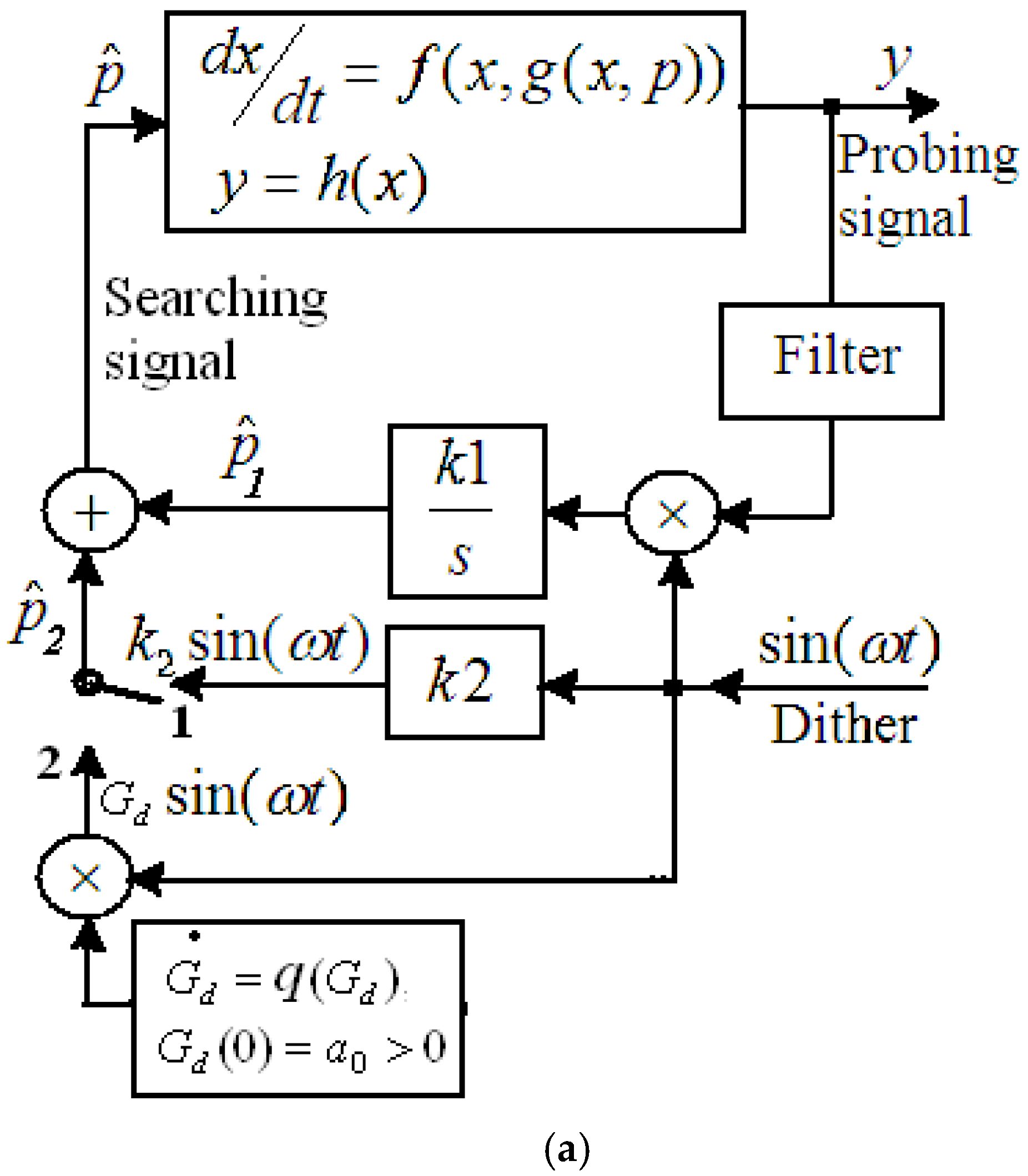
Different ES-based RTO strategies based on classical [28,29], modified [30,31], and advanced [13,14,32,
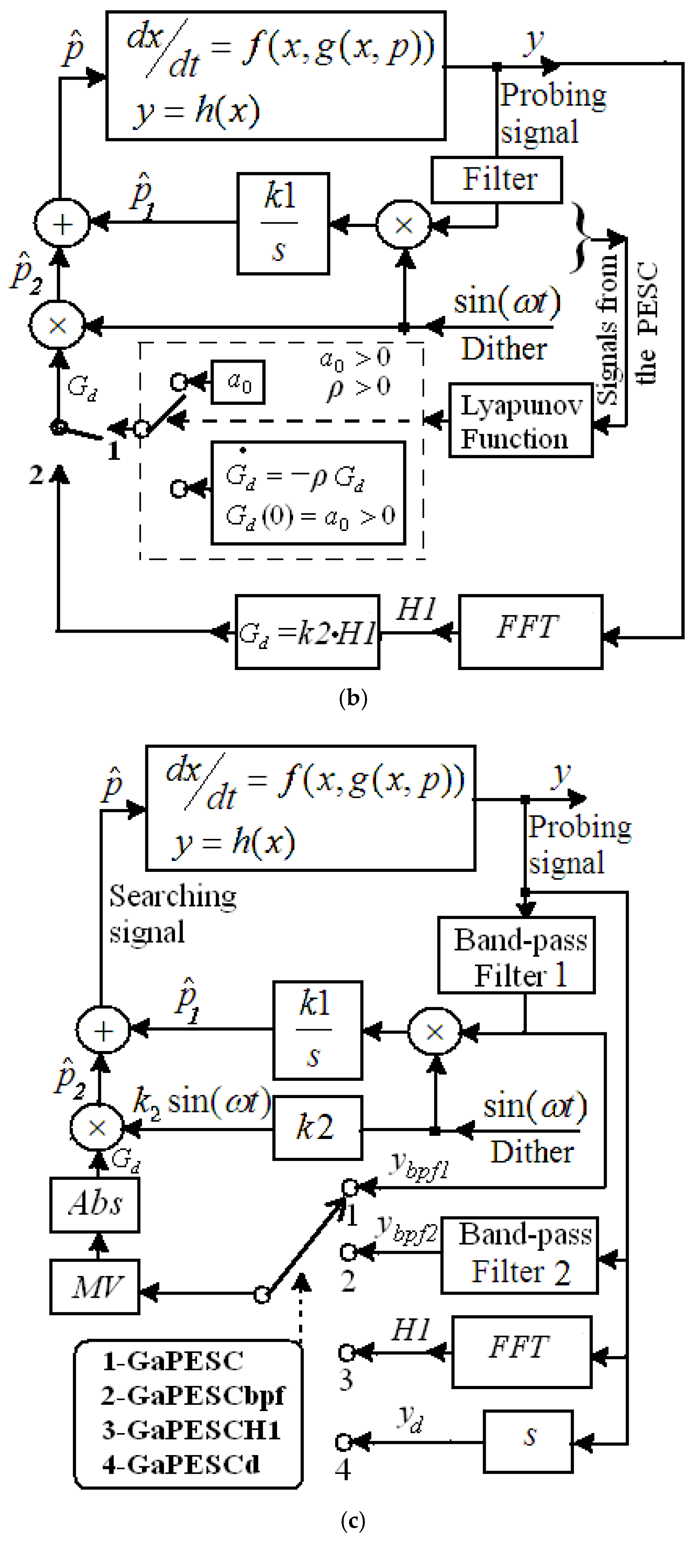
33] ES algorithms were proposed recently to optimally operate the FC-HPS. The modified ES algorithm improves the tracking robustness compared to conventional ES algorithm due to tge use of a Band-Pass Filter (BPF) to process more power harmonics into the seeking signal [30,31]. The advanced ES algorithm improves the tracking accuracy compared to modified ES algorithm by using modulation of the dither amplitude with the magnitude of first harmonics of the FC power. Furthermore, the FC ripple power decreases around the Maximum Efficiency Point (MEP), which is faster found [32]. A comparative study of the ES-based RTO strategies is presented in [33,34]. The global ES (GES) algorithm tracks the global Maximum Power Point (MPP) instead of local MPP, improving with more than 30% the efficiency of the photovoltaic (PV) system [35,36,37]. The GES algorithm [35] uses two BPFs instead of one BPF [36]. The design rules for the GES algorithms are detailed in [37].
PV arrays, wind turbines and battery stacks generate the needed load power in renewable energy systems and a design to comply the power flow balance on the Direct Current (DC) bus could oversize the battery stack due to the high dynamics of the load profile and variability of the available renewable energy. This issue can be solved by using the Load-Following (LFW) control of the FC boost converter [38] to compensate the power flow balance on the DC and the battery will operate in charge sustaining mode, which means reducing the size of the batteries stack. Thus, considering additionally the reduction of maintenance costs, the overall cost of FC-HPS remains within the same range as the battery-based HPS cost. Furthermore, for example, the LFW control is simpler to be implemented compared to ES-based RTO routine to rescale the air flow rate (AirFr) of the Proton Exchange Membrane FC (PEMFC) system or other energy management strategies based on states’ diagram [39]. Different RTO-strategies have been proposed for FC-HPS to improve the free air breathing of PEMFC system through the MEP [40] or MPP [41] tracking techniques, or based on other robust control techniques [42] which are analyzed and compared in [43]. The MPP tracking technique improves the tracking accuracy of a photovoltaic/FC-HPS by simultaneously optimizing both the PV and FC systems [44]. The renewable HPS architecture requires a FC system and electrolyzer to store the hydrogen in order to mitigate the variability of the renewable power, but a regenerative FC stack could solve this issue in one device [45,46].
Besides the LFW control of the FC system [38], other different algorithms can be used as well [46], such as artificial intelligent algorithms [47] based on neural networks [48], genetic algorithms [49], or data fusion approach [50]. The combinatorial techniques [51], the Model Reference Adaptive Control (MRAC) [52], the metaheuristic approaches [53], the prediction of the load demand [54], and ECMSs techniques [55] are other methods proposed to optimize the operation of the FC-HPS.
The static feed-forward (sFF) control of the FC system was first implemented in practice [56], but many other control algorithms for air compressor systems have been designed based on the Hardware-in-Loop System (HILS) technique [56,57,58,59,60,61,62,63,64,65,66,67]. The HILS-based second order sliding mode controller implemented in a commercial twin screw air compressor sub-optimally controls the air feed system [57] avoiding oxygen starvation and the compressor surge phenomenon using the load governor method and constrained extremum technique [58]. Thus, the AirFr of the PEMFC system can be optimally control by a second order sliding mode control [59]. The better mitigation of load ripples and pulses on PEMFC operation can be ensured using a disturbance rejection control [60] or a differential flatness approach [61] compared to a classic Proportional–Integral (PI) controller [56]. Also, by appropriate control of the cathode system, the lifetime of the PEMFC system could be increased to 25 years in next decade [62]. The Linear Quadratic Regulator (LQR)/Linear Quadratic Gaussian (LQG) control maintains the best oxygen stoichiometry in PEMFC systems [63], but other optimal control solutions for the AirFr are proposed in literature based on ES algorithm [32], feed-forward fuzzy Proportional Integral Derivative (PID) control [64], optimal PID plus fuzzy controller [65], time delay control [66], and adaptive control [67].
Besides control for air systems, other control solutions to improve the fuel economy of the fuel system were proposed [43] such as global optimization methods based on fuzzy logic [68] and genetic [49] algorithms, adaptive algorithms such as adaptive fuzzy control [69] and adaptive Energy Management Strategy (EMS) [70], but most of them require prior knowledge of the driving cycle. Furthermore, these algorithms are difficult to implement in RTO strategies due to its computational complexity; so, the research field of designing efficient and simple RTO strategies for FC-HPS still remains challenging.
In this paper, using Matlab-Simulink version 2013®, the performance of three LFW control-based FC-HPS topologies is compared considering the optimization loop implemented to size the FC boost converter (the new RTO3 strategy), AirFr regulator (the RTO2 strategy [71]), or Fuel Flow rate (FuelFr) regulator (the RTO1 strategy [72]). All the topologies use one optimization loop and LFW control to mitigate the variability of the load demand and renewable energy on battery State-Of-Charge (SOC). The performance of the proposed RTO strategies is compared to the sFF reference strategy under same unknown profile of the Load Cycle (LC) based on the following indicators: (1) the FC net power, (2) the fuel consumption efficiency, (3) the electrical efficiency of the FC system, and (4) the total fuel consumption. The optimization function used in this study is designed to reduce the total fuel consumption under unknown LC, being a linear weighted function of the FC energy efficiency and the fuel consumption efficiency through the weighting coefficients knet and kfuel. The GES algorithm is used to find in real-time the global maximum of the optimization function [35].
Design of the weighting coefficients knet and kfuel will improve the fuel economy of a FC vehicle under unknown LC. Thus, the performance is estimated for all three FC-HPS topologies compared to the sFF strategy using same profile for the constant and variable load demand. The RTO strategies for the FC-HPS topologies clearly differ in the place where the optimization is performed and the LFW control is applied (see Table 1). Finally, considering the obtained performance, some guiding design rules to choose the switching RTO strategy are given.
The paper is organized as follows: optimization objectives and algorithms for FC-HPS based on the extremum seeking algorithm are very briefly mentioned in Section 2. The LFW control-based RTO strategies with specific optimization loop are designed in Section 3 considering the power flow balance at the DC bus. The results for all three RTO strategies are presented in Section 4 compared to the sFF strategy for constant and variable load, without and with renewable energy support. Section 5 discusses the results obtained and the last section concludes the paper.

2. Optimization Objectives and Algorithms

The RTO switching control strategies proposed in this paper will be implemented based on the theory of problem optimization applied in many engineering applications.

2.1. Optimization Algorithms

Optimization of the FC-HPS is the real-time process of searching for the set of values in the search range, called the optimal value (or the optimum) and which must be very close to the global extreme of the optimization function, so besides high tracking and searching accuracy [35,36], the global search feature of the optimization algorithm must have a 100% hit count and to have a good robustness to different perturbations into the system (such variations of the load demand and renewable power) [5,6,73]. The input vector will continuously seek the new optimum in the searching range due to changes in the requested load demand and available renewable power which set the needed FC power under LFW control. If some stationary regimes could appear, then the FC ripple current must be minimum [35,36,74]. The FC net power PFCnet = f(AirFf, FuelFr) has an optimum called MEP and many other peaks on the plateau around the MEP [1], but 99.9% searching accuracy and less than 1% searching resolution help the GES algorithm to discern the MEP from them [37], so the ES algorithm [37] was used in this study due to its reported performance features and location and tracking of the MEP in one search stage (less than 10 dither periods, which, for example, means less than 0.01 s for a 1000 Hz sinusoidal dither). The firmware-based global MPP tracking algorithms proposed in literature operate in two stages, so their tracking time results are higher compared to the GES algorithm. The tracking accuracy (Tacc) and searching resolution (SR) are defined as follows [37]:
S R = min i | y G M P P y L M P P i | y G M P P 100 [ % ]
T a c c = y G M P P y G M P P 100 [ % ]
where yGMPP, yLMPP < yGMPP, and y*GMPP < yGMPP are the global extreme, the local maxima, and the value tracked with the GMPPT algorithm.
Furthermore, the GES algorithm [37] does not need complicated and periodic tuning of the parameters [75], so it is simple to design and implement [76], but ultimately the performance of all optimization algorithms depend on the to optimization objectives and constraints defined for a specific FC-HPS.

2.2. Optimization Objectives and Constraints

The optimization procedure usually follows the following steps: identifying and defining the optimization problem, designing the model, simulating and evaluating the model, refine the problem, and finally implementing optimal solution. The optimization objectives are in general contradictory, so multi optimization functions are proposed instead of one optimization function [77], integrating the constraints by penalty function related to battery SOC level [78,79].
The FC-HPS optimization can be generally defined as follows:
  • Maximize:
    f ( x , A i r F r , F u e l F r , P L o a d ) = k n e t P F C n e t + k f u e l F u e l e f f
  • Subject to FC-HPS dynamics:
    x ˙ = g ( x , A i r F r , F u e l F r , P L o a d ) , x X
  • and battery SOC constraints:
    S O C min < S O C < S O C max
In Equations (3a–c) PLoad, knet and kfuel represent the disturbance input, respectively weighting coefficients that will be switched according to the objectives defined in real-time during an unknown LC [80].
For example, the FC vehicle will adapt the parameters of the used optimization function considering the available on-line information about the route profile or the requests from as inputs of the Energy Management Unit (EMU) [81,82] as follows: the FC net power must be maximized if the FC vehicle climbs up a hill, the fuel economy must be maximized if the FC vehicle runs smoothly on the highway, the fuel consumption efficiency must be maximized if the communication unit informs the EMU that the fuel tank is almost empty based on signaling sensors, but a fuel station is close to the current position of the FC vehicle.
The number of sensors must be reduced at minimum for the FC-HPS based on Renewable Energy Systems (RES) by using adaptive algorithms to improve the fuel economy for plug-in FC vehicles [83] or grid-connected FC-HPS [84], which usually use many decision variables and constraints as inputs for the EMU such as [85]: the number of energy source units (FC systems, PV panels, wind turbines (WT), batteries, power storage devices, electrolyzers), RES potential (insolation and wind speed in installation area), technical characteristics (PV panel position, WT height), battery characteristics (SOCmin, SOCmax), hydrogen storage availabilities (tank volume, electrolyzer capacity), type of power storage devices (superconducting magnetic energy storage or SMES, flywheel energy storage or FES, ultracapacitors) and so on [1,4]. The constraints to design the FC-HPS of a FC vehicle are clearly related to available space and weight limitations, lifetime and safe operation of the FC system and batteries stack, maintenance cost, and so on [83], so an optimization problem involving multiple objectives such as technical, economic, and environmental objectives must be a combination of the conflicting performance indicators to be easy implemented [1,45]. Besides the fuel economy (or total fuel consumption: F u e l T = F u e l F r ( t ) d t ) as general performance indicator, other performance indicators can be integrated in the optimization function depending of application and load profile [86], but also by the environment conditions due to emplacement of the FC-HPS in different places situated on worldwide [87]. For example, fuel economy, lithium battery size and powertrain system durability, and, respectively, fuel economy and power efficiency are linearly mixed in the optimization function used in [88,89]. The performance indicators that could be used are as follows: the fuel consumption efficiency ( F u e l e f f = P F C n e t F u e l F r ) , the FC electrical efficiency ( η s y s = P F C n e t P F C ) , and the efficiency of hydrogen consumption ( e f f H 2 = 100   ×   P F C n e t L H V   ×   F u e l T ) , where LHV is the lower heating value for hydrogen fuel. The range for indicator η s y s is between 85% (at rated load) to 90% (at light load) and for indicator e f f H 2 is up to 60%, but these performances could be improved [90].
The power loss from the FC stack power (PFC) to supply the air compressor (Pcm) represents about 10–15%, so the available FC net power in the power flow balance on the DC bus will be PFCnetPFCPcm, where Pcm = Icm × Vcm = a1 × AirFr2 + a2 × AirFr + a3) × (b1 × IFC + b0), and a3 = 0.6, a2 = 0.04, a1 = − 0.00003231, b0 = 0.9987, and b1 = 46.02 [29].
This research study is motivated by the complexity of implementation for all control strategies studied in the literature until now, so, in this paper, three different FC-HPSs topologies have been analyzed considering the same operating conditions (load demand profiles), optimization function, constraints (the FC current slope of 100A/s used in [91]), and GES algorithm to track the MEP in real-time. The GES algorithm and other ES control algorithms proposed in the literature will be briefly presented in the next section.

2.3. Extremum Seeking Control Algorithm

A nonlinear system can be defined by (4) [92]:
x = Δ d x d t = f ( x ( t ) ,   u ( t ) ) , y = h ( x ( t ) )
where the smooth functions f(x,u), h(x), and u(t) = g(x(t),p) define the system dynamic, nonlinear map of the system, and the control law, xRn, uRm, and yR are the state variables, system inputs and system output, and p is the parameter vector.
The nonlinear system evolves under ES control to the equilibrium point (the optimum) defined by the smooth function xe, xe:RlRn:
f ( x , g ( x , p ) ) = 0 x = x e ( p )
and the parameter-output map:
y = h ( x ) = h ( x e ( p ) ) = h ( p )
based on the seeking vector p.
The Asymptotic Perturbed Extremum Seeking Control (aPESC) scheme based on Scalar PESC (PESCs) scheme [92] was proposed in [93] (see Figure 1a with the switch on position 1). The tuning parameters k1 and k2 change the amplitude of the tracking signal ( p ^ 1 ) and the sweeping signal ( p ^ 2 ). Due to some stability issues of the tracking loop of the PESCs scheme, in general the tuning parameter k2 cannot be increased to scan the entire search range, so the sweeping signal p ^ 2 in aPESC scheme must be a modulated signal (the dither modulated with the dither gain Gd; see Figure 1a with the switch on the position 2) to increase the sweeping range due to dither gain Gd which decreases asymptotically exponentially from a high initial value (a0) to zero based on function q. Thus, the convergence of this method depends to starting point, the value a0, and function q, so initial assumptions mentioned in [92] must to be complied to find the optimum in all cases. The aPESC scheme based on the Lyapunov function (see the aPESCLy scheme in Figure 1b with the switch on position 1) tries to improve the convergence by using a sweeping signal p ^ 2 which is maintained to high value a0 until the optimum is located. Then, the sweeping signal p ^ 2 decreases to zero based on dither gain Gd which evolves exponentially to zero, ensuring the stability of the tracking loop. The performance of the aPESCLy scheme depends on quite complicated design of the Lyapunov function (which uses three signals from the tracking loop and a switching threshold), and parameters a0 and ρ [94]. The convergence of the aPESCH1 scheme is improved compared to aPESC scheme by using a sweeping signal p ^ 2 based on the first harmonic (H1) of the output signal y, which define the dither gain Gd (see the aPESCH1 scheme in Figure 1b with the switch on position 2). The harmonic H1 is estimated using the Fast Fourier Transform (FFT) and its value evolves from initial high value to zero during the MEP searching. So, the entire searching range will be scanned considering the high initial gain obtained in the tracking loop by adaptive modulation of the tuning parameter k2 [30]. The aPESCH1 scheme has features of a Global aPESC (GaPESC) scheme [35] (see GaPESCH1 scheme in Figure 1c with the switch on position 3). Consequently, the performance of this scheme is compared with other GaPESC schemes as the GaPESC scheme using one BPF (BPF1), the GaPESCbpf scheme using two BPFs (BPF1 and BPF2), and the GaPESCd scheme based on derivative operator (all these schemes are presented in Figure 1c considering the switch on position 1, 2, and 4, respectively) [36]. The minor differences between these schemes are given by the used technique (to approximate the first harmonic H1 and lets other harmonics in the tracking loop to ensure the dither persistence) as follows [37]: the BPF2 will approximate the first harmonic H1 in the GaPESCbpf scheme and the BPF1 must be designed to ensure harmonics in the tracking loop. This scheme will be used in this study and called here as the GES scheme. The tracking speed of the GaPESC scheme is lower than that of the GES scheme due to the use of a single BPF1, which must be centered on first harmonic H1. In general, the derivation operation produces instabilities in the tracking, so the GaPESCd scheme is not recommended in practice. It is worth to mention that the tracking loop is the same for all aPESC schemes analyzed in this paper or other ES schemes proposed in the literature such as the Fractional-Order ES scheme [95].
The optimization loop is based on one or two GES control blocks (see Figure 2) implementing the relationships (7) [37]:
y = f ( v 1 , v 2 ) , y N = k N y y
y f = ω h y f + ω h y N ,   y H P F = y N y f ,   y B P F = ω l y B P F + ω l y H P F
y D M = y B P F s d , s d = sin ( ω t ) ,
y I n t = y D M
G d = | y M V | ,   y M V = 1 T d y B P F d t
y M = G d
p ^ 1 = k 1 y I n t ,   k 1 = γ s d ω
  p ^ 2 = k 2 y M s d
p ^ 3 = A m s d
I r e f G E S = k N p ( p ^ 1 + p ^ 2 + p ^ 3 ) ,
The relationships (7a) represent the optimization function and the input normalization gain (kNy). The Equation (7b) represent the high-pass filter (HPF), respectively the band-pass filter (BPF) used to signal processing the process’s output under optimization (the FC power in this case). The demodulation, the integration, the computing of the dither gain Gd based on average value (AV) of the ybpf signal, and the signal that will modulate the dither are represented by the relationships (7c) to (7f). It is worth to mention that the searching signal (p) has three components that evolves different in the searching of the optimum, the tracking signal ( p ^ 1 ), the sweeping signal ( p ^ 2 ), and the starting minimum signal ( p ^ 3 ), which are estimated based on (7g) to (7i). These components finally define the reference current IrefGES (6j), where the parameter kNp represents the output normalization gain. Based on design rules [75], the tuning parameters are set to k1 = 1 and k2 = 2, and the normalization gains to kNy = 1/YMax and kNp = IFC(rated)/2. In this case, the nominal value of the FC current are IFC(rated) and the maximum value of the optimization function are YMax. These values ensure 100% hit count for searching process [96]. The parameters of the dither frequency fd for the two GES controllers are of 100 Hz and 200 Hz to ensure the dither persistency and separate search of optimum on optimization surface, and the BPF cut-off frequencies are defined by b h   f d and b 1   f d (where bh = 0.1 and bh = 3.5) [75].
The searching (or tracking) time for all GES schemes discussed above are less than 10 periods of dithers [75,76], so it is less than 0.1 seconds, assuring in real time the optimal operation of the FC-HPS. The outputs of two GES controllers, Iref(GES1) and Iref(GES2), and the output of the LFW controller Iref(LFW) are proposed as control variable for the FC-HPS and will be presented in next section.

3. Energy Management Strategies for the Renewable Fuel Cell Hybrid Power Systems

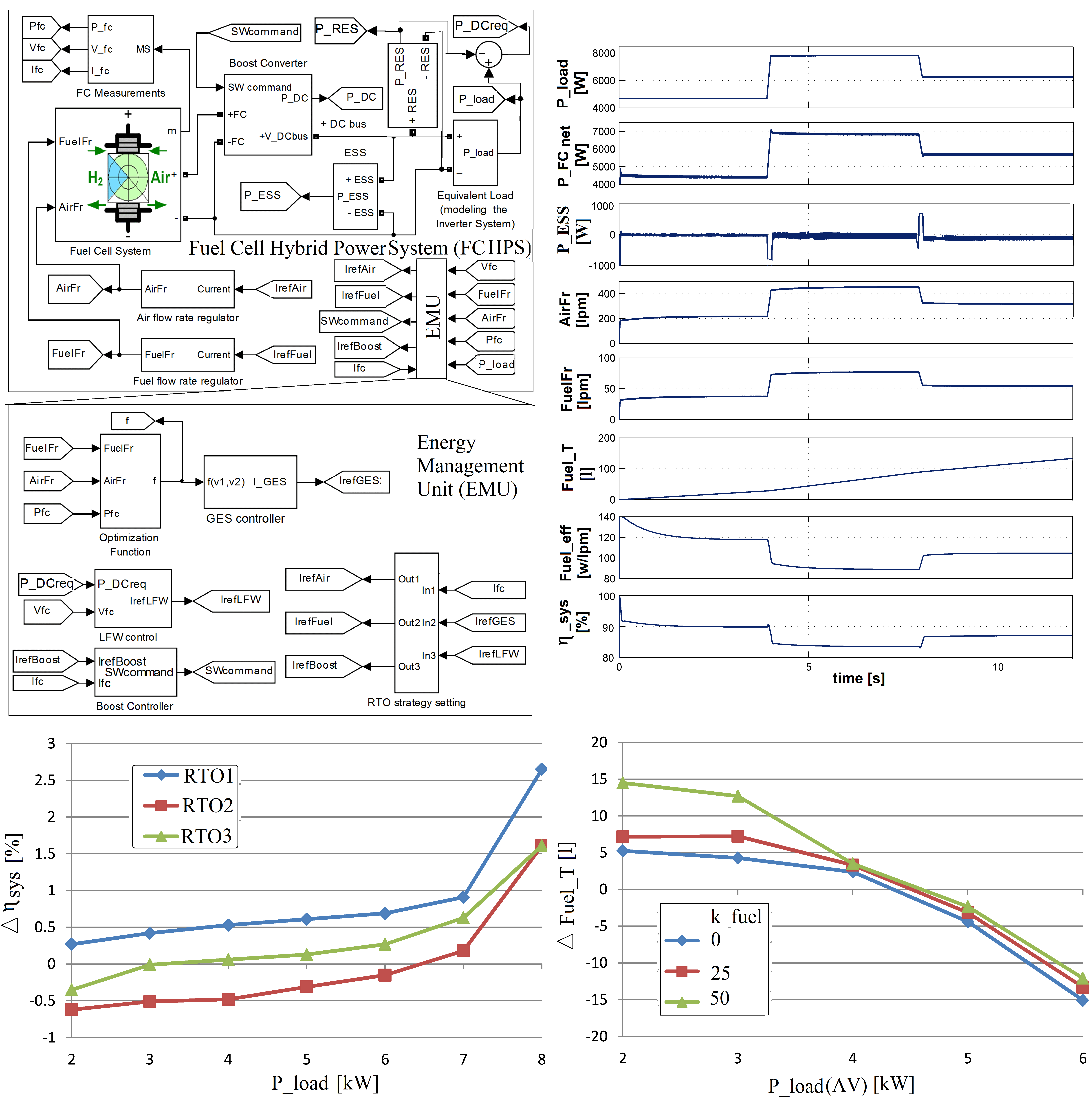
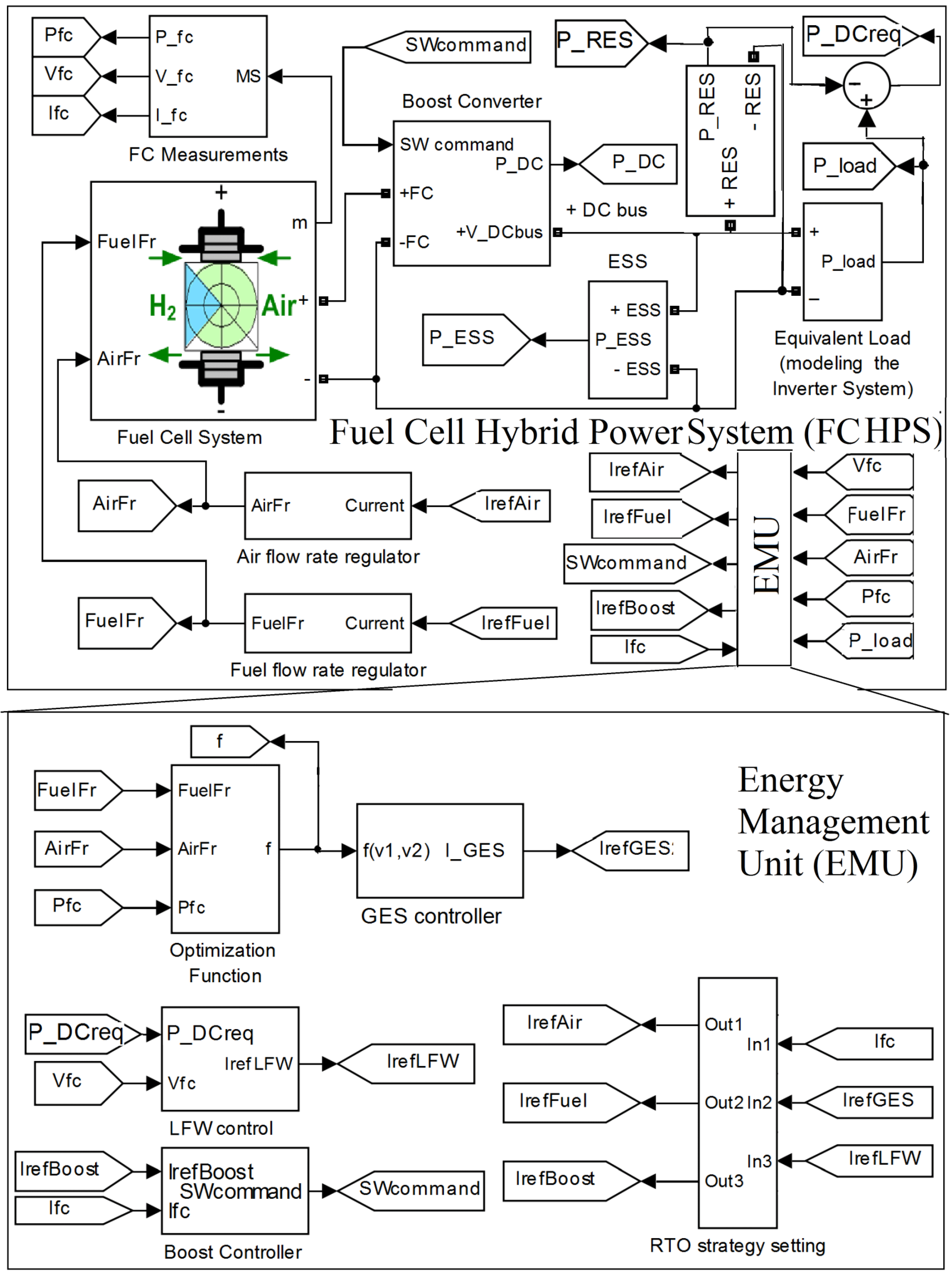
The FC-HPS based on Renewable Energy Sources (RES block in Figure 3—top) and the EMU (Figure 3—bottom) are presented in Figure 3. The output of the LFW controller, Iref(LFW), will be estimated based on power flow balance on DC bus (8):
CDCudcdudc/dt = pDC + pESSpDCreq
where the capacitor CDC filters the voltage on DC bus (udc). The p D C ,   p E S S   a n d   p D C r e q , represent the output power of the boost converter, the power of Energy Storage System (ESS), respectively the power required from the FC system, on DC bus, via the boost converter:
pDCreq = pLoadpRES
The output power of the FC boost converter is:
pDC = ηboostpFCnet
where ηboost ≅ 95% represents the efficiency of the boost converter.
Thus, the average value (AV) of the power flow balance (8) will be given by (11):
0 = ηboost PFCnet(AV)+ PESS(AV)PDCreq(AV)
When the battery works in mode “charge-sustaining”:
PESS(AV) ≅ 0
then LFW reference will be given by (13):
Iref(LFW)IFC(AV) = PDCreq(AV)/(VFCnet(AV) ηboost)
where the power requested on DC bus is the load demand from DC loads and AC loads via the inverter systems minus the available RES power:
pDCpDCreq = pLoadpRESPDCreq(AV)PLoad(AV)PRES(AV)
The inputs of the boost controller (Iref(boost)), the air regulator (Iref(Air)), and the fuel regulator (
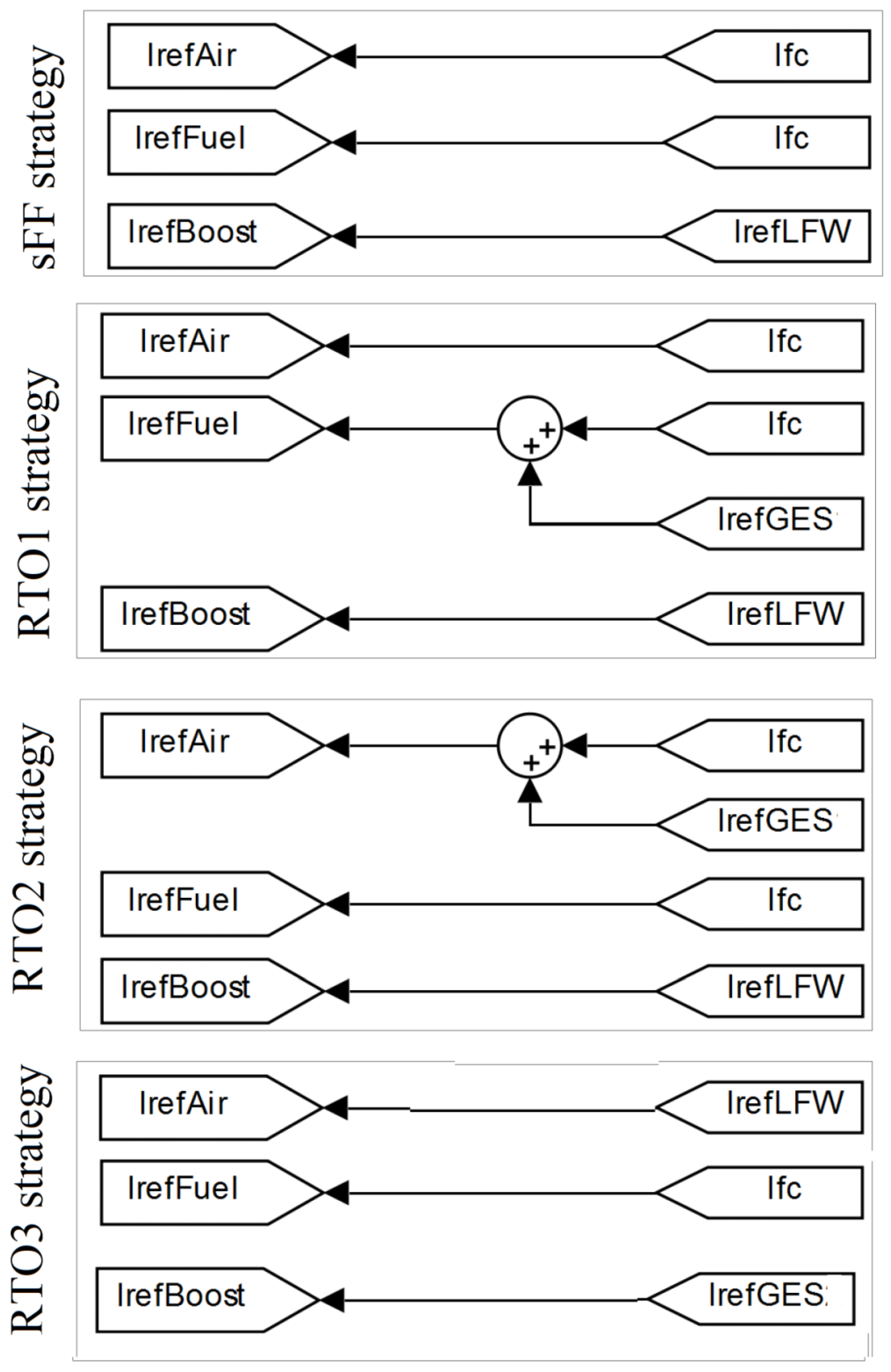
Iref(Fuel)) will be controlled by the GES references based on RTO strategies setting (see Figure 4 and Table 1), as follows: the RTO1 strategy uses Iref(boost) = Iref(LFW)., Iref(Fuel) = IrefGES + IFC and Iref(Air) = IFC, the RTO2 strategy uses Iref(boost) = Iref(LFW)., Iref(Air) = IrefGES2 + IFC and Iref(Fuel) = IFC (both strategies being tested in [97,98] for the FC-HPS without support from the RES), and the RTO3 strategy uses Iref(boost) = IrefGES, Iref(Fuel) = IFC and Iref(Air) = Iref(LFW) (being tested in [84,99] for the FC-HPS without support from the RES).
The FC current will follow Iref(LFW) for the RTO1 and RTO2 strategies due to hysteretic control of the boost converter:
IFC(AV)PDCreq(AV)/(VFCnet(AV) ηboost)
Consequently, the FC net power generated will be given by (16):
PFC(AV) = IFC(AV)VFCnet(AV)PDCreq(AV)/ηboost
Thus, considering (12), PESS(AV) ≅ 0, the LFW control is implemented using (13). The smooth value of the load demand and the FC voltage can be obtained using the AV techniques or other filtering techniques as well [100,101]. So, a smooth value will be obtained for the reference Iref(LFW) and the FC system will be safe operated even under sharp dynamic profiles of the load demand and RES power.
The references Iref(Fuel) and Iref(Air) will define the inputs FuelFr and AirFr of the FC system based on the fueling regulators (17) [56]:
F u e l F r = 60000 R ( 273 + θ ) N C I r e f ( F u e l ) 2 F ( 101325 P f ( H 2 ) ) ( U f ( H 2 ) / 100 ) ( x H 2 / 100 )
A i r F r = 60000 R ( 273 + θ ) N C I r e f ( A i r ) 4 F ( 101325 P f ( O 2 ) ) ( U f ( O 2 ) / 100 ) ( y O 2 / 100 )
where R and F the constants 8.3145 J/(mol K) and 96485 As/mol, and the parameters (NC, θ, Uf(H2), Uf(O2), Pf(H2), Pf(O2), xH2, yO2 ) are defined in [56].
The air and fuel regulators use 100 A/s slope limiters for safe operation of the FC-HPS [102].
Note that due to LFW control of the FC system via the boost controller, the batteries will operate in charge sustaining mode for all RTO strategies analyzed in this paper. The advantages are related to battery size, its lifetime and maintenance cost, and simple implementation of the EMU (the constraints (3c) for the battery SOC are clearly respected).
The sFF strategy proposed in [56] will be used as reference with the LFW control implemented in the same manner (see Table 1) for a fair comparison of each strategy RTOk, k = 1 ÷ 7, based on the gaps (18) in the performance indicators:
Δηsys = ηsyskηsys0
ΔFueleff = FueleffkFueleff0
ΔFuelT = FuelTkFuelT0
A PEMFC Matlab Simulink model with parameters: 6 kW/45 V is used in this study. For this model, the constant time is put to 0.1 s value. The variable voltage of FC (VFC) is raised to 200 V by using a boost converter V D C V D C ( r e f ) = 200   V . The control type used for the boost converter is of hysteretic type with 0.1 A hysteresis band.
Similar to [103], to mitigate the pulses on the DC bus a ESS semi-active topology is chosen. This topology has a battery stack connected on DC bus (lithium-ion batteries with 100 Ah/100 V) and an ultracapacitors’ stack with nominal capacity of 100 F. For this ultracapacitors’ stack we have the following typical values: ESR—the equivalent series resistor—the value is 0.1 Ω, EPR—the parallel resistor—the value is 10 kΩ, and the initial voltage are set on 100 V, so to connect the ultracapacitors’ stack to the DC bus, is used a bidirectional DC-DC converter. For all other model parameters, the values are the set by default. Also, the initial battery stack SOC is 80%. Both stacks use models from Matlab and Simulink® (R2013a, MathWorks, Natick, MA, USA) toolboxes (with the outputs that are offered by each model, such as SOC signal for the battery’s model, and which all are explained in the help page). Furthermore, to filter the voltage on DC bus, a capacitor, C D C , with 100 μF is used (the initial value of VDC = 200 V) [103].

4. Results

The GES-based RTO strategies will search the optimum of the optimization function (3a) for three sets of the k n e t   and   k f u e l values (weighting coefficients): in the first situation, A, we have the following values for coefficients: knet = 0.5, kfuel = 0), for the second situation, B, we have the following values for coefficients: knet = 0.5, kfuel = 25, and for the third situation, C, the values for coefficients are: knet = 0.5, kfuel = 50. Different scenarios were performed in this analysis. These scenarios have taken into account the power flow over the DC bus: the load demand has been both, variable and constant, also having or not having the power of RES.

4.1. HPS under Constant Load Demand and kfuel = 0 and PRES = 0

The value of the performance indicators ηsys0, Fueleff0, and FuelT0 for the sFF strategy are presented in [71].

FC Electrical Efficiency

Results such as deficiencies in fuel economy, fuel efficiency, and global fuel efficiency are presented in Table 2, Table 3 and Table 4 for each strategy RTOk, k = 1 ÷ 3, compared to sFF strategy in case A (kfuel = 0) under constant load.
The fuel economy are presented in Table 5, Table 6 and Table 7 for each strategy RTOk, k = 1 ÷ 3, compared to sFF strategy in case A (kfuel = 0), B (kfuel = 25), and C (kfuel = 50) under constant load.
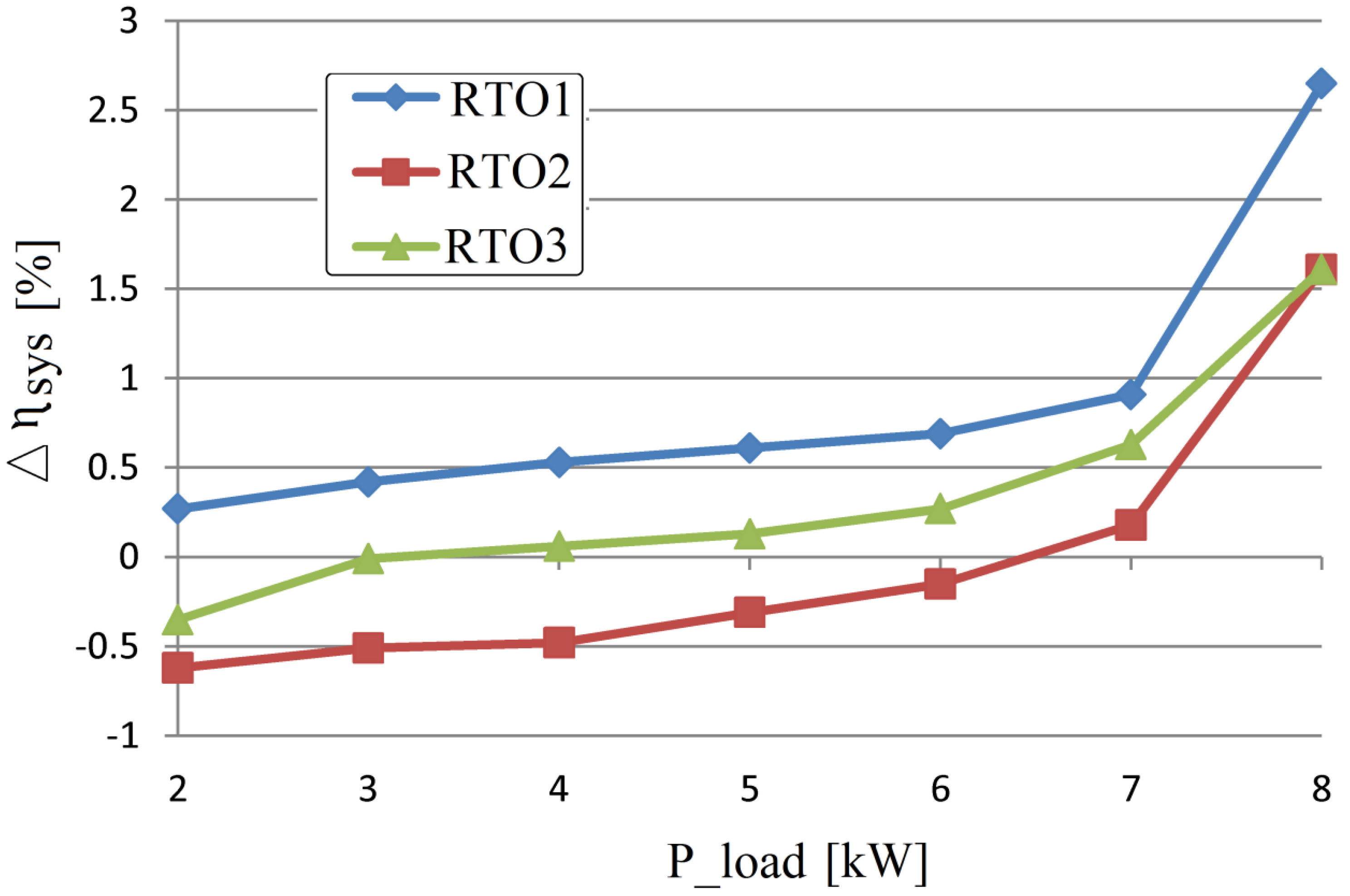
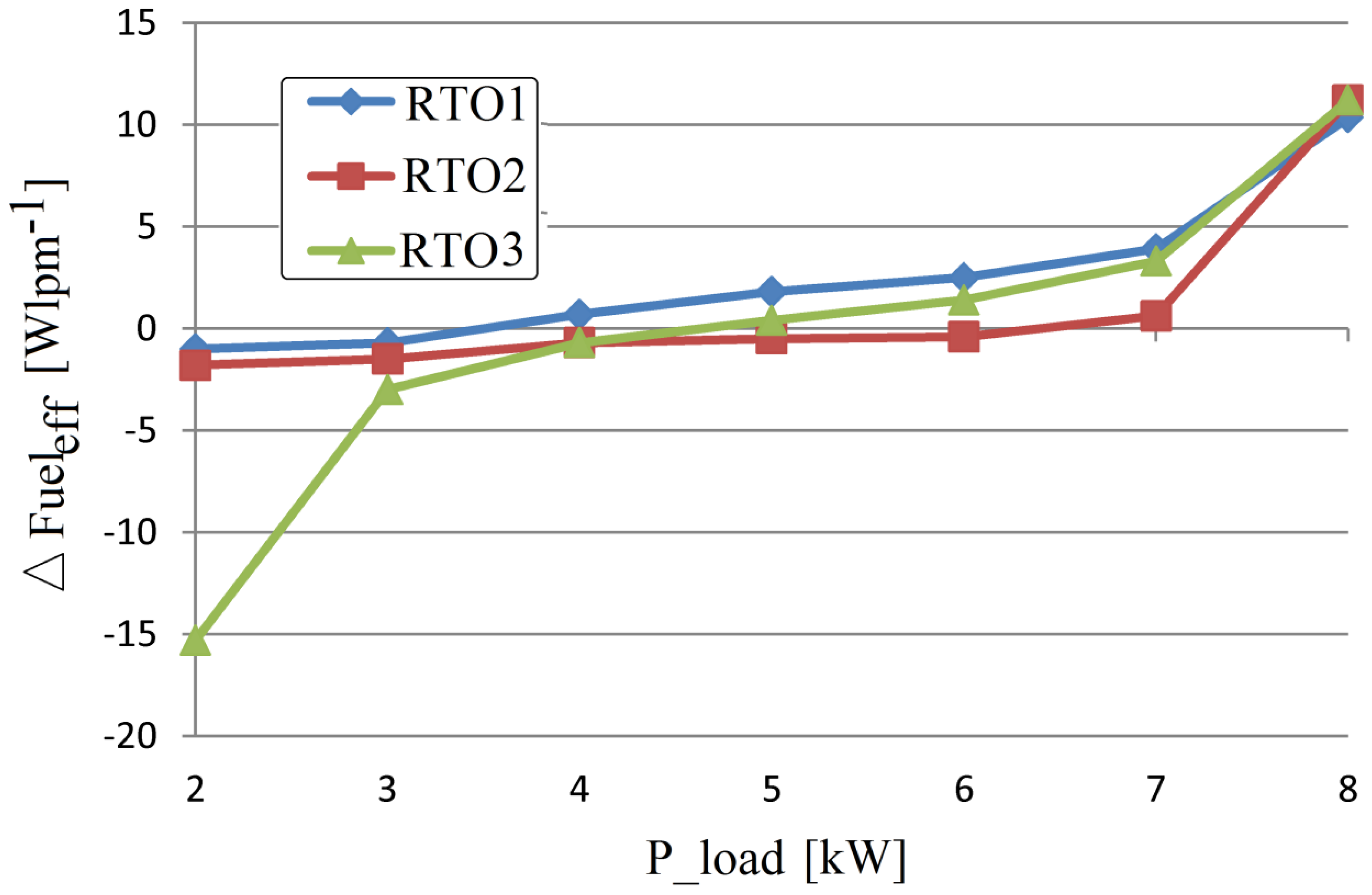
For the RTO1, RTO2 and RTO3 strategies, the deficiencies of the FC electrical efficiency and for the fuel efficiency are shown in Figure 5 and Figure 6. Fuel economy for the RTO1, RTO2, and RTO3 strategies in case A ( k f u e l = 0 ), B ( k f u e l = 25 ), and C ( k f u e l = 50 ) under constant load is shown in Figure 7, Figure 8 and Figure 9.
The gaps in FC electric efficiency is positive in full range of the load demand for the RTO1 strategy and best compared to strategies RTO2 and RTO3 (see Figure 5). Also, the fuel efficiency for RTO1 strategy is better compared to strategies RTO2 and RTO3 (see Figure 6). Fuel economy for the strategies RTO1 and RTO2 has almost the same shapes of evolution with load demand. Almost the same values for light load, but different values for high load are obtained (see Figure 7 and Figure 8). So, the FC net power could be maximized if the FC vehicle ascends up a hill using any of the RTO strategies outlined in this paper. Also, remember that the best fuel economy result for case B ( k f u e l = 25 ), so the fuel economy could be maximized if the FC vehicle ascends up a hill by choosing the appropriate value for weighting parameter kfuel. The performance of the RTO strategies outlined in this paper must be validated in different scenarios below.

4.2. Fuel Economy for the HPS under Variable Load Demand, PRES = 0, and Different kfuel

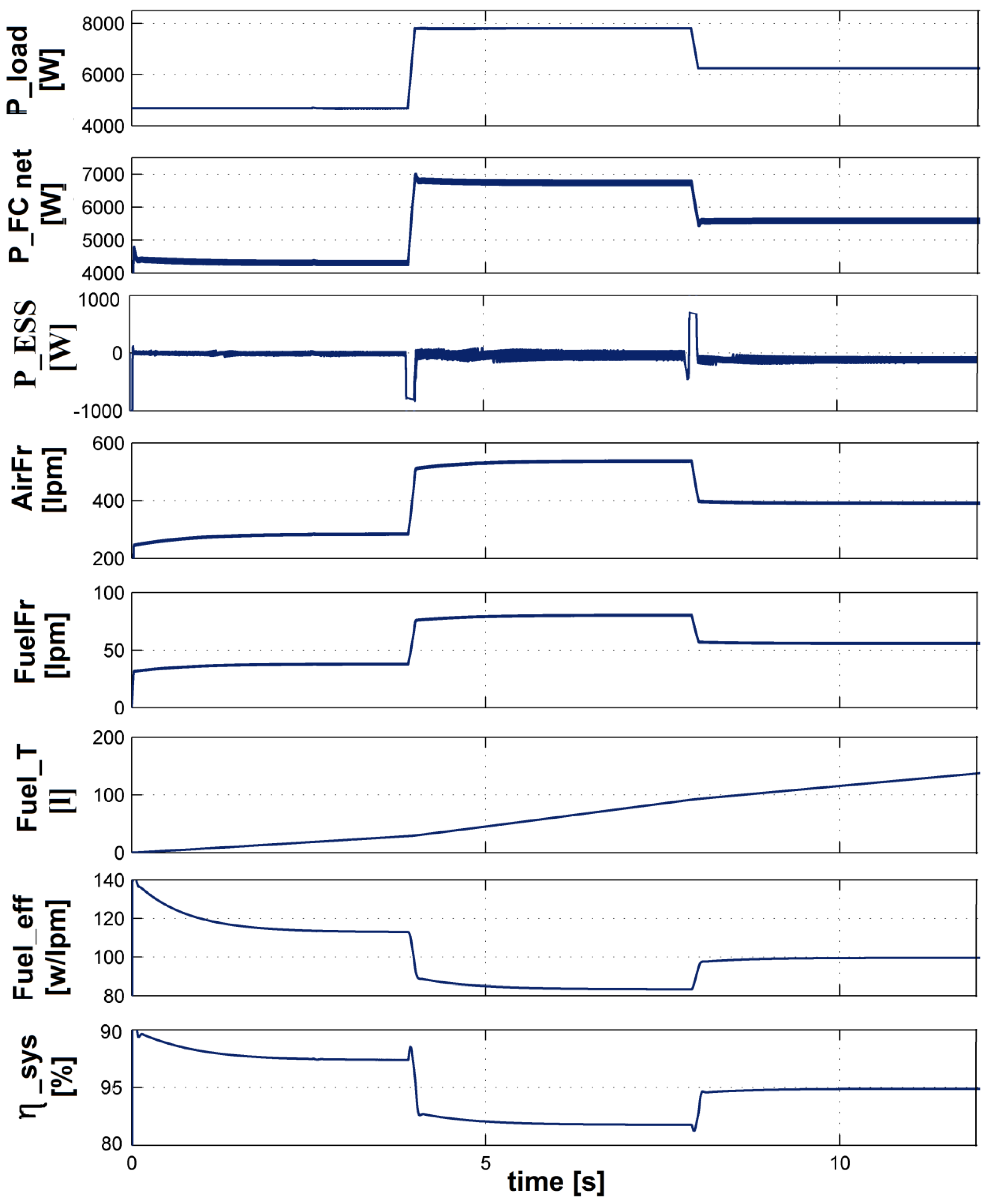
Only to exemplify that the LFW control of the boost converter operates based on (13), the behavior of the FC-HPS under 6.25 kW LC for the strategies RTO1 (Iref(LFW) = Iref(boost), Iref(Fuel) = IrefGES2 + IFC and Iref(Air) = IFC) with kfuel = 25 is presented in Figure 10.
The load cycles of 6.25 kW average power (Pload(AV) = 6.25 kW) is presented in first plot of Figure 10, but other load cycles that are used in this study as well, with different Pload(AV) values mentioned in Table 8, are defined in [71]. The fuel economy F u e l T O ( L C ) for the sFF strategy is presented as reference in Table 8.
The structure of the Figure 10 is as follows: the first plot shows the variable profile of the load power (PLoad); the second plot shows the generated FC net power profile (PFCnet) and this follows the load demand, highlighting that the LFW control operates properly; the third plot shows the ESS power, highlighting the advantage of LFW control implementing: the battery operating mode will only be of the charge-sustaining type ( P E S S ( A V ) 0 ), the DC bus power flow balance being sustained only during sharp variation of the load demand; the next two plots show the fueling flow rates (AirFr and FuelFr); the last three plots show the fuel consumption (FuelT), the fuel efficiency (ΔFueleff), and the FC electric efficiency (
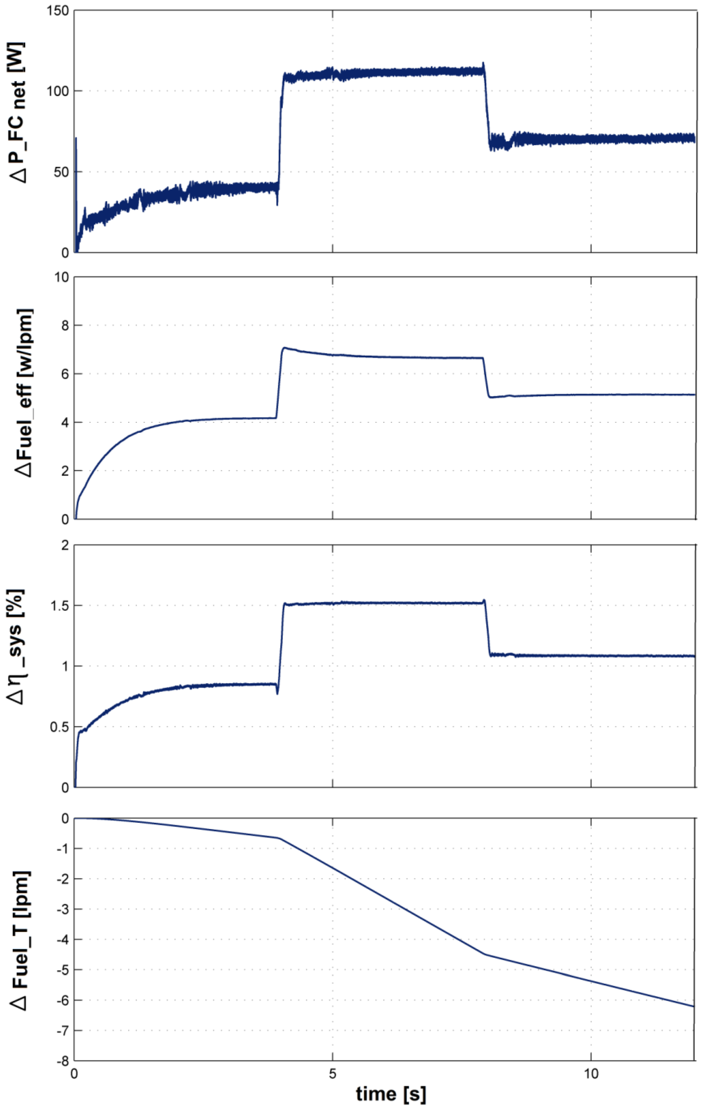
ηsys). It is worth to mention that the shape of the signals for the strategies RTO1, RTO2, and RTO3 will look almost the same, but small differences in performance indicators can be observed for different LCs (which are mentioned in Table 9 for each RTO strategy). For example, the differences in FC net power (ΔPFCnet = PFCnetkPFCnet0, k = 1, 2, 3), FC energy efficiency (Δηsys = ηsyskηsys0), fuel efficiency (ΔFueleffFueleffkFueleff0), and fuel economy (ΔFuelTFuelTkFuelT0) are represented in Figure 11 for RTO1 strategy with kfuel = 25 (the value where the best fuel economy was obtained for constant load).
The fuel economy for strategies RTO1 is of 6.36 liters (see also Table 10) and this performance indicator will be used to compare selected RTO strategies under variable load. The fuel economy is presented in Table 9, Table 10 and Table 11 for selected RTO strategies compared to sFF strategy.
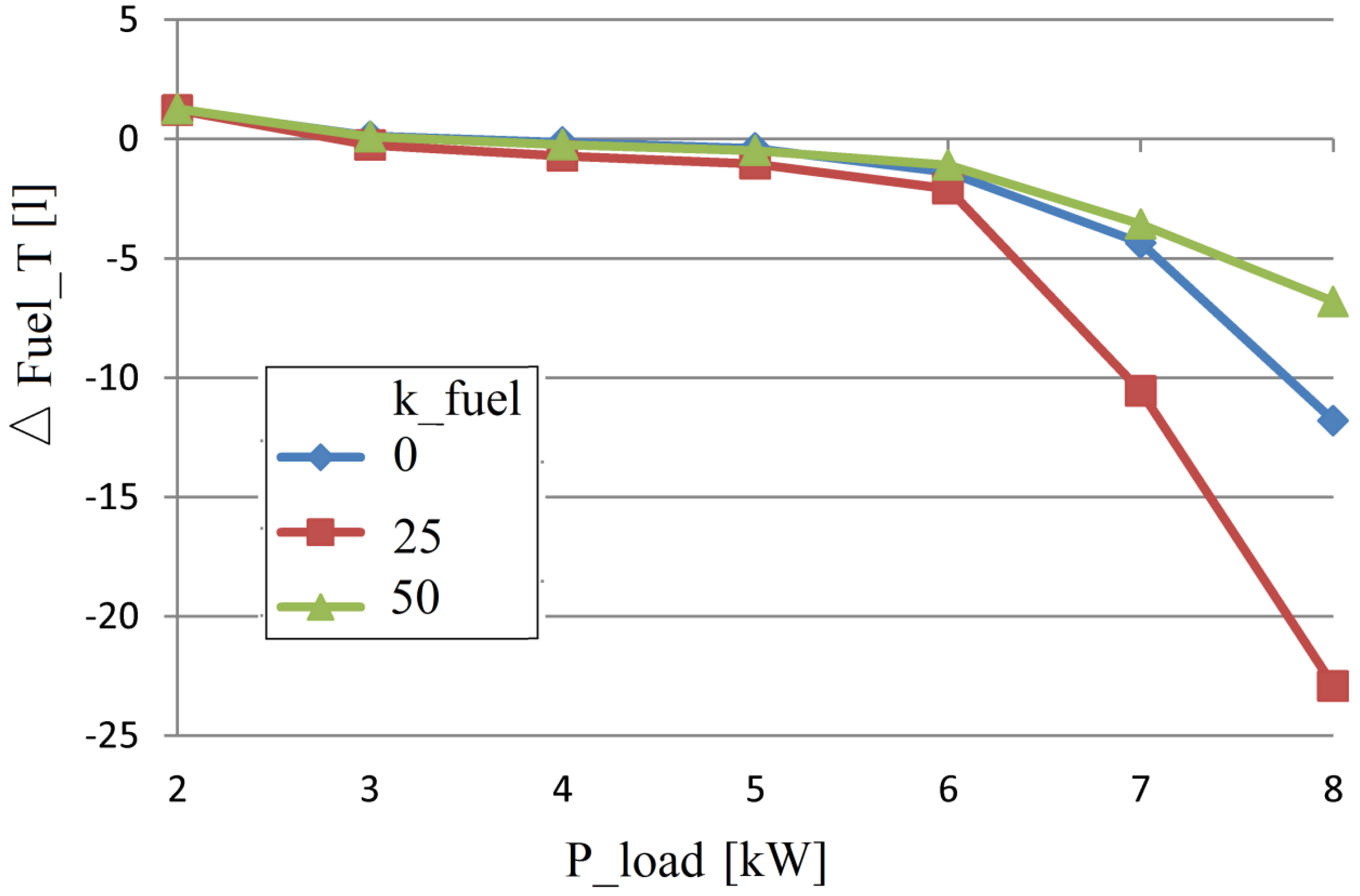
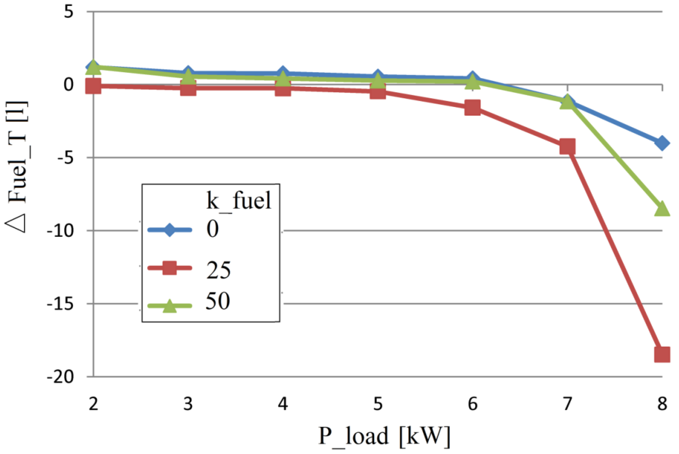
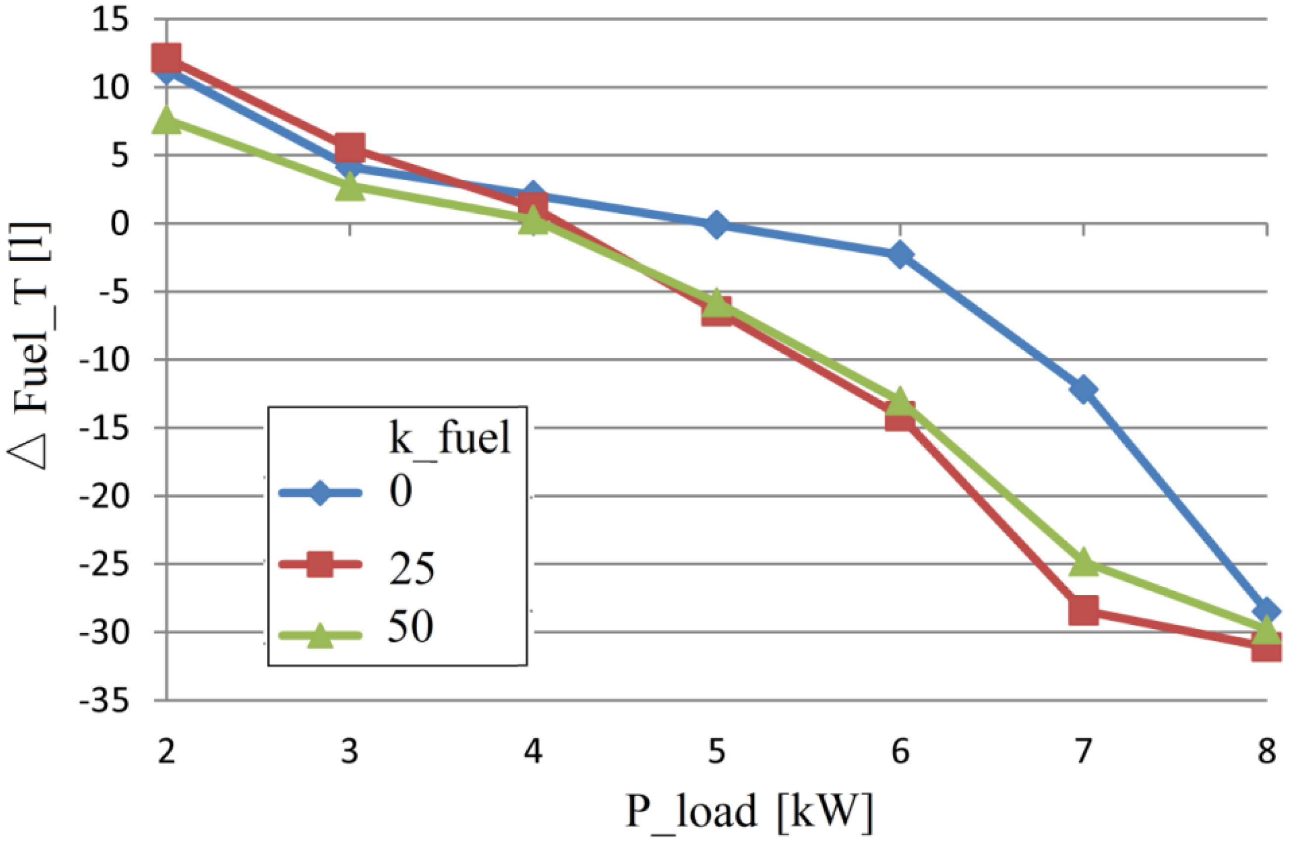
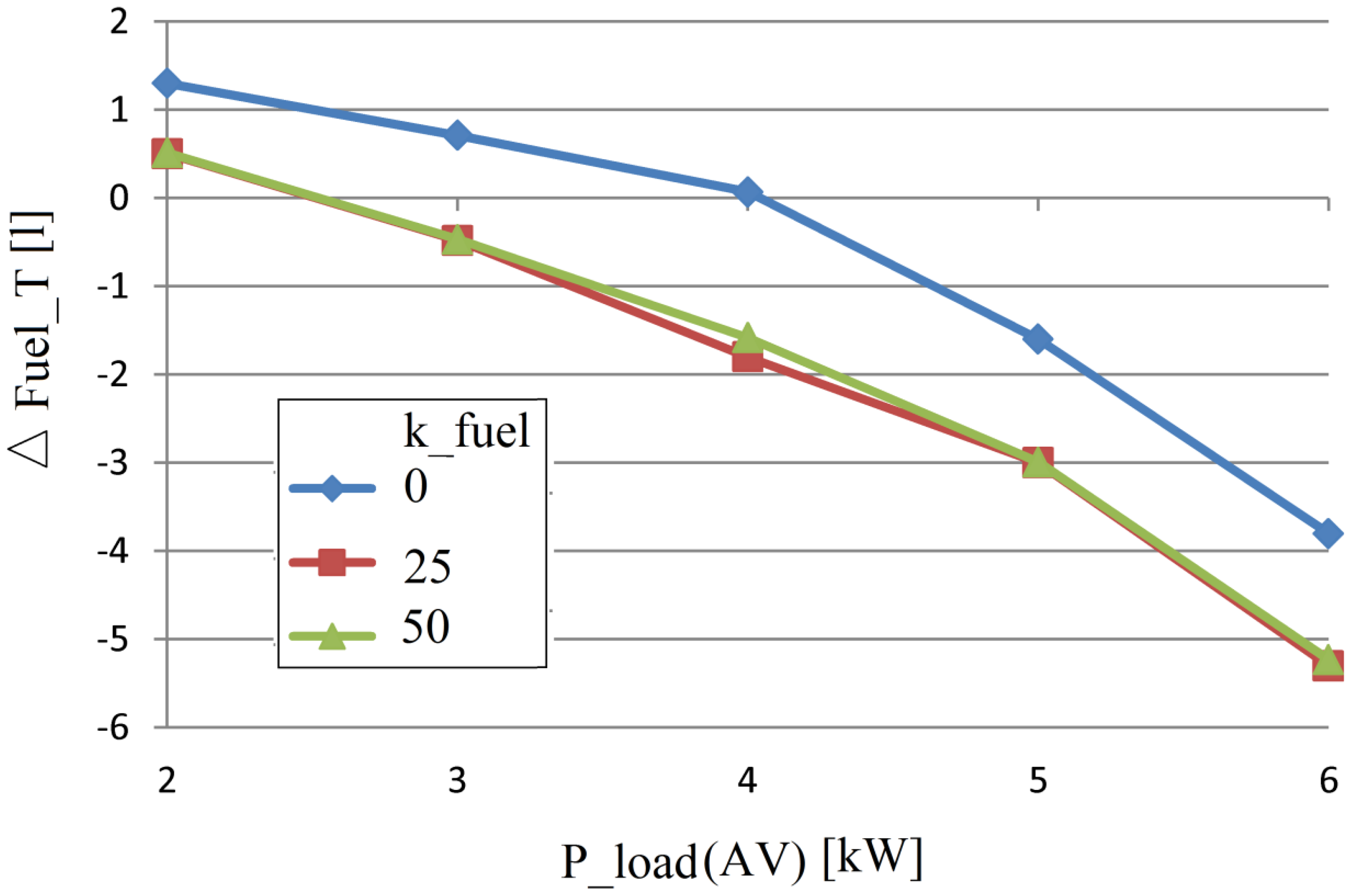
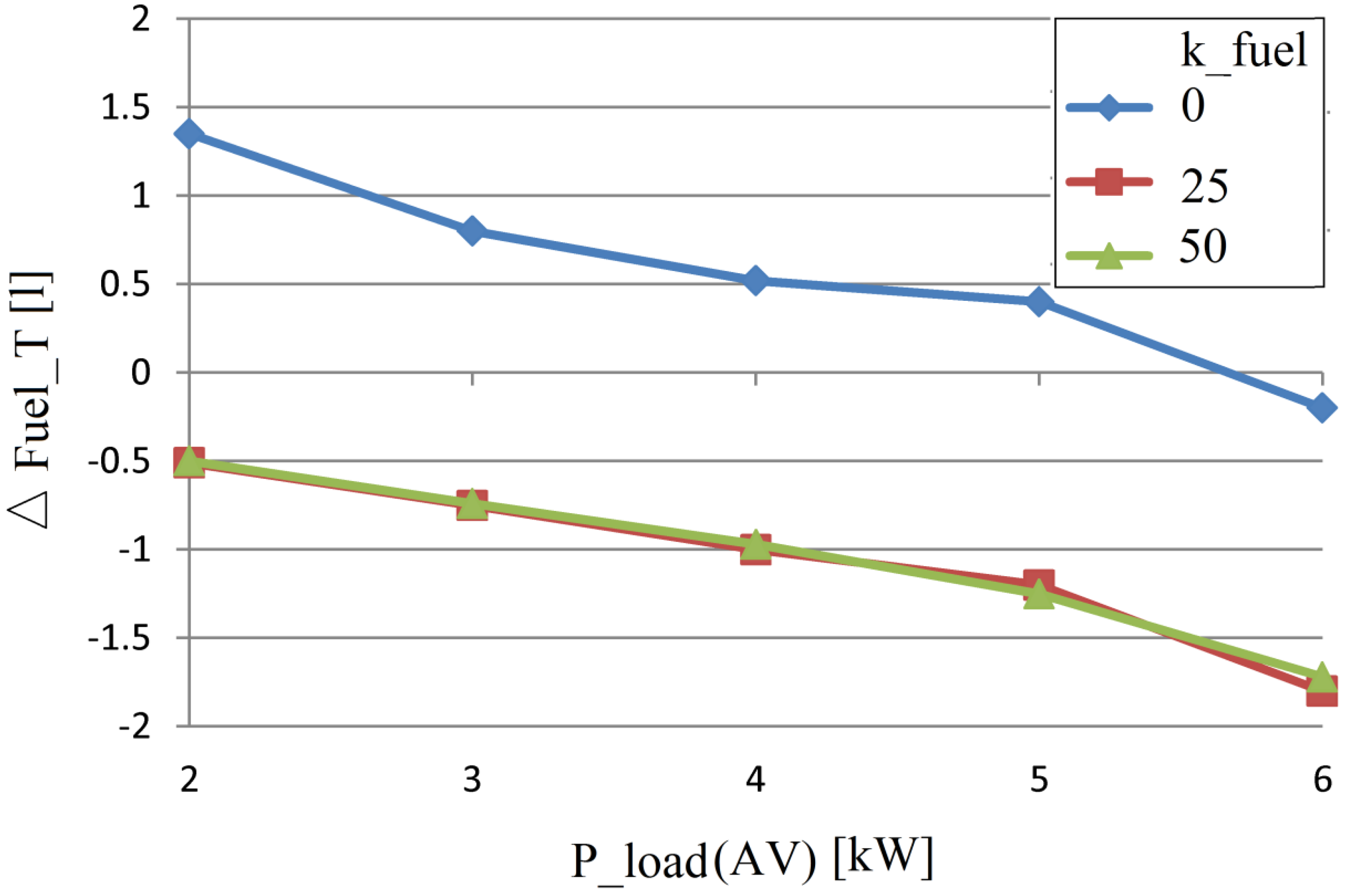
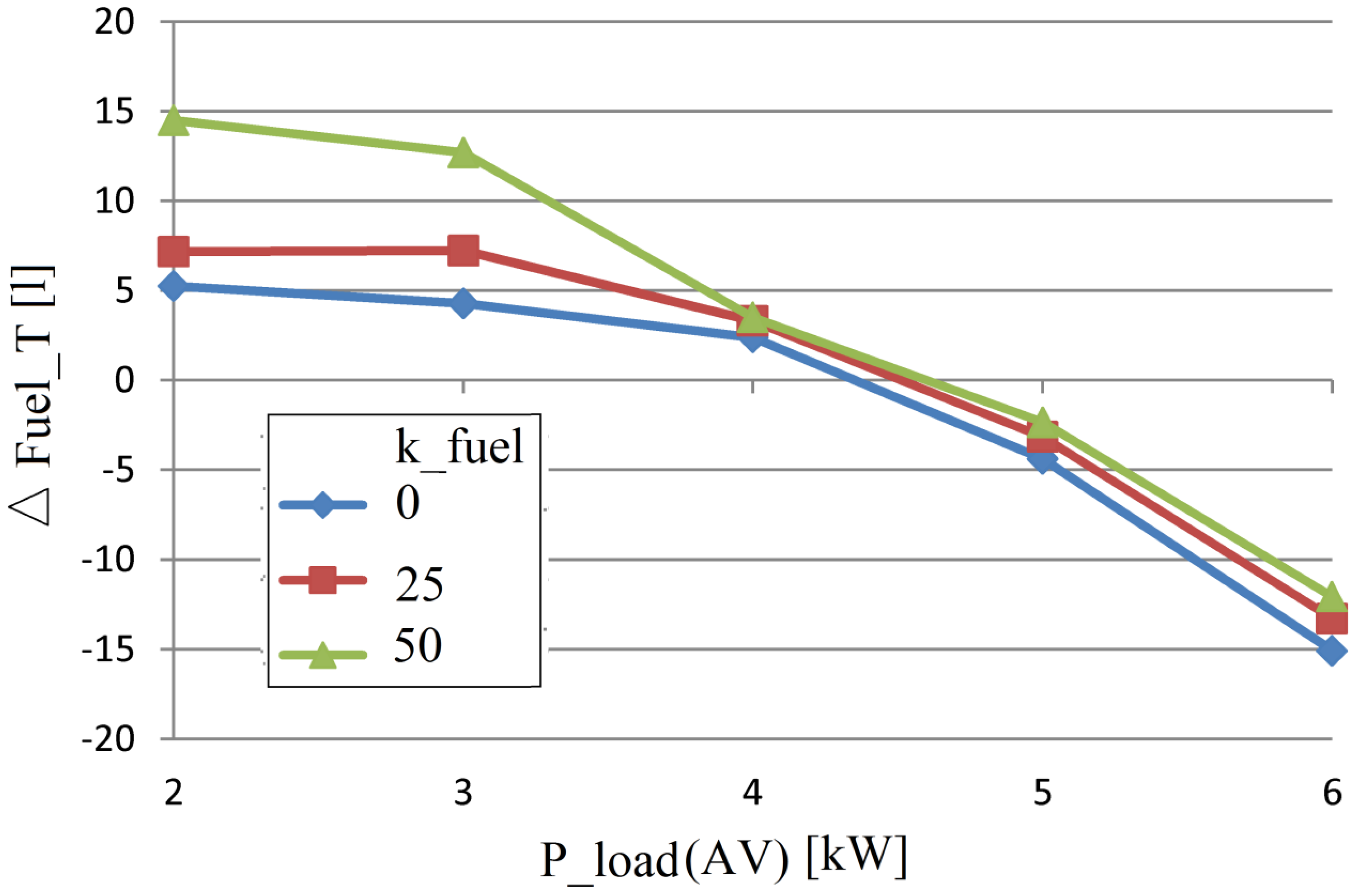
The fuel economy for selected RTO strategy, in the all situation, A ( k n e t = 0.5 , k f u e l = 0 ), B (( k n e t = 0.5 , k f u e l = 25 ), and C (( k n e t = 0.5 , k f u e l = 50 ), under variable load demand is shown in Figure 12, Figure 13 and Figure 14.
Note that the values for the fuel economy increases for some strategies, RTO1 and RTO2, only if kfuel ≠ 0. A sensitivity analysis was performed considering the parameter k f u e l with values between 10 and 50, for understand the shape of the optimization function in this variable k f u e l .
The results show that the optimization function is multimodal, with parameter kfuel, so any value for k f u e l , between 10 and 50, can be used and the same fuel economy can be obtained for two different values of k f u e l . It is worth mentioning that any value of k f u e l in the range of values between 10 and 50 will improves the fuel economy for the strategies RTO1, in almost the full range of load demand and this is higher than that obtained with the RTO3 strategy, but no improvement in fuel economy at light load is obtained for RTO3 strategy if kfuel ≠ 0. Also, it worth to mention the the fuel economy is almost the same for kfuel = 0 or kfuel ≠ 0 compared to sFF strategy for P l o a d ( A V ) > 5   kW (as it can be observed at constant load as well; see Figure 9), but clearly higher than that obtained with the booth strategies RTO1 respectively RTO2.
Consequently, the rules of the RTO switching strategy for best fuel economy of 6 kW FC-HPS could be defined as follows: (i) set the weighting coefficient kfuel to optimum value (around of 25); (ii) if the load demand is lower than 5 kW then the recommended strategy must be the RTO1 strategy; (iii) if the load demand is higher than 5 kW then the recommended strategy must be the RTO3 strategy.

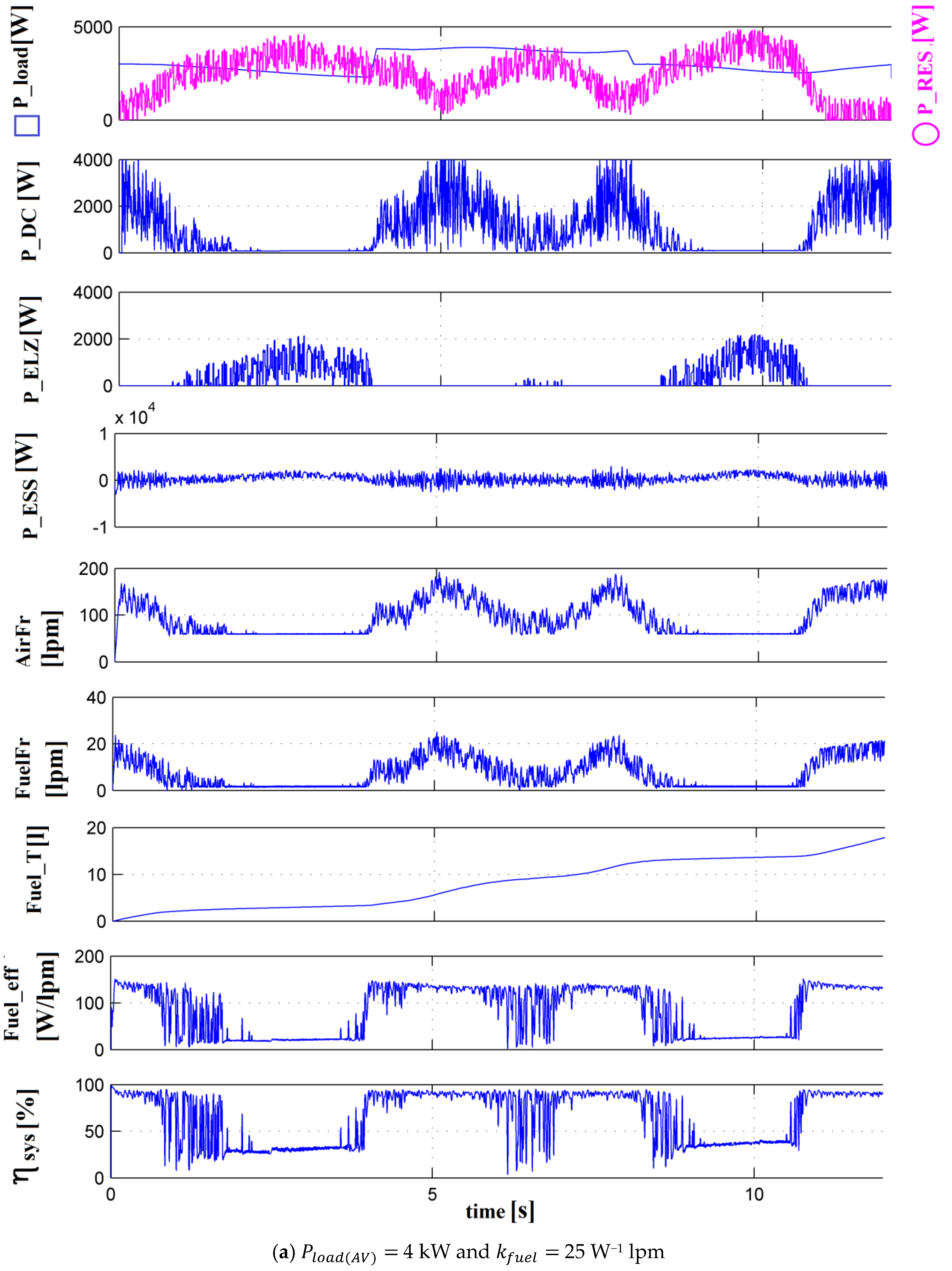
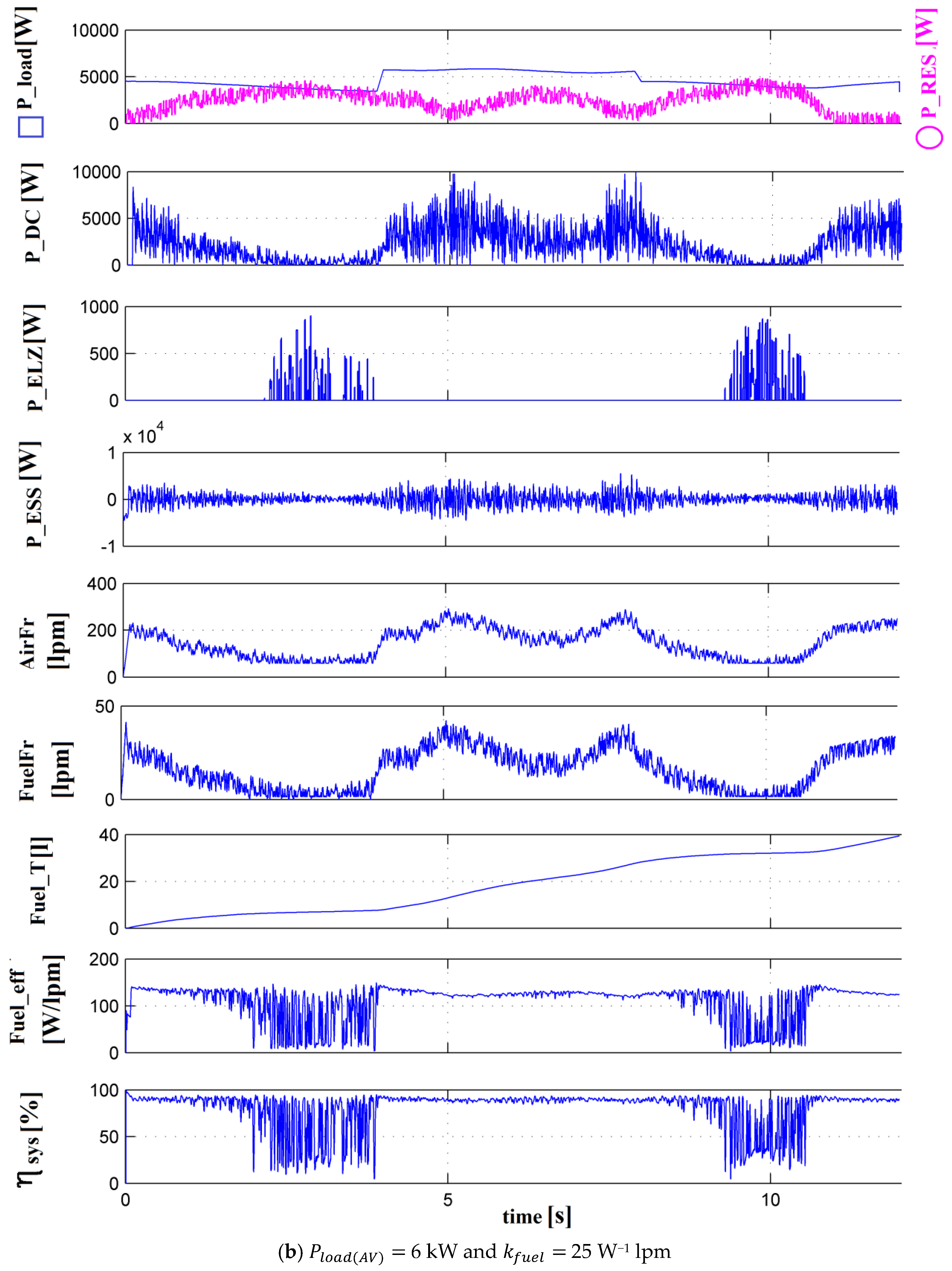
4.3. Fuel Economy for the HPS under Variable Load Demand and PRES ≠ 0

For exemplify, in Figure 15 is presented the functioning for the RTO3-based FC-HPS under variable load and RES power for two AV levels of the load demand ( P l o a d ( A V ) = 4 kW and P l o a d ( A V ) = 6 kW in Figure 15a,b). The plots’ organization presented in Figure 15 is: the first plot shows the profile of the load power. The second plot shows the FC net power profile. This FC net power follows the load demand due to the implemented LF control. The third plot shows the Energy Storage System power, highlighting the LF control advantage: the ESS operate in the charge sustaining manner ( P E S S ( A V ) 0 ); the fueling flow rates (AirFr and FuelFr) are presented in the next two plots, and, in the last three plots, the fuel consumption, the fuel efficiency, and the FC energy efficiency are presented.
If the RES power is higher than the load demand ( P R E S > P l o a d ), the fuel cell operate in standby mode, at low power. This is done by limiting fueling flows, avoiding a more complicated star-stop procedure.
The resulting power excess, ( P R E S P l o a d ) must be used (one use it to supply an electrolyzer). If this power excess is not used, it is necessary to monitor the charging state of the battery, in order to avoid full charging.

5. Discussion

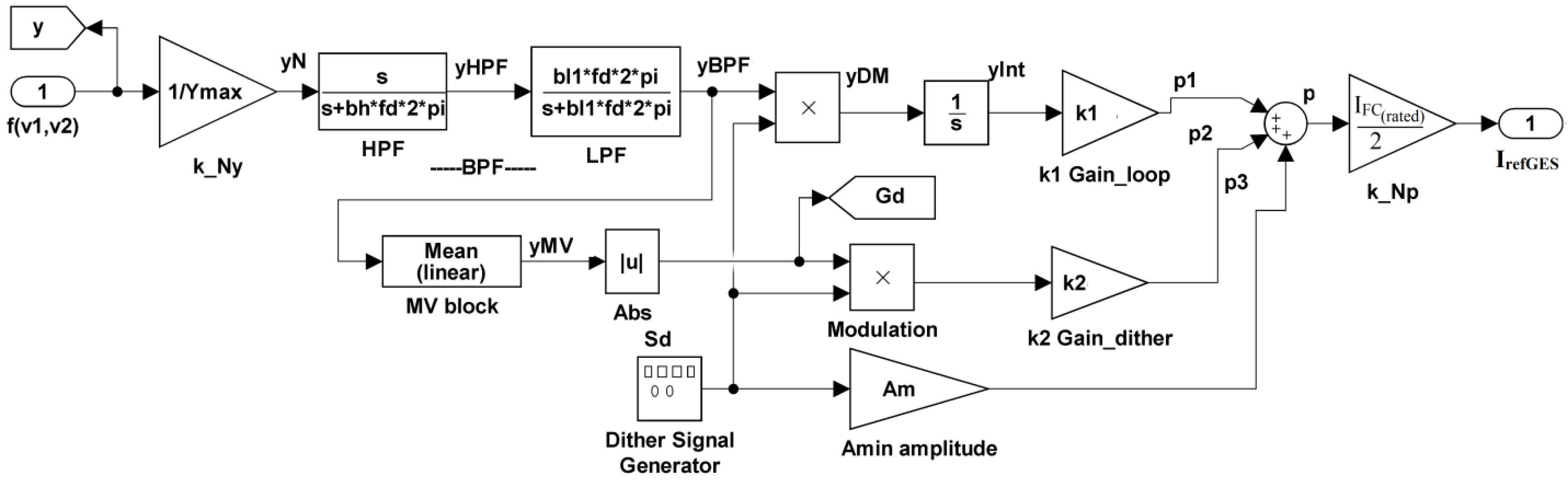
Differently from the sFF strategy, to explain the fuel economy obtained with the GTO-based RTO strategy, it is necessary follow the values of the performance indicators mentioned above and the values for the adjustment parameters and the gains. Taking into account design rules from [75], tuning parameters k 1 , respectively k 2 , were designed for fuel cell system with 6 kW power.
Normalization gains must to accommodate the booth values: yN respectively p for the full range of searching. In this case, the following values were used in the simulation: k N y = 2 Y M a x 1 3000 and k N p = I F C ( r a t e d ) 2 60 . The following values for weighting coefficients k n e t = 0.5 W 1 lmp, respectively k f u e l = 25 W 1 lpm were chosen to give an approximately identical contribution to FC net power ( k n e t · P F C n e t 3000 ) , and for the fuel consumption efficiency ( k f u e l · F u e l e f f 25 · 110 = 2750 ) into the optimization function ( Y M a x = f 5750 ) . The load demand varies in range of 2 kW to 8 kW and the FC current from 10 A to 240 A. Thus, considering these values, the optimization function varies from about 4400 to 6400. Thus, the signal y N varies from 1.5 ( 4400 3000 ) to 2.1 ( 6400 3000 ) and the signal p from 1 6   ( 10 60 ) to 4 ( 240 30 ) . The adaptive characteristic of the GES control has 100% ability to discover the global optimum for these variations in the parameters [76,96].
Since the imposed objective is to improve the fuel cell net power, and not to save the fuel (the form of optimization function is f = k n e t · P F C n e t ), we will get more fuel economy by using the sFF strategy, in comparison with RTO strategies if k n e t = 0 and the load is lower ( P l o a d <   3 k W ) .
If the Pload < 3 kW, the results obtained are very little different when performing a sensitivity analysis in according with: k f u e l 0 . This is possible because we have low values for search resolution (RS), which become lower than 0.5% and hit count decreases (so a suboptimal value was found instead of the optimum).
Except for the RTO3’s strategy al light load (Pload(AV) < 4 kW for kfuel ≠ 0), in all other cases, we achieve fuel economy, both for constant load and for variable load. The exception occurs when RS < 0.5% at light load, but note, compared to strategies RTO1 and RTO2, the high fuel economy of RTO3 strategy that is obtained for Pload(AV) > 4 kW due to optimal control of the boost converter.
The multimodal characteristic of the optimization function in variable kfuel resulted after the sensitivity analysis performed for different kfuel values, in the 10–50 range. In this way, for any kfuel value in the above mentioned range, the fuel economy can be improved.
Several factors influence tracking efficiency. These factors are: the dynamics of the load; the RES power profile; and last but not least, the tracking time (the response time of the search loop) [25,26,27,28,29].
As was mentioned, if we have a 100 Hz sinusoidal dither, 10 periods of dither (0.1 s) represent the tracking time for the GES control. Consequently, the dynamic phenomena such as the RES power fluctuation and high and sharp dynamics of load demand will influence the performance of any RTO strategy (including the sFF strategy) if the tracking time is not lower that time constants of the process under optimization. For the stationary tracking accuracy parameter, the following results are obtained: for stationary mode, and for the dither frequencies ranging from 10 Hz to 1000 Hz, we have an accuracy of 99.99%. If we have load pulses mode, and we have 100 Hz for the dither frequency, we obtain a tracking accuracy of 99.86%. This accuracy decreases to 98% if the dither frequency is 1000 Hz [78]. Taking into account the sensitivity analysis performed for the dither signal frequency in the interval between 10 Hz and 1000 Hz, the best results appear when we use a sinusoidal dither signal with a hundred Hz frequency.
For a fair comparison, the LFW reference Iref(LFW) was used as reference input for the boost controller (Iref(boost)) in the strategies RTO1 and RTO2, and for air regulator in RTO3 strategy. The inputs of the air regulator (Iref(Air)) and the fuel regulator (Iref(Fuel)) in the strategies RTO1 and RTO2 were controlled by the GES reference (IrefGES) and the FC current (IFC) to optimize the FC system operation as follows: the RTO1 strategy uses Iref(Fuel) = IrefGES + IFC and Iref(Air) = IFC, and the RTO2 strategy uses Iref(Air) = IrefGES + IFC and Iref(Fuel) = IFC. The RTO3 strategy uses Iref(boost) = IrefGES, Iref(Air) = Iref(LFW), sand Iref(Fuel) = IFC. Thus, the RTO3 strategy uses the boost convertor to optimize the FC system operation, which has response time much shorter than the fueling regulators and speed advantage in searching the optimum of the optimization function compared to strategies RTO1 and RTO2. Consequently, for best fuel economy, the potential rules of an advanced RTO switching can be defined as follows: (i) set the weighting coefficient kfuel ≠ 0 (in range 10 to 50); (ii) if the load demand is lower than 5 kW then the recommended strategy must be the RTO1 strategy; (iii) if the load demand is higher than 5 kW then the recommended strategy must be the RTO3 strategy.
The next work will be focused on a comparative analysis of the fuel economy obtained by using the RTO strategies proposed in this paper with those analyzed in [71].

6. Conclusions

In this paper, besides a brief presentation of current RTO strategies and a critical assessment of proposed Extremum Seeking (ES) algorithms, the fuel economy of three Renewable Fuel Cell Hybrid Power System (REW/FC-HPS) topologies has been analyzed.
In this paper, the dynamics on load demand and the electric power available from the Renewable Energy Sources (RESs), is proposed to be mitigated using the load-following (LFW) control in order to sustain the power flow balance on the DC bus within much power support from the battery. Because, in this case, the battery will work in charge-sustained mode, resulting clear advantages for FC vehicles related to battery size, its lifetime and maintenance cost.
The optimization objective can be set in real-time by changing the values of the weighting coefficients k n e t and k f u e k l in order to increase the overall fuel economy, the FC electrical efficiency, or other performance indicators defined for the HPS.
So, besides the proposal of the switching RTO strategy, the main results of this study can be summed up as follows:
  • In comparison with sFF strategy, the control strategies RTO1 and RTO2 offers a higher FC electric efficiency for all range of the load demand (see Figure 5).
  • The fuel efficiency of the strategies RTO1 and RTO3 is almost the same for Pload(AV) > 4 kW (see Figure 6).
  • The fuel economy of all RTO strategies analyzed here for kfuel= 0 is almost the same for Pload(AV) < 4 kW, but a three times higher fuel economy is achieved at maximum load considering the RTO3 strategy compared to RTO1 strategy (see Figure 7, Figure 8 and Figure 9 for kfuel = 0).
  • The fuel economy increases even further if kfuel ≠ 0 (see Figure 7, Figure 8 and Figure 9).
  • The conclusions about fuel economy for each RTO strategy remain the same for variable profiles of the load demand and RES power.
  • The variability of the RES power and load dynamics can be mitigated by the LFW proposed in this paper to sustain the power flow balance on the DC bus without much support from the batteries’ stack, which mainly operates in charge-sustained mode.
Finally, it worth to mention that exploration of space of the optimal solutions with two variables could have as result a higher fuel economy compared with one variable—based RTO strategies analyzed in this paper, but this assumption must further investigated.

Author Contributions

Conceptualization, Methodology, Validation, and Writing—Original Draft Preparation: B.N.; Writing—Review & Editing: O.M. and B.N.

Funding

This work was founded by two grants of the Ministry of National Education and Scientific Research, CNCS/CCCDI-UEFISCDI, within PNCDI III, code PN-III P1-1.2-PCCDI2017-0332 and title “Increasing the institutional capacity of bioeconomic research for the innovative exploitation of the indigenous vegetal resources in order to obtain horticultural products with high added value”, and within RDI Program for Space Technology and Advanced Research - STAR, code 167/2017 and title “Concept Development of an Energy Storage Unit Using High Temperature Superconducting Coil for Spacecraft Power Systems (SMESinSpace). The sponsors had no role in the design, execution, interpretation, or writing of the study. The research was performed in Research Center “Modeling and Simulation of the Systems and Processes”.

Conflicts of Interest

The authors declare no conflict of interest.

Nomenclature

AirFrAir Flow rate
AVAverage value
BPFBand-Pass Filter
fdDither frequency
DPDynamic Programming
ECMSEquivalent Consumption Minimization Strategy
EMSEnergy Management Strategy
EMUEnergy Management Unit
ESExtremum Seeking
aPESCAsymptotic Perturbed Extremum Seeking Control
PESCsScalar PESC
ESSEnergy Storage System
FuelFrFuel Flow rate
FCFuel cell
PFCFC stack power
PFCnetFC net power
PcmAir compressor power
ησψσFC electrical efficiency
effH2Hydrogen consumption efficiency
FC HPSFuel Cell Hybrid Power Systems
FuelFrFuel Flow rate
FuelTTotal Fuel Consumption
FueleffFuel Consumption Efficiency
FFTFast Fourier Transform
FESFlywheel energy storage
GESGlobal Extremum Seeking
GaPESCGlobal aPESC
HILSHardware-in-Loop System
HPFHigh-Pass Filter
HPSHybrid Power System
kNpOutput normalization gain
kNyInput normalization gain
LCLoad Cycle
LFWLoad-Following
MEPMaximum Efficiency Point
MPPMaximum Power Point
MVMean Value
MPCModel Predictive Control
MRACModel Reference Adaptive Control
PESCPerturbed Extremum Seeking Control
PMPPontryagin's Minimum Principle
PEMFCProton Exchange Membrane Fuel
PLoadStationary load power (constant power demand)
pLoadDynamic load power (variable power demand)
RTOReal-Time Optimization
RESRenewable Energies Source
SRSearching Resolution
sFFStatic Feed-Forward
SMESSuperconducting Magnetic Energy Storage
SOCState-Of-Charge
TaccTracking accuracy
WTWind Turbines

References

  1. Bizon, N.; Tabatabaei, N.M.; Blaabjerg, F.; Kurt, E. Energy Harvesting and Energy Efficiency: Technology, Methods and Applications; Springer: London, UK, 2017; Available online: http://www.springer.com/us/book/9783319498744 (accessed on 12 December 2018).
  2. Ijaodola, O.; Ogungbemi, E.; Khatib, F.N.; Wilberforce, T.; Ramadan, M.; Hassan, Z.E.; Thompson, J.; Olabi, A.G. Evaluating the Effect of Metal Bipolar Plate Coating on the Performance of Proton Exchange Membrane Fuel Cells. Energies 2018, 11, 3203. [Google Scholar] [CrossRef]
  3. Rafique, M.K.; Haider, Z.M.; Mehmood, K.K.; Zaman, M.S.U.; Irfan, M.; Khan, S.U.; Kim, C.-H. Optimal Scheduling of Hybrid Energy Resources for a Smart Home. Energies 2018, 11, 3201. [Google Scholar] [CrossRef]
  4. Sikkabut, S.; Mungporn, P.; Ekkaravarodome, C.; Bizon, N.; Tricoli, P.; Nahid-Mobarakeh, B.; Pierfederici, S.; Davat, B.; Thounthong, P. Control of High-Energy High-Power Densities Storage Devices by Li-ion Battery and Supercapacitor for Fuel Cell/Photovoltaic Hybrid Power Plant for Autonomous System Applications. IEEE Trans. Ind. Appl. 2017, 52, 4395–4407. [Google Scholar] [CrossRef]
  5. Ishaque, K.; Salam, Z. A review of maximum power point tracking techniques of PV system for uniform insolation and partial shading condition. Renew. Sustain. Energy Rev. 2013, 19, 475–488. [Google Scholar] [CrossRef]
  6. Liu, Z.-H.; Chen, J.-H.; Huang, J.-W. A review of maximum power point tracking techniques for use in partially shaded conditions. Renew. Sustain. Energy Rev. 2015, 41, 436–453. [Google Scholar] [CrossRef]
  7. Bizon, N.; Tabatabaei, N.M.; Shayeghi, H. Analysis, Control and Optimal Operations in Hybrid Power Systems—Advanced Techniques and Applications for Linear and Nonlinear Systems; Springer: London, UK, 2013. [Google Scholar]
  8. Olatomiwa, L.; Mekhilef, S.; Ismail, M.S.; Moghavvemi, M. Energy management strategies in hybrid renewable energy systems: A review. Renew. Sustain. Energy Rev. 2016, 62, 821–835. [Google Scholar] [CrossRef]
  9. Zhang, P.; Yan, F.; Du, C. A comprehensive analysis of energy management strategies for hybrid electric vehicles based on bibliometrics. Renew. Sustain. Energy Rev. 2015, 48, 88–104. [Google Scholar] [CrossRef]
  10. Peng, J.; He, H.; Xiong, R. Rule based energy management strategy for a series–parallel plug-in hybrid electric bus optimized by dynamic programming. Appl. Energy 2017, 185, 1633–1643. [Google Scholar] [CrossRef]
  11. Das, V.; Padmanaban, S.; Venkitusamy, K.; Selvamuthukumaran, R.; Siano, P. Recent advances and challenges of fuel cell based power system architectures and control—A review. Renew. Sustain. Energy Rev. 2017, 73, 10–18. [Google Scholar] [CrossRef]
  12. Bizon, N.; Kurt, E. Performance Analysis of the Tracking of Global Extreme on Multimodal Patterns using the Asymptotic Perturbed Extremum Seeking Control Scheme. Int. J. Hydrogen Energy 2017, 42, 17645–17654. [Google Scholar] [CrossRef]
  13. Ettihir, K.; Boulon, L.; Agbossou, K. Optimization-based energy management strategy for a fuel cell/battery hybrid power system. Appl. Energy 2016, 163, 142–153. [Google Scholar] [CrossRef]
  14. Ettihir, K.; Cano, M.H.; Boulon, L.; Agbossou, K. Design of an adaptive EMS for fuel cell vehicles. Int. J. Hydrogen Energy 2017, 42, 1481–1489. [Google Scholar] [CrossRef]
  15. Zhang, W.; Li, J.; Xu, L.; Ouyang, M. Optimization for a fuel cell/battery/capacity tram with equivalent consumption minimization strategy. Energy Convers. Manag. 2017, 134, 59–69. [Google Scholar] [CrossRef]
  16. Raga, C.; Barrado, A.; Miniguano, H.; Lazaro, A.; Quesada, I.; Martin-Lozano, A. Analysis and Sizing of Power Distribution Architectures Applied to Fuel Cell Based Vehicles. Energies 2018, 11, 2597. [Google Scholar] [CrossRef]
  17. Wieczorek, M.; Lewandow, M. A mathematical representation of an energy management strategy for hybrid energy storage system in electric vehicle and real time optimization using a genetic algorithm. Appl. Energy 2017, 192, 222–233. [Google Scholar] [CrossRef]
  18. Harrag, A.; Bahri, H. Novel neural network IC-based variable step size fuel cell MPPT controller: Performance, efficiency and lifetime improvement. Int. J. Hydrogen Energy 2017. [Google Scholar] [CrossRef]
  19. Thounthong, P.; Luksanasakul, A.; Koseeyaporn, P.; Davat, B. Intelligent Model-Based Control of a Standalone Photovoltaic/Fuel Cell Power Plant with Supercapacitor Energy Storage. IEEE Trans. Sustain. Energy 2013, 4, 240–249. [Google Scholar] [CrossRef]
  20. Huang, Y.; Wang, H.; Khajepour, A.; He, H.; Ji, J. Model predictive control power management strategies for HEVs: A review. J. Power Sources 2017, 341, 91–106. [Google Scholar] [CrossRef]
  21. Wang, H.; Huang, Y.; Khajepour, A.; Song, Q. Model predictive control-based energy management strategy for a series hybrid electric tracked vehicle. Appl. Energy 2016, 182, 105–114. [Google Scholar] [CrossRef]
  22. Matraji, I.; Ahmed, F.S.; Laghrouche, S.; Wack, M. Comparison of robust and adaptive second order sliding mode control in PEMFC air-feed systems. Int. J. Hydrogen Energy 2015, 40, 9491–9504. [Google Scholar] [CrossRef]
  23. Mungporn, P.; Poonnoi, N.; Sikkabut, S.; Ekkaravarodome, E.; Thounthong, P.; Bizon, N.; Hinaje, M.; Pierfederici, S.; Davat, B. Model Based Control of Modified Four-Phase Interleaved Boost Converter for Fuel Cell Power Source for Mobile Based Station. In Proceedings of the International Telecommunications Energy Conference (INTELEC), Osaka, Japan, 18–22 October 2015. [Google Scholar]
  24. Han, J.; Park, Y.; Dongsuk, K. Optimal adaptation of equivalent factor of equivalent consumption minimization strategy for fuel cell hybrid electric vehicles under active state inequality constraints. J. Power Sources 2014, 267, 491–502. [Google Scholar] [CrossRef]
  25. Bassam, A.M.; Phillips, A.B.; Turnock, S.R.; Wilson, P.A. Development of a multi-scheme energy management strategy for a hybrid fuel cell driven passenger ship. Int. J. Hydrogen Energy 2017, 42, 623–635. [Google Scholar] [CrossRef] [Green Version]
  26. Tribioli, L.; Cozzolino, R.; Barbieri, M. Optimal control of a repowered vehicle: Plug-in fuel cell against plug-in hybrid electric powertrain. AIP Conf. Proc. 2015, 1648, 570014. [Google Scholar] [CrossRef]
  27. Hou, C.; Ouyang, M.G.; Xu, L.F.; Wang, H.W. Approximate Pontryagin’s minimum principle applied to the energy management of plug-in hybrid electric vehicles. Appl. Energy 2014, 115, 174–189. [Google Scholar] [CrossRef]
  28. Ariyur, K.B.; Krstic, M. Real-Time Optimization by Extremum-Seeking Control; Wiley-Interscience: Hoboken, NJ, USA, 2003. [Google Scholar]
  29. Ramos-Paja, C.A.; Spagnuolo, G.; Petrone, G.; Emilio Mamarelis, M. A perturbation strategy for fuel consumption minimization in polymer electrolyte membrane fuel cells: Analysis, Design and FPGA implementation. Appl. Energy 2014, 119, 21–32. [Google Scholar] [CrossRef]
  30. Bizon, N. Energy harvesting from the FC stack that operates using the MPP tracking based on modified extremum seeking control. Appl. Energy 2013, 104, 326–336. [Google Scholar] [CrossRef]
  31. Bizon, N. Improving the PEMFC energy efficiency by optimizing the fueling rates based on extremum seeking algorithm. Int. J. Hydrogen Energy 2014, 39, 10641–10654. [Google Scholar] [CrossRef]
  32. Bizon, N. Tracking the maximum efficiency point for the FC system based on extremum seeking scheme to control the air flow. Appl. Energy 2014, 129, 147–157. [Google Scholar] [CrossRef]
  33. Zhou, D.; Ravey, A.; Al-Durra, A.; Gao, F. A comparative study of extremum seeking methods applied to online energy management strategy of fuel cell hybrid electric vehicles. Energy Convers. Manag. 2017, 151, 778–790. [Google Scholar] [CrossRef]
  34. Bizon, N. Global Maximum Power Point Tracking (GMPPT) of Photovoltaic array using the Extremum Seeking Control (ESC): A review and a new GMPPT ESC scheme. Renew. Sustain. Energy Rev. 2016, 57, 524–539. [Google Scholar] [CrossRef]
  35. Bizon, N. Global Extremum Seeking Control of the Power Generated by a Photovoltaic Array under Partially Shaded Conditions. Energy Convers. Manag. 2016, 109, 71–85. [Google Scholar] [CrossRef]
  36. Bizon, N. Global Maximum Power Point Tracking based on new Extremum Seeking Control scheme. Prog. Photovolt. Res. Appl. 2016, 24, 600–622. [Google Scholar] [CrossRef]
  37. Bizon, N. Searching of the Extreme Points on Photovoltaic Patterns using a new Asymptotic Perturbed Extremum Seeking Control scheme. Energy Convers. Manag. 2017, 144, 286–302. [Google Scholar] [CrossRef]
  38. Bizon, N. Load-following Mode Control of a Standalone Renewable/Fuel Cell Hybrid Power Source. Energy Convers. Manag. 2014, 77, 763–772. [Google Scholar] [CrossRef]
  39. Tribioli, L.; Cozzolino, R.; Evangelisti, L.; Bella, G. Energy Management of an Off-Grid Hybrid Power Plant with Multiple Energy Storage Systems. Energies 2016, 9, 661. [Google Scholar] [CrossRef]
  40. Cano, M.H.; Mousli, M.I.A.; Kelouwani, K.; Agbossou, K.; Dubé, Y. Improving a free air breathing proton exchange membrane fuel cell through the Maximum Efficiency Point Tracking method. J. Power Sources 2017, 345, 264–274. [Google Scholar] [CrossRef]
  41. Ahmadi, S.; Abdi, S.; Kakavand, M. Maximum power point tracking of a proton exchange membrane fuel cell system using PSO-PID controller. Int. J. Hydrogen Energy 2017, 42, 20430–20443. [Google Scholar] [CrossRef]
  42. Hernández-Torres, D.; Riu, D.; Sename, O. Reduced-order Robust Control of a Fuel Cell Air Supply System. IFAC-PapersOnLine 2017, 50, 96–101. [Google Scholar] [CrossRef]
  43. Daud, W.R.W.; Rosli, R.E.; Majlan, E.H.; Hamid, S.A.A.; Mohamed, R.; Husaini, T. PEM fuel cell system control: A review. Renew. Energy 2017, 113, 620–638. [Google Scholar] [CrossRef]
  44. Fathabadi, H. Novel fast and high accuracy maximum power point tracking method for hybrid photovoltaic/fuel cell energy conversion systems. Renew. Energy 2017, 106, 232–242. [Google Scholar] [CrossRef]
  45. Eriksson, E.L.V.; Gray, E.M. Optimization and integration of hybrid renewable energy hydrogen fuel cell energy systems—A critical review. Appl. Energy 2017, 202, 348–364. [Google Scholar] [CrossRef]
  46. Vivas, F.J.; De las Heras, A.; Segura, F.; Andújar, J.M. A review of energy management strategies for renewable hybrid energy systems with hydrogen backup. Renew. Sustain. Energy Rev. 2017, 82, 126–155. [Google Scholar] [CrossRef]
  47. Tiar, M.; Betka, A.; Drid, S.; Abdeddaim, S.; Tabandjat, A. Optimal energy control of a PV-fuel cell hybrid system. Int. J. Hydrogen Energy 2017, 42, 1456–1465. [Google Scholar] [CrossRef]
  48. Muñoz, P.M.; Correa, G.; Gaudiano, M.E.; Fernández, D. Energy management control design for fuel cell hybrid electric vehicles using neural networks. Int. J. Hydrogen Energy 2017. [Google Scholar] [CrossRef]
  49. Fernández, R.Á.; Caraballo, S.C.; Cilleruelo, F.B.; Lozano, J.A. Fuel optimization strategy for hydrogen fuel cell range extender vehicles applying genetic algorithms. Renew. Sustain. Energy Rev. 2108, 81, 655–668. [Google Scholar] [CrossRef]
  50. Zhou, D.; Al-Durra, A.; Gao, F.; Ravey, A.; Matraji, I.; Simões, M.G. Online energy management strategy of fuel cell hybrid electric vehicles based on data fusion approach. J. Power Sources 2017, 366, 278–291. [Google Scholar] [CrossRef]
  51. Caux, S.; Gaoua, Y.; Lopez, P. A combinatorial optimisation approach to energy management strategy for a hybrid fuel cell vehicle. Energy 2017, 133, 219–230. [Google Scholar] [CrossRef]
  52. Han, J.; Yu, S.; Yi, S. Adaptive control for robust air flow management in an automotive fuel cell system. Appl. Energy 2017, 190, 73–83. [Google Scholar] [CrossRef]
  53. Koubaa, R.; krichen, L. Double layer metaheuristic based energy management strategy for a Fuel Cell/Ultra-Capacitor hybrid electric vehicle. Energy 2017, 133, 1079–1093. [Google Scholar] [CrossRef]
  54. Carignano, M.; Costa-Castelló, R.; Nigro, N.; Junco, S. A Novel Energy Management Strategy for Fuel-Cell/Supercapacitor Hybrid Vehicles. IFAC-PapersOnLine 2017, 50, 10052–10057. [Google Scholar] [CrossRef]
  55. Bizon, N. FC energy harvesting using the MPP tracking based on advanced extremum seeking control. Int. J. Hydrogen Energy 2013, 38, 1952–1966. [Google Scholar] [CrossRef]
  56. Pukrushpan, J.T.; Stefanopoulou, A.G.; Peng, H. Control of Fuel Cell Power Systems; Springer: London, UK, 2004. [Google Scholar]
  57. Matraji, I.; Laghrouche, S.; Jemei, S.; Wack, M. Robust control of the PEM fuel cell air-feed system via sub-optimal second order sliding mode. Appl. Energy 2013, 104, 945–957. [Google Scholar] [CrossRef]
  58. Laghrouche, S.; Matraji, I.; Ahmed, F.S.; Jemei, S.; Wack, M. Load governor based on constrained extremum seeking for PEM fuel cell oxygen starvation and compressor surge protection. Int. J. Hydrogen Energy 2013, 38, 14314–14322. [Google Scholar] [CrossRef]
  59. Kunusch, C.; Puleston, P.F.; Mayosky, M.A.; Fridman, L. Experimental results applying second order sliding mode control to a PEM fuel cell based system. Control Eng. Pract. 2013, 21, 719–726. [Google Scholar] [CrossRef] [Green Version]
  60. Zhao, D.; Zheng, Q.; Gao, F.; Bouquain, D.; Dou, M.; Miraoui, A. Disturbance decoupling control of an ultra-high speed centrifugal compressor for the air management of fuel cell systems. Int. J. Hydrogen Energy 2014, 39, 1788–1798. [Google Scholar] [CrossRef]
  61. Da Fonseca, R.; Bideaux, E.; Gerard, M.; Jeanneret, B.; Desbois-Renaudin, M.; Sari, A. Control of PEMFC system air group using differential flatness approach: Validation by a dynamic fuel cell system model. Appl. Energy 2014, 113, 219–229. [Google Scholar] [CrossRef]
  62. Zhou, N.; Yang, C.; Tucker, D.; Pezzini, P.; Traverso, A. Transfer function development for control of cathode airflow transients in fuel cell gas turbine hybrid systems. Int. J. Hydrogen Energy 2015, 40, 1967–1979. [Google Scholar] [CrossRef]
  63. Nikezhadi, A.; Fantova, M.A.; Kunusch, C.; Martinez, C.O. Design and implementation of LQR/LQG strategies for oxygen stoichiometry control in PEM fuel cells based systems. J. Power Sources 2011, 196, 4277–4282. [Google Scholar] [CrossRef] [Green Version]
  64. Ou, K.; Wang, Y.X.; Li, Z.Z.; Shen, Y.D. Feedforward fuzzy-PID control for air flow regulation of PEM fuel cell system. Int. J. Hydrogen Energy 2015, 40, 11686–11695. [Google Scholar] [CrossRef]
  65. Beirami, H.; Shabestari, A.Z.; Zerafat, M.M. Optimal PID plus fuzzy controller design for a PEM fuel cell air feed system using the self-adaptive differential evolution algorithm. Int. J. Hydrogen Energy 2015, 40, 9422–9434. [Google Scholar] [CrossRef]
  66. Wang, Y.Z.; Xuan, D.J.; Kim, Y.B. Design and experimental implementation of time delay control for air supply in a polymer electrolyte membrane fuel cell system. Int. J. Hydrogen Energy 2013, 38, 13381–13392. [Google Scholar] [CrossRef]
  67. Bizon, N. Energy Efficiency of Multiport Power Converters used in Plug-In/V2G Fuel Cell Vehicles. Appl. Energy 2012, 96, 431–443. [Google Scholar] [CrossRef]
  68. Won, J.S.; Langari, R. Intelligent energy management agent for a parallel hybrid vehicle-part II: Torque distribution, charge sustenance strategies, and performance results. IEEE Trans. Veh. Technol. 2005, 54, 935–953. [Google Scholar] [CrossRef]
  69. Pisu, P.; Rizzoni, G. A comparative study of supervisory control strategies for hybrid electric vehicles. IEEE Trans. Control Syst. Technol. 2007, 15, 506–518. [Google Scholar] [CrossRef]
  70. Musardo, C.; Rizzoni, G.; Guezennec, Y.; Staccia, B. A-ECMS: An Adaptive Algorithm for Hybrid Electric Vehicle Energy Management. Eur. J. Control 2005, 11, 509–524. [Google Scholar] [CrossRef]
  71. Bizon, N.; Lopez-Guede, J.M.; Kurt, E.; Thounthong, P.; Mazare, A.G.; Ionescu, L.M.; Iana, G. Hydrogen Economy of the Fuel Cell Hybrid Power System optimized by air flow control to mitigate the effect of the uncertainty about available renewable power and load dynamics. Energy Convers. Manag. 2019, 179, 152–165. [Google Scholar] [CrossRef]
  72. Bizon, N.; Lopez-Guede, J.M.; Hoarca, I.C.; Culcer, M.; Iliescu, M. Fuel Cell (FC) Hybrid Power System with mitigation of the load power variability by the FC fuel flow control information. In Proceedings of the International Conference on Electronics, Computers and Artificial Intelligence, Iasi, Romania, 27–30 June 2018. [Google Scholar]
  73. Bizon, N. On tracking robustness in adaptive extremum seeking control of the fuel cell power plants. Appl. Energy 2010, 87, 3115–3130. [Google Scholar] [CrossRef]
  74. Wang, L.; Chen, S.; Ma, K. On stability and application of extremum seeking control without steady-state oscillation. Automatica 2016, 68, 18–26. [Google Scholar] [CrossRef]
  75. Bizon, N.; Thounthong, P.; Raducu, M.; Constantinescu, L.M. Designing and modelling of the asymptotic perturbed extremum seeking control scheme for tracking the global extreme. Int. J. Hydrogen Energy 2017, 42, 17632–17644. [Google Scholar] [CrossRef]
  76. Oproescu, M.; Raducu, M.; Constantinescu, L.M.; Ramos-Hernanz, J.A.; Lopez-Guede, J.M. Evaluation of the performance of new extremum seeking control algorithm to locate accurately the peaks on multimodal functions. In Proceedings of the 2016 8th International Conference on Electronics, Computers and Artificial Intelligence (ECAI), Ploiesti, Romania, 30 June–2 July 2016. [Google Scholar] [CrossRef]
  77. Secanell, M.; Wishart, J.; Dobson, P. Computational design and optimization of fuel cells and fuel cell systems: A review. J. Power Sources 2011, 196, 3690–3704. [Google Scholar] [CrossRef]
  78. Yeniay, O. Penalty function methods for constrained optimization with genetic algorithms. Math. Comput. Appl. 2005, 10, 45–56. [Google Scholar] [CrossRef]
  79. Kim, M.-J.; Peng, H. Power Management and Design Optimization of Fuel Cell/Battery Hybrid Vehicles. J. Power Sources 2007, 165, 819–832. [Google Scholar] [CrossRef]
  80. Bizon, N.; Thounthong, P. Real-time strategies to optimize the fueling of the fuel cell hybrid power source: A review of issues, challenges and a new approach. Renew. Sustain. Energy Rev. 2018, 91, 1089–1102. [Google Scholar] [CrossRef]
  81. Mumtaz, S.; Ali, S.; Ahmad, S.; Khan, L.; Hassan, S.Z.; Kamal, T. Energy Management and Control of Plug-In Hybrid Electric Vehicle Charging Stations in a Grid-Connected Hybrid Power System. Energies 2017, 10, 1923. [Google Scholar] [CrossRef]
  82. Bizon, N.; Radut, M.; Oproescu, M. Energy control strategies for the Fuel Cell Hybrid Power Source under unknown load profile. Energy 2015, 86, 31–41. [Google Scholar] [CrossRef]
  83. Wang, F.C.; Hsiao, Y.S.; Yang, Y.Z. The Optimization of Hybrid Power Systems with Renewable Energy and Hydrogen Generation. Energies 2018, 11, 1948. [Google Scholar] [CrossRef]
  84. Bizon, N.; Mazare, A.G.; Ionescu, L.M.; Enescu, F.M. Optimization of the Proton Exchange Membrane Fuel Cell Hybrid Power System for Residential Buildings. Energy Convers. Manag. 2018, 163, 22–37. [Google Scholar] [CrossRef]
  85. Bizon, N. Optimal Operation of Fuel Cell/Wind Turbine Hybrid Power System under Turbulent Wind and Variable Load. Appl. Energy 2018, 212, 196–209. [Google Scholar] [CrossRef]
  86. Ahmadi, S.; Bathaee, S.M.T.; Hosseinpour, A.H. Improving fuel economy and performance of a fuel-cell hybrid electric vehicle (fuel-cell, battery, and ultra-capacitor) using optimized energy management strategy. Energy Convers. Manag. 2018, 160, 74–84. [Google Scholar] [CrossRef]
  87. Tribioli, L.; Cozzolino, R. Techno-economic analysis of a stand-alone microgrid for a commercial building in eight different climate zones. Energy Convers. Manag. 2019, 179, 58–71. [Google Scholar] [CrossRef]
  88. Hu, Z.; Li, J.; Xu, L.; Song, Z.; Fang, C.; Ouyang, M.; Dou, G.; Kou, G. Multi-objective energy management optimization and parameter sizing for proton exchange membrane hybrid fuel cell vehicles. Energy Convers. Manag. 2016, 129, 108–121. [Google Scholar] [CrossRef]
  89. Bizon, N. Real-time optimization strategy for fuel cell hybrid power sources with load-following control of the fuel or air flow. Energy Convers. Manag. 2018, 157, 13–27. [Google Scholar] [CrossRef]
  90. NASA. Technology Roadmaps—TA 3: Space Power and Energy Storage. 2015. Available online: https://www.nasa.gov/sites/default/files/atoms/files/2015_nasa_technology_roadmaps_ta_3_space_power_energy_storage_final.pdf (accessed on 18 December 2018).
  91. Bizon, N.; Thounthong, P. Fuel Economy using the Global Optimization of the Fuel Cell Hybrid Power Systems. Energy Convers. Manag. 2018, 173, 665–678. [Google Scholar] [CrossRef]
  92. Tan, Y.; Nešic, D.; Mareels, I. On non-local stability properties of extremum seeking control. Automatica 2006, 42, 889–903. [Google Scholar] [CrossRef] [Green Version]
  93. Tan, Y.; Nešic, D.; Mareels, I.; Astolfi, A. On global extremum seeking in the presence of local extrema. Automatica 2009, 45, 245–251. [Google Scholar] [CrossRef]
  94. Moura, S.J.; Chang, Y.A. Lyapunov-based switched extremum seeking for photovoltaic power maximization. Control Eng. Pract. 2013, 21, 971–980. [Google Scholar] [CrossRef]
  95. Zhou, D.; Al-Durra, A.; Matraji, I.; Ravey, A.; Gao, F. Online Energy Management Strategy of Fuel Cell Hybrid Electric Vehicles: A Fractional-Order Extremum Seeking Method. IEEE Trans. Ind. Electron. 2018, 65, 6787–6799. [Google Scholar] [CrossRef]
  96. Bizon, N.; Oproescu, M.; Raceanu, M. Efficient Energy Control Strategies for a Standalone Renewable/Fuel Cell Hybrid Power Source. Energy Convers. Manag. 2015, 90, 93–110. [Google Scholar] [CrossRef]
  97. Bizon, N.; Culcer, M.; Iliescu, M.; Mazare, A.G.; Ionescu, L.M.; Beloiu, R. Real-time strategy to optimize the Fuel Flow rate of Fuel Cell Hybrid Power Source under variable load cycle. In Proceedings of the International Conference on Electronics, Computers and Artificial Intelligence, Targoviste, Romania, 29 June–1 July 2017. [Google Scholar] [CrossRef]
  98. Bizon, N.; Culcer, M.; Oproescu, M.; Iana, G.; Ionescu, L.M.; Mazare, A.G.; Iliescu, M. Real-time strategy to optimize the Airflow rate of Fuel Cell Hybrid Power Source under variable load cycle. In Proceedings of the 22rd International Conference on Applied Electronics—APPEL 2017, Pilsen, Czech Republic, 5–7 September 2017. [Google Scholar] [CrossRef]
  99. Bizon, N. Energy optimization of Fuel Cell System by using Global Extremum Seeking algorithm. Appl. Energy 2017, 206, 458–474. [Google Scholar] [CrossRef]
  100. Erdinç, O.; Vural, B.; Uzunoglu, M. A wavelet-fuzzy logic based energy management strategy for a fuel cell/battery/ultra-capacitor hybrid vehicular power system. J. Power Sources 2009, 194, 369–380. [Google Scholar] [CrossRef]
  101. Sulaiman, N.; Hannan, M.A.; Mohamed, A.; Ker, P.J.; Majlan, E.H.; Wan Daud, W.R. Optimization of energy management system for fuel-cell hybrid electric vehicles: Issues and recommendations. Appl. Energy 2018, 228, 2061–2079. [Google Scholar] [CrossRef]
  102. Nikiforow, K.; Koski, P.; Ihonen, J. Discrete ejector control solution design, characterization, and verification in a 5 kW PEMFC system. Int. J. Hydrogen Energy 2017, 42, 16760–16772. [Google Scholar] [CrossRef]
  103. Bizon, N. Effective Mitigation of the Load Pulses by Controlling the Battery/SMES Hybrid Energy Storage System. Appl. Energy 2018, 229, 459–473. [Google Scholar] [CrossRef]
Figure 1. aPESC, modified aPESC and Global aPESC schemes. (a) The scalar PESC (PESCs) scheme and its asymptotic variant (aPESCs) with the swithch on the position 1 and 2; (b) Modified aPESC schemes. The aPESC schemes based on the Lyapunov finction (aPESCLyy) and the H1 harmonic (aPESCH1) with the switch on the position 1 and 2; (c) Global aPESC (GaPESC) schemes.
Energies 11 03537 g001aEnergies 11 03537 g001b
Figure 2. The GES scheme.
Energies 11 03537 g002
Figure 3. The FC HPS and EMU.
Energies 11 03537 g003
Figure 4. RTO strategy setting block.
Energies 11 03537 g004
Figure 5. The gaps in FC electrical efficiency for the strategies RTO1, RTO2, and RTO3.
Energies 11 03537 g005
Figure 6. The deficiencies of the fuel efficiency for all RTO1, RTO2, and RTO3 strategies.
Energies 11 03537 g006
Figure 7. The values of the fuel economy, in the all situation, for the RTO1 strategy: A ( k f u e l = 0 ), B ( k f u e l = 25), and C ( k f u e l = 50 ) under constant load.
Energies 11 03537 g007
Figure 8. The values of the fuel economy, in the all situation, for the RTO2 strategy: A ( k f u e l = 0 ), B ( k f u e l = 25), and C ( k f u e l = 50 ) under constant load.
Energies 11 03537 g008
Figure 9. The values of the fuel economy, in the all situation, for the RTO3 strategy: A ( k f u e l = 0 ), B ( k f u e l = 25), and C ( k f u e l = 50 ) under constant load.
Energies 11 03537 g009
Figure 10. The behavior of the FC HPS under 6.25 kW LC (using RTO1 strategy with kfuel = 25).
Energies 11 03537 g010
Figure 11. The behavior of the performance indicators for the FC HPS under 6.25 kW LC (using RTO1 strategy with kfuel = 25).
Energies 11 03537 g011
Figure 12. Fuel economy for the RTO1 strategy in case A (kfuel = 0), B (kfuel = 25), and C (kfuel = 25) under variable load.
Energies 11 03537 g012
Figure 13. Fuel economy for the RTO2 strategy in case A (kfuel = 0), B (kfuel = 25), and C (kfuel = 25) under variable load.
Energies 11 03537 g013
Figure 14. Fuel economy for the RTO3 strategy in case A (kfuel = 0), B (kfuel = 25), and C (kfuel = 25) under variable load.
Energies 11 03537 g014
Figure 15. The HPS behavior of the RTO3 strategy for PRES variable, k n e t = 0.5 W−1, k f u e l = 25 W−1 lpm, and different P l o a d ( A V ) .
Energies 11 03537 g015aEnergies 11 03537 g015b
Table 1. RTO strategies setting.
No.Iref(Boost)Iref(Air)Iref(Fuel)StrategyReference
0ILFWIFCIFCsFF[56]
1ILFWIFCIGES1 + IFCRTO1[97]
2ILFWIGES1 + IFCIFCRTO2[98]
3IGES2ILFWIFCRTO3[84]
Table 2. The gaps in FC electric efficiency.
PloadΔηsys1Δηsys2Δηsys3
[kW][%][%][%]
20.27−0.62−0.35
30.42−0.51−0.01
40.53−0.480.06
50.61−0.310.13
60.69−0.150.27
70.910.180.63
82.651.611.61
Table 3. The gaps in fuel efficiency.
PloadΔFueleff1ΔFueleff2ΔFueleff3
[kW][W/lpm][W/lpm][W/lpm]
2−1−1.8−15.3
3−0.7−1.5−3
40.7−0.7−0.7
51.8−0.50.4
62.5−0.41.4
73.910.623.31
810.3511.211.2
Table 4. Fuel economy.
PloadΔFuelT1ΔFuelT2ΔFuelT3
[kW][L][L][L]
21.241.211.26
30.130.794.14
4−0.130.772.08
5−0.380.55−0.08
6−1.380.42−2.28
7−4.34−0.14−12.16
8−11.8−4−28.48
Table 5. Fuel economy for the RTO1 strategy using different kfuel.
PloadΔFuelT1AΔFuelT1BΔFuelT1C
[kW][L][L][L]
21.221.221.28
30.13−0.250.1
4−0.13−0.71−0.23
5−0.38−1.03−0.48
6−1.38−2.08−1.08
7−4.34−10.56−3.56
8−11.8−22.92−6.8
Table 6. Fuel economy for the RTO2 strategy using different kfuel.
PloadΔFuelT2AΔFuelT2BΔFuelT2C
[kW][L][L][L]
21.2−0.091.22
30.79−0.240.56
40.77−0.250.42
50.55−0.460.28
60.42−1.580.22
7−0.14−4.24−1.14
8−4−18.48−8.48
Table 7. Fuel economy for the RTO3 strategy using different kfuel.
PloadΔFuelT3AΔFuelT3BΔFuelT3C
[kW][L][L][L]
211.2612.147.628
34.145.5482.764
42.081.20.288
5−0.08−6.44−5.8
6−2.28−14.14−13.02
7−12.16−28.42−24.82
8−28.48−31.08−29.8
Table 8. The fuel economy F u e l T O ( L C ) for the sFF strategy.
LC StageFuelT0(LC)
Pload(AV) [kW][L]
234.14
353.92
475.8
5100.62
6130.2
6.25138.86
Table 9. Fuel economy under variable load demand for the RTO1 strategy using different kfuel.
Pload(AV)ΔFuelT(LC)1AΔFuelT(LC)1BΔFuelT(LC)1C
[kW][L][L][L]
21.30.50.51
30.71−0.48−0.47
40.07−1.8−1.58
5−1.6−3−2.99
6−3.8−5.3−5.23
6.25−4.56−6.36−6.21
Table 10. Fuel economy under variable load demand for the RTO2 strategy using different kfuel.
Pload(AV)ΔFuelT(LC)2AΔFuelT(LC)2BΔFuelT(LC)2C
[kW][L][L][L]
21.35−0.51−0.5
30.6−0.75−0.74
40.52−1−0.97
50.4−1.2−1.25
6−0.2−1.8−1.72
6.25−0.76−2.06−2.04
Table 11. Fuel economy under variable load demand for the RTO3 strategy using different kfuel.
Pload(AV)ΔFuelT(LC)7AΔFuelT(LC)7BΔFuelT(LC)7C
[kW][L][L][L]
25.267.1814.5
34.287.2412.7
42.43.323.5
5−4.38−3.16−2.34
6−15.08−13.28−12.08
6.25−19.1−17.6−16.32

