An Adaptive Approach for Voltage Sag Automatic Segmentation

Abstract
:1. Introduction
- The identification of the underlying causes of voltage sags. Short-circuit faults, energizing, and the connection of components may lead to sag events in a power system. For different causes, the characteristics in the recorded waveform are different. Since two single characteristic values lead to a significant loss of sag information, an improved characterization method may help to extract essential characteristics from the recorded waveform to identify the causes of a sag and recognize the status of the power supply system [5,6].
- Research on the impacts of sags on sensitive equipment. The behavior of certain types of equipment is influenced by other characteristics [7]. Two sag events with the same magnitude and duration may have different impacts on end-user equipment. Improved characterization methods are required to provide more information about the impact of sags on equipment and prevent harmful effects on power system components.
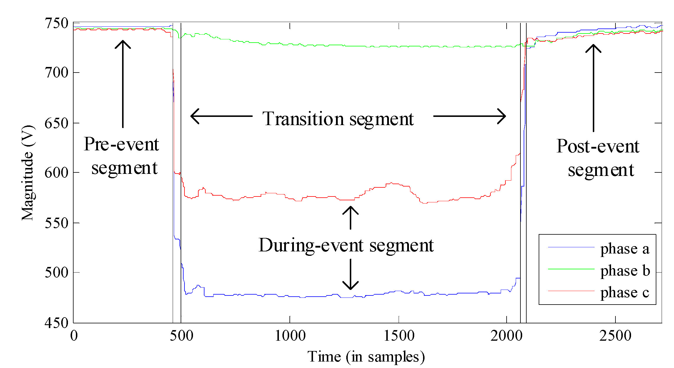
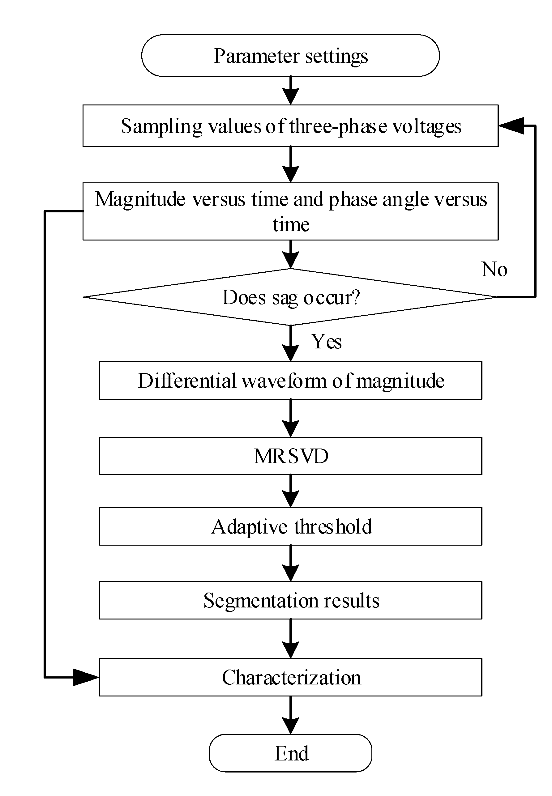
2. Application of the Segmentation Method to a Voltage Sag Waveform Analysis
3. Transition Segment Detection Based on the Multi-Resolution Singular Value Decomposition Method
3.1. The Definition and Original Cause of Transition Segments
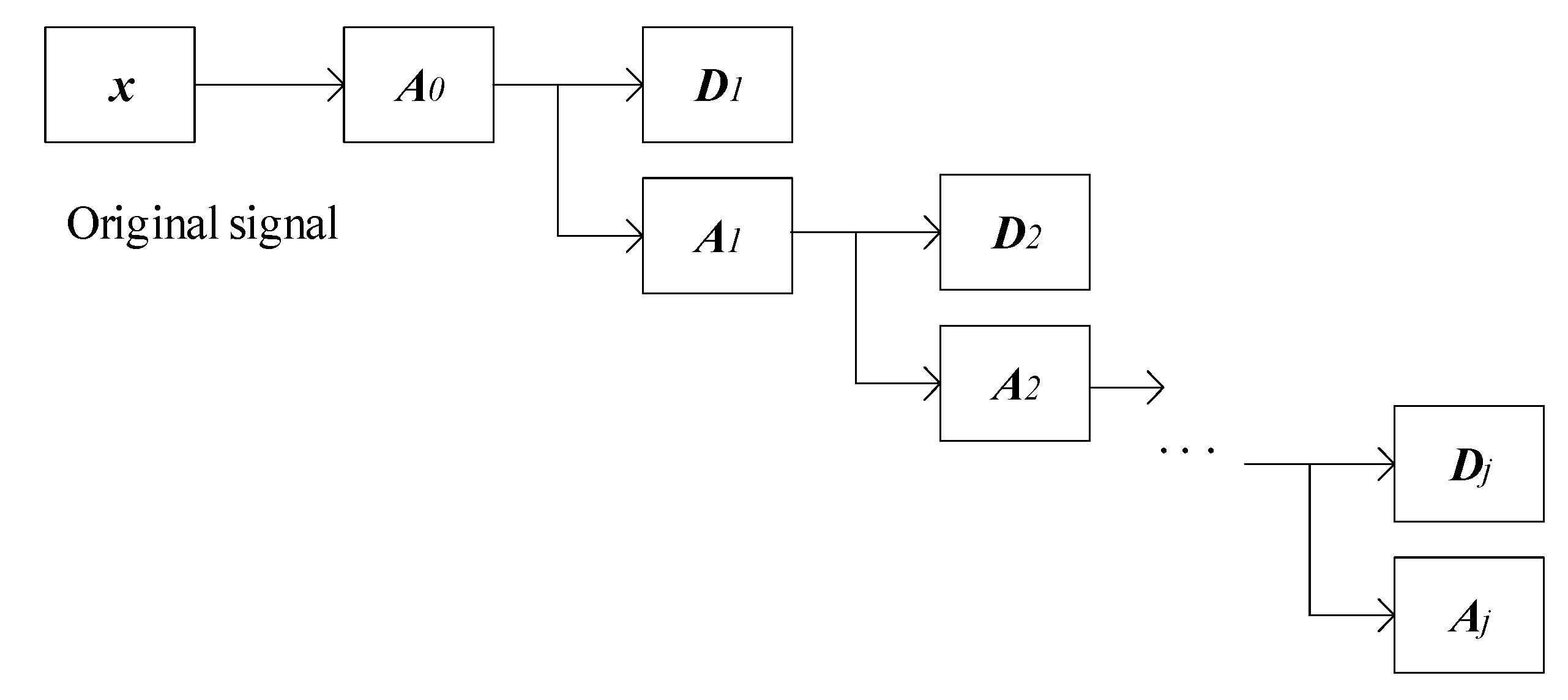
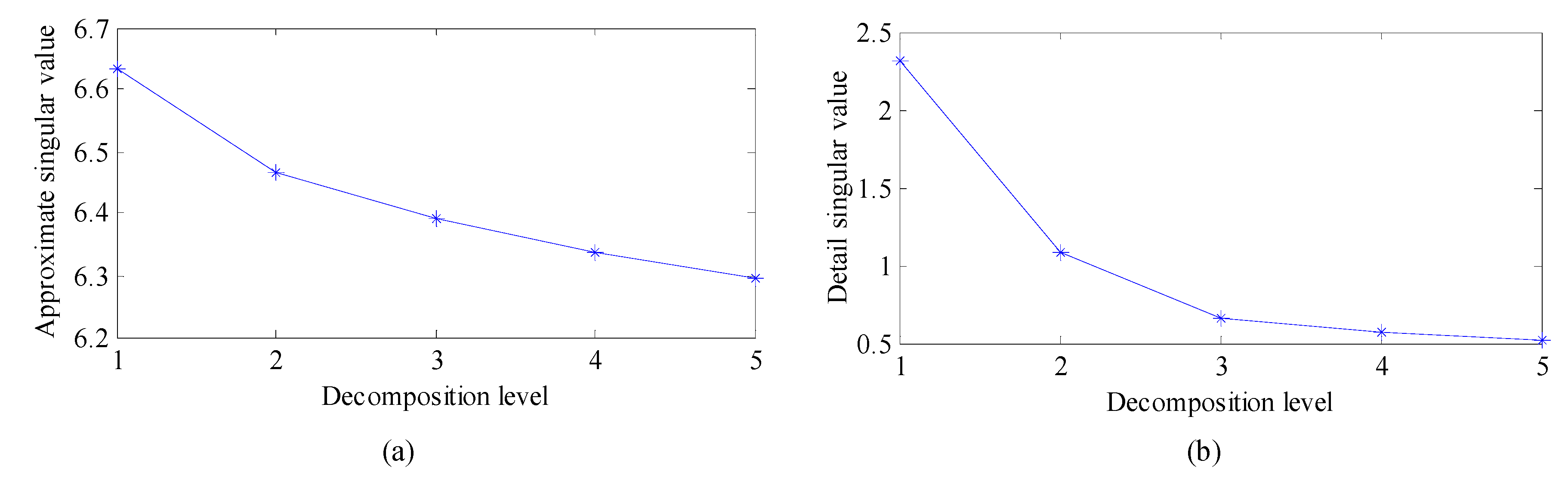
3.2. The Multi-Resolution Singular Value Decomposition Method
- (1)
- Construct a Hankel matrix A0 of an original signal x as:where is the input data sequence. After SVD, only two singular values are obtained, i.e., , and A0 is decomposed as:where
- (2)
- Construct the approximation component A1 and detail component D1 as:where La1 and La2 can be constructed from Equations (12) and (13), respectively. Similarly, Ld1 and Ld2 are constructed from Equations (14) and (15).
- (3)
- Repeating step (2) can obtain a series of detail components at each level, so multi-resolution decomposition is achieved. Finally, A0 in Equation (4) is decomposed as
4. Automatic Segmentation with an Adaptive Threshold
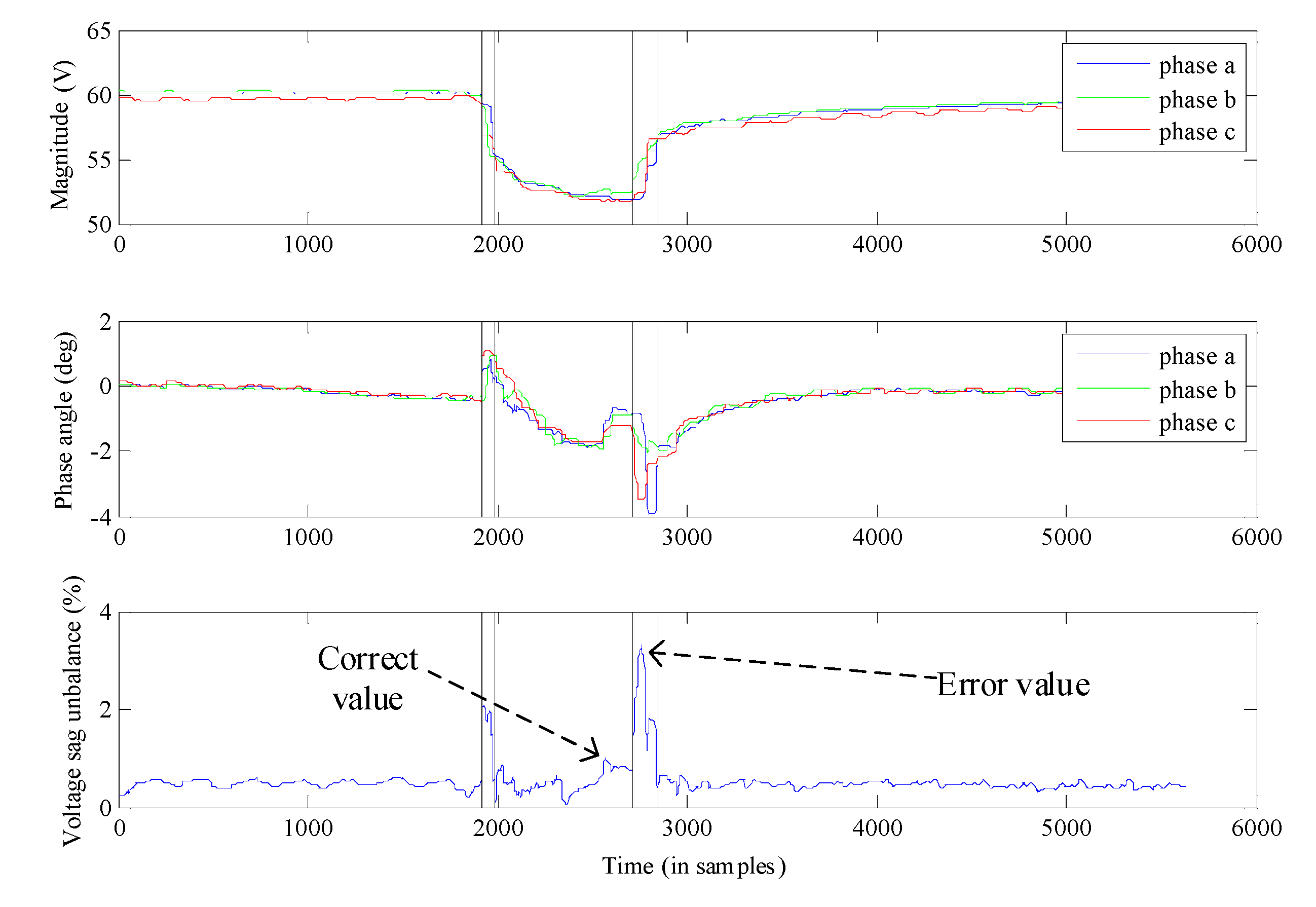
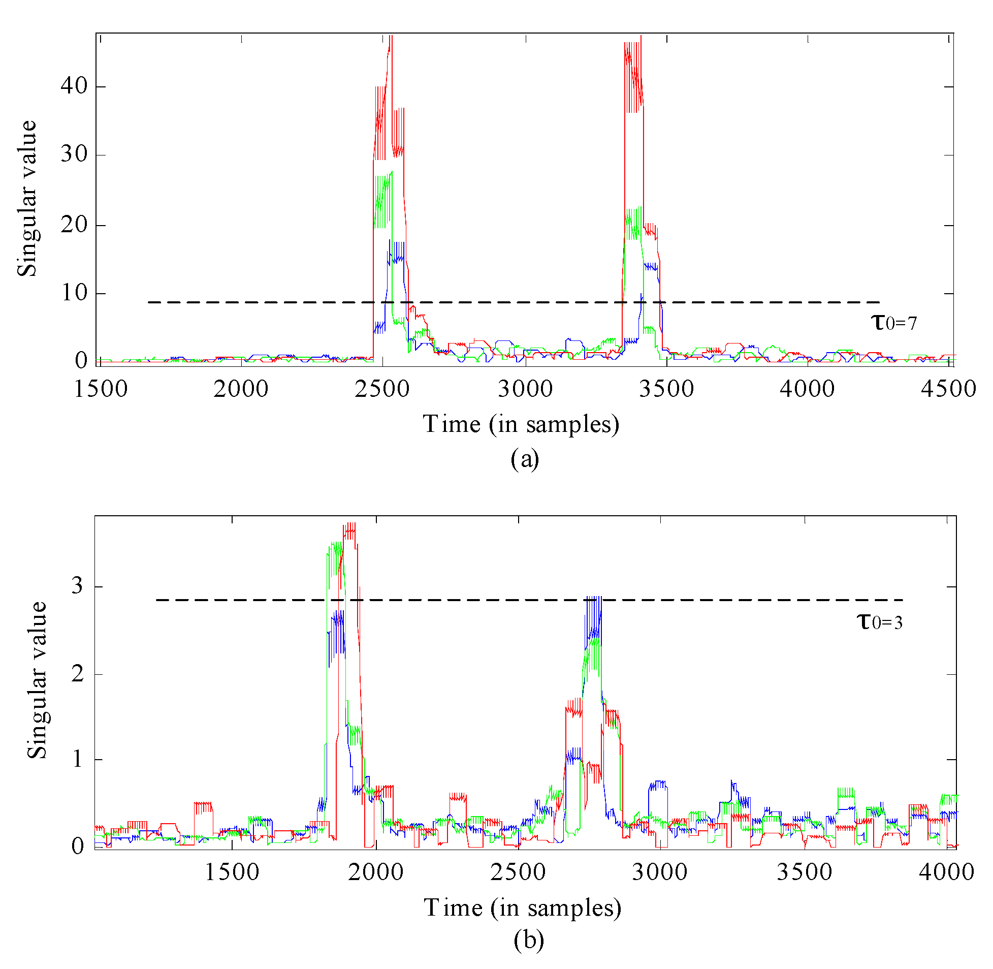
4.1. Impacts of a Constant Threshold Value on Segmentation
4.2. Construction Process of an Adaptive Threshold
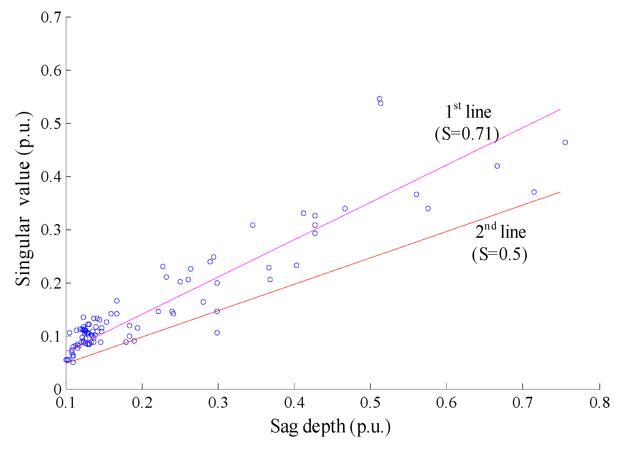
4.2.1. Sag Depth
4.2.2. Mean Square Error
4.2.3. Entropy
5. Results and Discussion
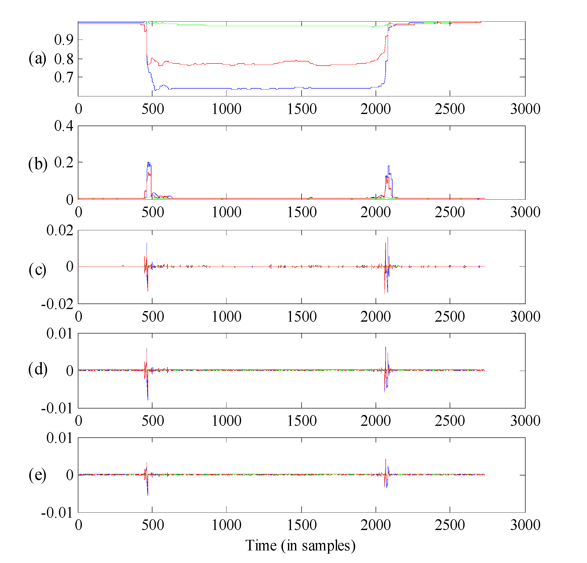
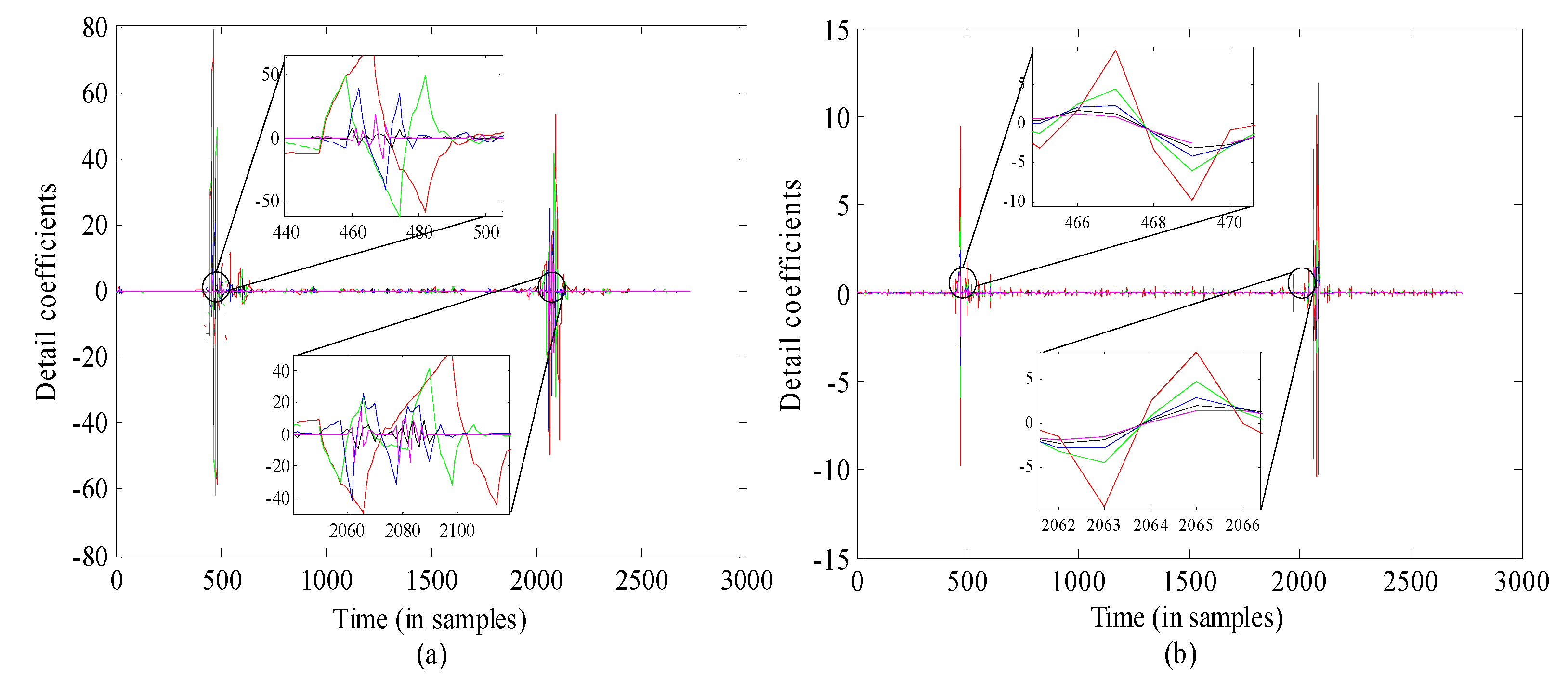
5.1. Performance of MRSVD in Transition Segments Detection
5.1.1. Transition Segment Detection
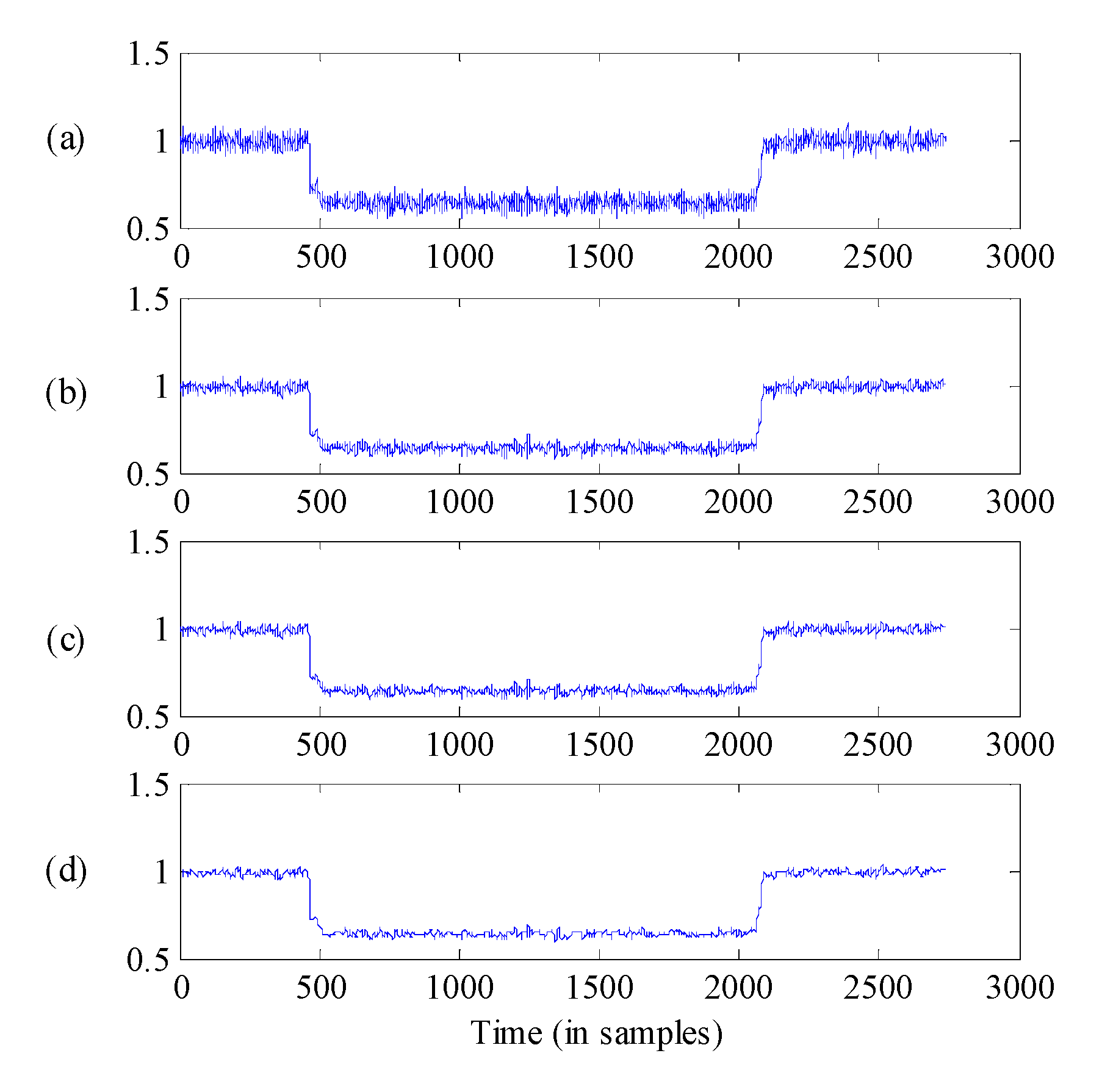
5.1.2. Denoising Capability
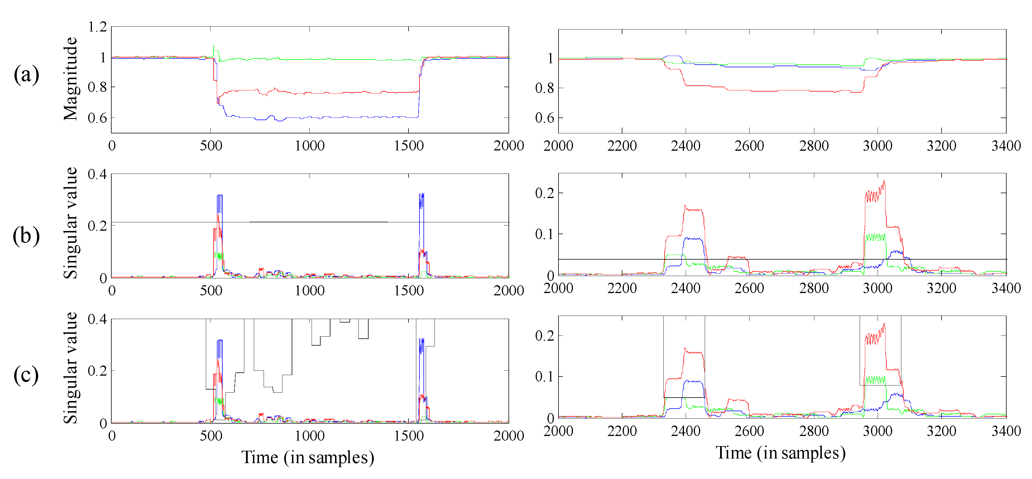
5.2. Performance of Segmentation with an Adaptive Threshold
5.2.1. Validation of the Adaptive Threshold
5.2.2. The Effectiveness of the Proposed Method Compared to an Existing Method
6. Conclusions
Author Contributions
Funding
Acknowledgments
Conflicts of Interest
Nomenclature
| A | Hankel matrix constructed by input signal. |
| U | Left singular vector in singular value decomposition |
| V | Right singular vector in singular value decomposition |
| S | Diagonal matrix of eigenvalues arranged in decreasing order |
| x | Input signal |
| λ | Singular value |
| j | Decomposition level |
| dj | Detail coefficient at each decomposition level |
| σ | Singular value |
| σa | Approximation singular value |
| σd | Detail singular value |
| Aj | Approximation component |
| Dj | Detail component |
| La | Subvector of approximation component |
| Ld | Subvector of detail component |
| τ0 | Constant threshold value |
| τ | Adaptive threshold value |
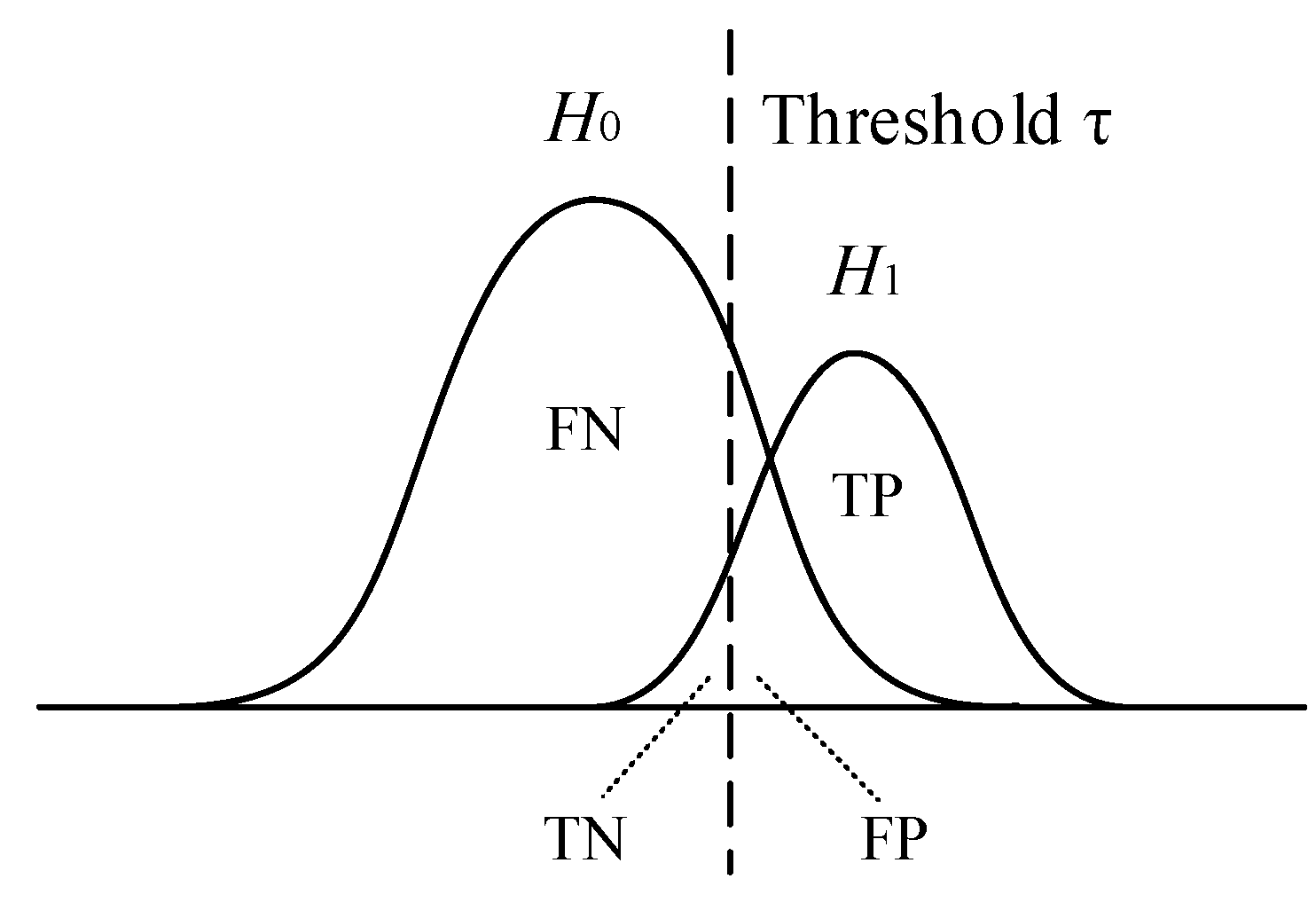
| TP | Number of correctly detected cases |
| TN | Number of miss alarm cases |
| FP | Number of false alarm cases |
| FN | Number of correctly undetected cases |
| Vdepth | Sag depth |
| VN | Nominal voltage |
| Vmin | Minimum voltage during sag event |
| MSE | Mean square error |
| vi | Fundamental voltage sequence |
| Mean value of all voltage values in a calculation window | |
| k | Calculation window size for MSE and entropy |
| ES | Entropy of singular values |
| Smax | maximum of nominal entropy value |
| Pj | Energy ratio at each decomposition level |
| ET | Total energy of signal |
| Ej | Sum of energy at each decomposition level |
| Sensitivity(S1) | Proportion of correctly detected cases among all of true cases |
| Specificity(S2) | Proportion of correctly undetected cases among all of false cases |
References
- IEC. Electromagnetic Compatibility (EMC): Part 4-30: Testing and Measurement Techniques—Power Quality Measurement Methods; IEC 61000-4-30 Ed 3.0; International Electrotechnical Commission: Geneva, Switzerland, 2015. [Google Scholar]
- IEEE. IEEE Recommended Practice for Monitoring Electric Power Quality; IEEE 1159 Ed 2.0; Institute of Electrical and Electronics Engineers: New York, NY, USA, 2009. [Google Scholar]
- IEC. Electromagnetic Compatibility (EMC): Part 2: Environment-Voltage Dips and Short Interruptions on Public Electric Power Supply Systems with Statistical Measurement Results; IEC 61000-2-8 Ed 2.0; International Electrotechnical Commission: Geneva, Switzerland, 2014. [Google Scholar]
- IEEE. IEEE Guide for Voltage Sag Indices; IEEE 1564-2014; Institute of Electrical and Electronics Engineers: New York, NY, USA, 2014. [Google Scholar]
- Mahela, O.P.; Shaik, A.G.; Gupta, N. A critical review of detection and classification of power quality events. Renew. Sustain. Energy Rev. 2015, 41, 495–505. [Google Scholar] [CrossRef]
- Bollen, M.H.J.; Gu, I.Y.H. Signal Processing of Power Quality Disturbances; John Wiley & Sons: Hoboken, NJ, USA, 2006. [Google Scholar]
- CIGRE/CIRED/UIE JWG C4.110. Voltage Dip Immunity of Equipment and Installations. CIGRE Technical Brochure TB 412. 2010. Available online: http://www.uie.org/sites/default/files/CIGRE%20TB412%20voltage%20dip%20immunity%20of%20equipment%20and%20installations.pdf (accessed on 17 December 2018).
- Begheri, A.; Bollen, M.H.J.; Gu, I.Y.H. Improved characterization of Multi-Stage Voltage Dips based on the Space Phasor Model. Electr. Power Syst. Res. 2018, 154, 319–328. [Google Scholar] [CrossRef]
- Wang, Y.; Bagheri, A.; Bollen, M.H.; Xiao, X.Y. Single-Event Characteristics for Voltage Dips in Three-Phase Systems. IEEE Trans. Power Deliv. 2017, 32, 832–840. [Google Scholar] [CrossRef]
- Wang, Y.; Bollen, M.H.J.; Xiao, X.Y. Calculation of the Phase-Angle-Jump for Voltage Dips in Three-Phase Systems. IEEE Trans. Power Deliv. 2015, 30, 480–487. [Google Scholar] [CrossRef]
- Ignatova, V.; Granjon, P.; Bacha, S. Space vector method for voltage dips and swells analysis. IEEE Trans. Power Deliv. 2009, 24, 2054–2061. [Google Scholar] [CrossRef]
- Lazaro, E.G.; Fuentes, J.A.; Garcia, A.M.; Carreton, M.C. Characterization and visualization of voltage dips in wind power installations. IEEE Trans. Power Deliv. 2009, 24, 2071–2078. [Google Scholar] [CrossRef]
- Styvaktakis, E.; Bollen, M.H.J.; Gu, I.Y.H. Expert System for Classification and Analysis of Power System Events. IEEE Trans. Power Deliv. 2002, 17, 423–428. [Google Scholar] [CrossRef]
- Garcia, I.M.M.; Munoz, A.M.; Castro, A.G.; Bollen, M.; Gu, I.Y.H. Novel Segmentation Technique for Measured Three-Phase Voltage Dips. Energies 2015, 8, 8319–8338. [Google Scholar] [CrossRef] [Green Version]
- Djokic, S.Z.; Milanovic, J.V.; Rowland, S.M. Advanced voltage sag characterisation II: Point on wave. IET Gener. Transm. Dis. 2007, 1, 146–154. [Google Scholar] [CrossRef]
- Pedra, J.; Sainz, L.; Córcoles, F.; Bergas, J.; Blas, A.D. Effects of balanced and unbalanced voltage sags on DC adjustable-speed drives. Electr. Power Syst. Res. 2008, 78, 957–966. [Google Scholar] [CrossRef]
- Nagata, E.A.; Ferreira, D.D.; Duque, C.A.; Cequeira, A.S. Voltage sag and swell detection and segmentation based on Independent Component Analysis. Electr. Power Syst. Res. 2018, 155, 274–280. [Google Scholar] [CrossRef]
- Rabiner, L.R.; Schafer, R.W. Digital Processing of Speech Signals; Prentice-Hall: Englewood Cliffs, NJ, USA, 1978. [Google Scholar]
- Hsin, L.T.; Gibson, J.D. Speech analysis and segmentation by parametric filtering. IEEE Trans. Speech Audio Process. 1996, 4, 203–213. [Google Scholar]
- Kakarala, R.; Ogunbona, P.O. Signal analysis using a multiresolution form of the singular value decomposition. IEEE Trans. Image Process. 2001, 10, 724–735. [Google Scholar] [CrossRef] [PubMed]
- Bhatnagar, G.; Saha, A.; Wu, Q.M.J.; Atrey, P.K. Analysis and extension of multiresolution singular value decomposition. Inf. Sci. 2014, 277, 247–262. [Google Scholar] [CrossRef]
- Malini, S.; Moni, R.S. Image denoising using multiresolution singular value decomposition transform. Procedia Comput. Sci. 2015, 46, 1708–1715. [Google Scholar] [CrossRef]
- Akobeng, A.K. Understanding diagnostic tests 3: Receiver operating characteristic curves. Acta Paediatr. 2007, 96, 644–647. [Google Scholar] [CrossRef]
- Chang, S.G.; Yu, B.; Vetterli, M. Adaptive wavelet thresholding for image denoising and compression. IEEE Trans. Image Process. 2000, 9, 1532–1546. [Google Scholar] [CrossRef] [PubMed] [Green Version]
- Ren, W.X.; Sun, Z.S. Structural damage identification by using wavelet entropy. Eng. Struc. 2008, 30, 2840–2849. [Google Scholar] [CrossRef]
- Rosso, O.A.; Blanco, S.; Yordanova, J.; Kolev, V.; Figliola, A.; Schürmann, M.; Basar, E. Wavelet entropy: A new tool for analysis of short duration brain electrical signals. J. Neurosci. Methods 2001, 105, 65–75. [Google Scholar] [CrossRef]


| Physical Truth | Positive (Transition Segment) | Negative (Steady Segment) |
|---|---|---|
| True (Transition segment) | TP | TN |
| False (Steady segment) | FP | FN |
| τ (10−4) | Constant Threshold | Adaptive Threshold | ||
|---|---|---|---|---|
| S1 | S2 | S1 | S2 | |
| 1.0 | 87.78 | 72.22 | 92.22 | 85.56 |
| 1.5 | 85.56 | 76.67 | ||
| 2.0 | 82.22 | 81.11 | ||
| 2.5 | 78.89 | 83.33 | ||
| 3.0 | 75.56 | 84.44 | ||
© 2018 by the authors. Licensee MDPI, Basel, Switzerland. This article is an open access article distributed under the terms and conditions of the Creative Commons Attribution (CC BY) license (http://creativecommons.org/licenses/by/4.0/).
Share and Cite
Xiao, X.; Hu, W.; Zhang, H.; Ai, J.; Zheng, Z. An Adaptive Approach for Voltage Sag Automatic Segmentation. Energies 2018, 11, 3519. https://doi.org/10.3390/en11123519
Xiao X, Hu W, Zhang H, Ai J, Zheng Z. An Adaptive Approach for Voltage Sag Automatic Segmentation. Energies. 2018; 11(12):3519. https://doi.org/10.3390/en11123519
Chicago/Turabian StyleXiao, Xianyong, Wenxi Hu, Huaying Zhang, Jingwen Ai, and Zixuan Zheng. 2018. "An Adaptive Approach for Voltage Sag Automatic Segmentation" Energies 11, no. 12: 3519. https://doi.org/10.3390/en11123519