Moving Average Market Timing in European Energy Markets: Production Versus Emissions

Abstract

This paper searches for stochastic trends and returns predictability in key energy asset markets in Europe over the last decade. The financial assets include Intercontinental Exchange Futures Europe (ICE-ECX) carbon emission allowances (the main driver of interest), European Energy Exchange (EEX) Coal ARA futures and ICE Brent oil futures (reflecting the two largest energy sources in Europe), Stoxx600 Europe Oil and Gas Index (the main energy stock index in Europe), EEX Power Futures (representing electricity), and Stoxx600 Europe Renewable Energy index (representing the sunrise energy industry). This paper finds that the Moving Average (MA) technique beats random timing for carbon emission allowances, coal, and renewable energy. In these asset markets, there seems to be significant returns predictability of stochastic trends in prices. The results are mixed for Brent oil, and there are no predictable trends for the Oil and Gas index. Stochastic trends are also missing in the electricity market as there is an ARFIMA-FIGARCH process in the day-ahead power prices. The empirical results are interesting for several reasons. We identified the data generating process in EU electricity prices as fractionally integrated (0.5), with a fractionally integrated Generalized AutoRegressive Conditional Heteroscedasticity (GARCH) process in the residual. This is a novel finding. The order of integration of order 0.5 implies that the process is not stationary but less non-stationary than the non-stationary I(1) process, and that the process has long memory. This is probably because electricity cannot be stored. Returns predictability with MA rules requires stochastic trends in price series, indicating that the asset prices should obey the I(1) process, that is, to facilitate long run returns predictability. However, all the other price series tested in the paper are I(1)-processes, so that their returns series are stationary. The empirical results are important because they give a simple answer to the following question: When are MA rules useful? The answer is that, if significant stochastic trends develop in prices, long run returns are predictable, and market timing performs better than does random timing.

1. Introduction

Climate change is possibly the most severe threat for human civilization, and greenhouse gas (GHG) emissions are considered to be a major market failure. Therefore, it is important to know how the price mechanism in financial markets accommodates the issue. This paper tackles the question by investigating whether there are differences in asset price predictability (and hence market efficiency) between different modes of energy sources. The energy sector is the main producer of GHG emissions (at 57% in 2016) in Europe [1]. The aim of the paper is to investigate price predictability of a main policy instrument, namely tradable emission allowances.

Europe created the world’s first carbon emission allowances trading system in 2005 [2]. The basic idea is simple, namely companies that produce carbon dioxide (CO₂) emissions must buy and show emission allowances enough to cover their yearly emissions, or heavy fines are sentenced. Holding one emissions allowance gives a permit to produce one ton of CO₂ emissions. The allowances are tradable, and market pricing of the emissions is supposed to guide companies to reduce their emissions efficiently [3]. Therefore, carbon emission allowances are inherently financial assets.

The EU Emissions Trading System (EU ETS) currently covers about 45% of all GHG emissions in the EU. The system operates in all EU countries, together with Norway, Iceland, and Liechtenstein, and has a co-operation agreement with the ETS of Switzerland [3]. In the system, a price cap is set by estimating total greenhouse gases produced by European companies during a multi-year phase, and is gradually diminished to reduce total emissions over time.

To date, the Commission has executed two emission allowance phases, namely phase 1 in 2005–2007, and phase 2 in 2008–2013. The ongoing phase 3 commenced in 2014, and is due to end in 2020, after which phase 4 will start. In phase 1, the firms received their allowance allocations for free, and the fine was 40 € per ton of CO₂ emissions. In phases 2 and 3, the fine was lifted to 100 € per ton. In phase 3, auctioning became the practice of allocating new allowances, and about 40% of new allowances were auctioned in 2017. The main auctions are held at the European Energy Exchange (EEX) in Germany, and Intercontinental Exchange Futures Europe (ICE-ECX). The latter emerged when the American ICE bought the European ECX in 2010. EEX also serves as the main trading place for coal, natural gas, and electricity in Continental Europe.

The paper is inspired by Ilomäki et al. [4], which uses DJIA stocks data from 1988 to 2017. The paper finds that market timing with MA rules outperforms buy and hold, when the frequency of used observations is reduced, and the whole rolling window size of 200 trading days is used. This paper investigates returns predictability with more specific financial assets. The aim is to examine whether market timing with moving averages (MA) [5] has been successful for the EU CO₂ emission allowances, EU coal future prices, Brent oil futures, Dow Jones Stoxx 600 Europe renewable energy index, Dow Jones Stoxx 600 Europe oil and gas index, and European power prices (the data are from Thomson Reuters Datastream).

The two European stock indices are distinctive to heavy and low GHG producers in the energy sector. The EU coal future prices are relevant as coal is the primary energy source, particularly in Germany. Currently, coal is ranked second after oil as an energy source in the world [6]. The trading in future contracts started on 26 February 2008 for phase 2. Following the literature, our data starts from that date, and ends on 28 September 2018.

The paper proceeds as follows. Section 2 provides a literature review, and Section 3 presents the model specifications. Section 4 reports the empirical analysis, and Section 5 provides some concluding remarks

2. Literature Review

The economics literature on GHG emissions has grown rapidly after the launch of EU ETS in 2005. Seifert et al. [7] argue that emission allowance prices should follow a martingale process with conditional heteroskedasticity. Yet, using daily trading data over the first two years, Paolella and Taschini [8] report that CO₂ emission allowance returns follow a first order autoregressive model with Generalized Autoregressive Conditional Heteroscedasticity (GARCH) disturbances [9,10], indicating an AR(1)-GARCH(1,1) process for log returns (for details on ARMA-GARCH modelling, see Reference [11]. This suggests short-term returns predictability, which violates the martingale hypothesis.

Moreover, Benz and Truck [12] found that the Markov switching model [13] of returns fits the EU CO₂ data, such that there is a stationary non-linear process in returns. Montagnoli and de Vries [14] note that there is significant returns predictability in phase 1, but a martingale process in phase 2. Their data on phase 2 covers the period 26 February 2008 to 4 April 2009, which is sourced from BlueNext trading scene (which was closed in 2012). Arouri et al. [15] argue that CO₂ spot and future prices have a non-linear relationship as there are asymmetric and non-linear relations between spot and future returns.

Daskalakis and Markellos [16] note that there is a carbon component in the market price of European electricity as there is a CO₂ emission allowance risk premium added to the price of electric power. Bublitz et al. [17] argue that the decline in carbon and coal prices has been the main driver of the fall in electricity prices in Germany and Continental Europe from 2011 to 2015. Veith et al. [18] report a positive correlation between CO₂ emission allowance returns and European energy sector returns.

Oestreich and Tsiakas [19] find that, in German stock markets, the free allocation of emission allowances created a carbon premium for those high carbon producers that produced significant amounts of GHG, but that the effect disappeared in 2009. Bushnell et al. [20] examined how the effect of the sharp decline in EU CO₂ emissions allowance prices in 2006 affected market valuations in the energy sector, and found that low carbon producers had suffered more than high carbon producers. Brouwers et al. [21] investigated the impacts of CO₂ emissions verification events on the stock returns of European companies, and note that the events have had a significant impact only on carbon-intensive companies.

Creti et al. [22] find that, in the early years of phase 2, CO₂ emissions allowance prices have been cointegrated [23] with basic fundamentals, namely with Brent oil, EuroStoxx 50 index, and with a switching price between coal and gas. However, Koch et al. [24] report that cointegration does not exist when data over the whole phase 2 are examined. Tian et al. [25] note that EU CO₂ returns correlate positively with European energy stocks returns, but negatively with carbon-intensive stocks returns. In addition, Charles et al. [26] find cointegration between EU CO₂ emissions spot and future prices, and interest rates, during phase 2.

More importantly, Daskalakis and Markellos [27] test market efficiency in EU CO₂ pricing with MA rules, namely with daily observations, MA50, MA30 and MA15. The conclusion is that returns were predictable in phase 1, possibly because of the lack of maturity of the market (At the end of phase 1, the market was in flux. According to the EU ETS, the financial crisis of 2007 created a major surplus of CO2 emissions allowances. At the beginning of December 2007, the equilibrium price in the secondary market plummeted to an all-time low of 0.01 to 0.03 € per CO2 ton, both in the EEX and ECX. The surplus led to an acute rise in imports of international emissions allowance credits that are also tradable in the EEX and ECX.). Daskalakis [28] re-tested market efficiency in emission (futures) prices in phase 2 with daily observations, using the MA15 rule. The finding is that the MA rule beats the buy and hold strategy in terms of the Sharpe ratio in 2008 and 2009, but not in 2010. This suggests a gradually improving market efficiency. However, Medina et al. [29] argue that improvement in efficiency (from phase 1 to phase 2) cannot be observed from intra-day data. Ibikunle et al. [30] used intra-day data for 2008–2011, and tested the correlation of liquidity and market efficiency in EU carbon emissions returns. The conclusion is that increasing liquidity has improved pricing efficiency, and that random walk pricing behaviour has emerged in 2010–2011.

Crossland et al. [31] find significant time series momentum up to 12 months with EU ETS returns between early 2008 and mid-2011. Moskowitz et al. [32] find significant time series momentum with crude oil future prices in monthly data from January 1985 to December 2009. Yin and Yang [33] used monthly data on crude oil future prices from 1984 to 2013, and found that MA rules and time series momentum rules outperform predictions based on macroeconomic variables. Liu et al. [34] drew the same conclusion using 10 MA rules with monthly data for 1986–2015.

Starting from Markowitz [35], rational investors are assumed to be risk averse, indicating that they monitor both returns and its variability. Sharpe [36] and Lintner [37] state that returns over riskless returns depend linearly and positively on market risk adjusted returns. However, LeRoy [38] and Merton [39] show that, if investors are risk averse, time-varying risk adjusted returns exist, and can be partly predictable because of the non-linear relationship between returns and variability.

Bearing this in mind, Malkiel [40] argues that efficient markets do not allow investors to gain above average returns without accepting above average variability in returns. Merton [41] argues that the decision when to buy stocks and when to sell them is insignificant in the long run, and random decisions cannot be beaten when markets are efficient. This is based on the idea that future information shocks are unpredictable, and non-stationarity of competitive prices tends to develop stochastic trends that could change unexpectedly due to new information.

Zhu and Zhou [42] showed analytically that MA rules add value for a risk averse investor if returns are predictable. The empirical literature on predictability with MA rules is extensive. For example, Neely et al. [43], Ni et al. [44], and Marshall et al. [45] found that investors benefit from the use of MA rules, whereas Hudson et al. [46] claim that MA rules are useless in intra-day trading. The main inspiration for this paper comes from the findings in Chang et al. [47] that the DJIA index returns are predictable in the long run according to MA rules, which provides empirical support for the analytical result in Reference [42].

Neto et al. [48] propose a methodology for risk analysis and portfolio optimization of power generation assets in Brazil with hydro, wind, and solar power. Innovative stochastic models are used to generate synthetic time series for water inflow, wind speed, solar irradiance, temperature of the photovoltaic panel, and average generation capacity of energy. The simulation is implemented using Monte simulations with a Cholesky decomposition. An economic approach is presented, taking into account taxation and financing, as well as Markowitz portfolio theory. The results show that the correlation between energy resources is altered by cash flows and debt. In the diversification process, the complementarity between sources reduces economic risk. The increase in debt increases the correlation, decreases return and risk, and affects the diversification results. This significantly reduces the hydroelectric economic risk and increase the financial return, which directly benefits the formation of portfolios.

Rezec and Scholtens [49] note that the support of financial markets for the transformation of the energy system to a low carbon society seems critical for its success, and may depend on market incentives. The authors analyze how equity indices that capture renewable energy investments perform compared to conventional benchmark indices, especially financial market investors, such as pension funds, insurance companies, and mutual funds that use these to assess and guide their renewable energy investments. The authors consider financial market participants that invest indirectly in renewable energy as an example of market environmentalism with respect to commodification and frame-shifting. It is found that that the renewable energy indices’ risk-adjusted return is poor, so that renewable energy does not seem to be a financially attractive portfolio investment.

Ferreira et al. [50] consider an investment whereby agents are interested in obtaining returns but prefer less risky assets. There are other that might influence this selection. Retrieving information for 26 shares of firms that produce renewable energy, the authors use the DCCA correlation coefficient to see how those shares behave with the main indices. If shares and indices are not correlated, different factors could be seen as risk diversification. The results show that in the short run correlation exists (in scales under 100 days), but in the long run most shares are uncorrelated with the indices of their countries (in scales greater than 200). This means that shares associated with more sustainable principles could be used to manage portfolio risks.

3. Model Specification

The theoretical model closely follows Ilomäki et al. [4], and Chang et al. [47]. We consider all the energy stocks as financial assets, and assume risk averse investors live for two periods in an overlapping generations economy with a continuum of young and old investors $\left[0,1\right]$. An investor opens a position in period one, and closes the position in period two, when all wealth is consumed. A young investor j allocates initial wealth $w_t^j$ between infinitely-lived risky assets, $i=1,2,3,\dots I,$ and risk-free assets that produce the risk-free rate return, r^f. A risky asset $i$ may pay dividend $D_t^i$, and has $x_i^s$ outstanding. A young investor $j$ maximizes utility from old age consumption through optimal allocation of initial resources, $w_t^j$, between risky and risk-free assets.

Ignoring the correlation between risky assets, and concentrating on each risky asset separately, a young investor j maximizes utility with respect to each risky asset i:

$$\begin{array}{l}\max x_t^{ij}\left(\frac{E_t(P_{t+1}^i+D_{t+1}^i)}{P_t^i}-(1+r^f)\right)-\frac{{\nu }^j}{2}{x}^{i{j}^2}{\sigma }_i^2\\ s.t.\\ x_t^{ij}{P}_t^i\le w_t^j\end{array}$$

where $E_t$ is the expectations operator, $P_t^i$ is the price of one share of asset $i$, ${\nu }^j$ > 0 is a constant risk-aversion parameter for investor $j$, ${\sigma }_i^2$> 0 is the variance of returns for the risky asset $i$, and $x_t^{ij}$ is the investor’s demand for risky asset $i$. The first-order condition yields:

$$x_t^{ij}=\frac{E_t\left((P_{t+1}^i+D_{t+1}^i)/P_t^i\right)-(1+r^f)}{{\nu }^j{\sigma }_i^2}$$

(1)

for investor j’s optimal demand for the risky asset i. Suppose that the investor uses MA rules for market timing, and allocates initial wealth, $w_t^j$, between each risky asset and the risk-free asset according to the MA rule forecast about the return of the asset. The investor invests in the risky asset $i$ only if the numerator on the right-hand side of Equation (1) is positive, that is, if $E_t\left((P_{t+1}^i+D_{t+1}^i)/P_t^i\right)>(1+r^f)$ holds.

4. Empirical Analysis

The sample data consists of daily prices from 26 February 2008 to 28 September 2018. In choosing the data period, we followed the common practice in the energy economics literature [14,27], and excluded phase 1 because of evident issues during that period. This reduces the chances of structural change during the sample period. Trading with EU CO₂ emissions allowances in ICE-ECX started at the beginning of phase 2, that is, on 26 February 2008. The basic rolling window is the first 200 trading days, which means that the data analysis starts from 2 December 2008 and ends on 28 September 2018, yielding 2564 daily observations. We report the variables in Euros, except for Coal ARA and Brent Crude Oil futures, which are reported in USD.

The Augmented Dickey–Fuller (ADF) test shows that CO₂ emissions futures, Coal futures, Brent Oil futures, Stoxx 600 Europe Renewable Energy Index, and Stoxx 600 Europe Oil and Gas Index are integrated of order one, I(1). This indicates that the natural logarithm returns of these series are stationary. The EEX Power Futures is the electricity market place for Germany, Austria, France, Italy, Spain, Holland, Czech Republic, Belgium, Switzerland, Poland, Nordic countries, Hungary, Romania, Slovak Republic, and the UK.

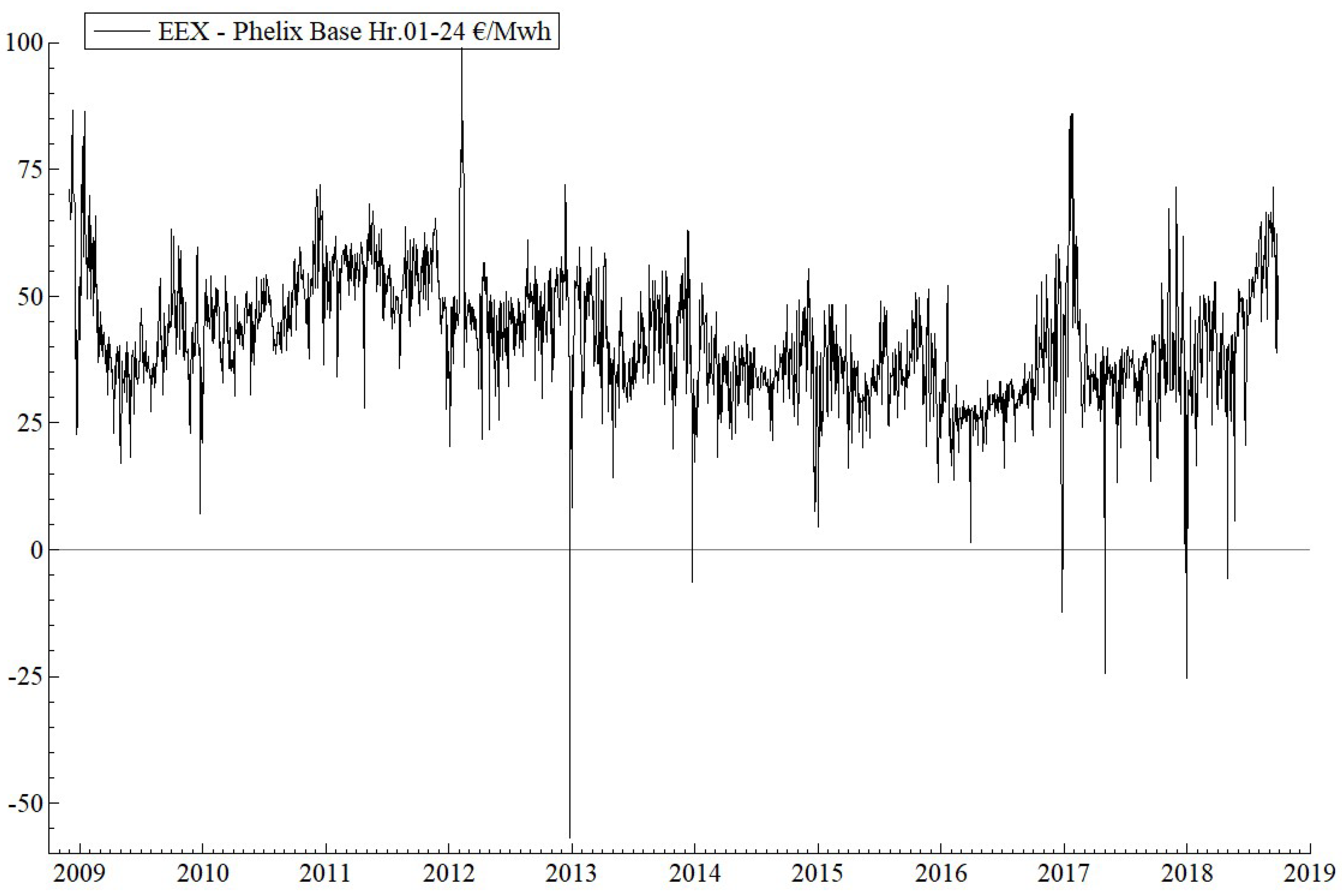
Figure 1 shows that the Phelix-DE Power future prices (base 1–24 h) are stationary, that is, I(0), with an ADF test value of −12.79. The eight negative Phelix prices are concentrated during the holiday seasons, namely 12/25/2012, 12/26/2012, 12/24/2013, 12/26/2016, 5/1/2017, 12/26/2017, 1/1/2018 and 5/1/2018. According to the European Energy Exchange, negative power prices occur when a high and inflexible (nuclear/lignite) power generation appears simultaneously with low electricity demand. This is often the case on public holidays such as Christmas. In hours of renewable power supply (wind and sun), power producers offer their electricity for negative prices on the exchange. This is often done by marketers of renewable power, but also by conventional power stations like nuclear and lignite plants. In this event, the market clearing price can be set below zero. In Germany, renewables have unlimited priority over fossil generation.

The equilibrium price of electrical power may produce stable equilibria as electricity cannot be stored. The average price is 41.55 € per Mwh, with standard deviation 11.88 €, and −56.87 € is the minimum and 98.98 € is the maximum price during the period. Note that there are some negative observations, usually during holiday seasons. This is simply because the generation of renewable energy exceeds demand in the grid, and the renewables have unlimited priority over fossil energy sources in Germany. The skewness of the stationary distribution is 0.270, and the kurtosis is 7.201. As electricity prices follow a stationary process, there cannot be any long-term stochastic trends. Therefore, random timing should be superior in the long run.

However, as reported in

Table 1. Electricity futures prices (Phelix-DE, base 1–24 h) estimated by Baillie-Bollerslev-Mikkelsen method [53], 2 December 2008 to 28 September 2018.

Parameters	Coefficient	Std.Error	t-value	t-prob
d ARFIMA	0.52	0.03	17	0.000
MA-1	0.08	0.04	2	0.021
Constant (Mean)	49.63	11.58	4	0.001
Constant (Var)	2.61	0.94	3	0.006
d-FIGARCH	0.58	0.11	5	0.000
phi	0.32	0.10	3	0.001
beta	0.59	0.10	6	0.000

below, the power price series is fractionally integrated. Thus, we can identify a fractionally integrated autoregressive moving average process, ARFIMA (for details of ARFIMA modelling, see Reference [51]). The empirical results indicate that the series has both long memory (that creates high correlation between events that are remote in time), and short memory (which lasts only one day, as a shock from the preceding day affects the present price). The ARFIMA (1,d,1) model can be specified as ${\left(1-L\right)}^d{z}_t={\beta }_1{\left(1-L\right)}^d{z}_{t-1}+{\epsilon }_t+{\beta }_2{\epsilon }_{t-1}$, where $L$ is the lag operator, indicating that ${\left(1-L\right)}^d={\mathsf{\Delta }}^d$, ${\epsilon }_t\sim NID(0,{\sigma }_{\epsilon }^2)$, $z_t=y_t-\mu$, that is, the mean $\mu$ is subtracted from the original series, $y_t$, ${\beta }_1$ and ${\beta }_2$ are the estimated parameters, and d is the order of fractional integration.

If $0<d<0.5$, the process is covariance stationary with long memory, assuming that the original ARMA process is covariance stationary [51,52] defines that, for $0.5\le d<1$ the series is not stationary, but less non-stationary than if d = 1. The variance also contains a fractionally integrated process, thereby suggesting an ARFIMA(0,d,1)-FIGARCH(1,d,1) model that yields non-autocorrelated and homoscedastic residuals. The FIGARCH process in the residual, ${\epsilon }_t$, is $h_t={\alpha }_0{(1-\beta (1))}^{-1}+\left[1-{(1-{\beta }_{1}L)}^{-1}(1-{\varphi }_{1}L){(1-L)}^d\right]{\epsilon }_t^2$, where $h_t$ is the conditional variance of ${\epsilon }_t$, and ${\alpha }_0,\varphi ,\beta$ are estimated parameters. The FIGARCH process implies that the influence of lagged squared residuals slows at a hyperbolic rate [53].

Table 1 shows that, if we take into account the long memory (at 0.5) and short memory parameters (at 0.1), the average power price has been 50 € per Mwh within the period.

Note that the MA of Gartley [5] is different from the MA process of Box and Jenkins [54] that is present in the ARFIMA estimation. The MA of Gartley detects stochastic trends in the non-stationary price series, thereby producing a non-stationary process, whereas the MA of Box and Jenkins is always a stationary process with short memory.

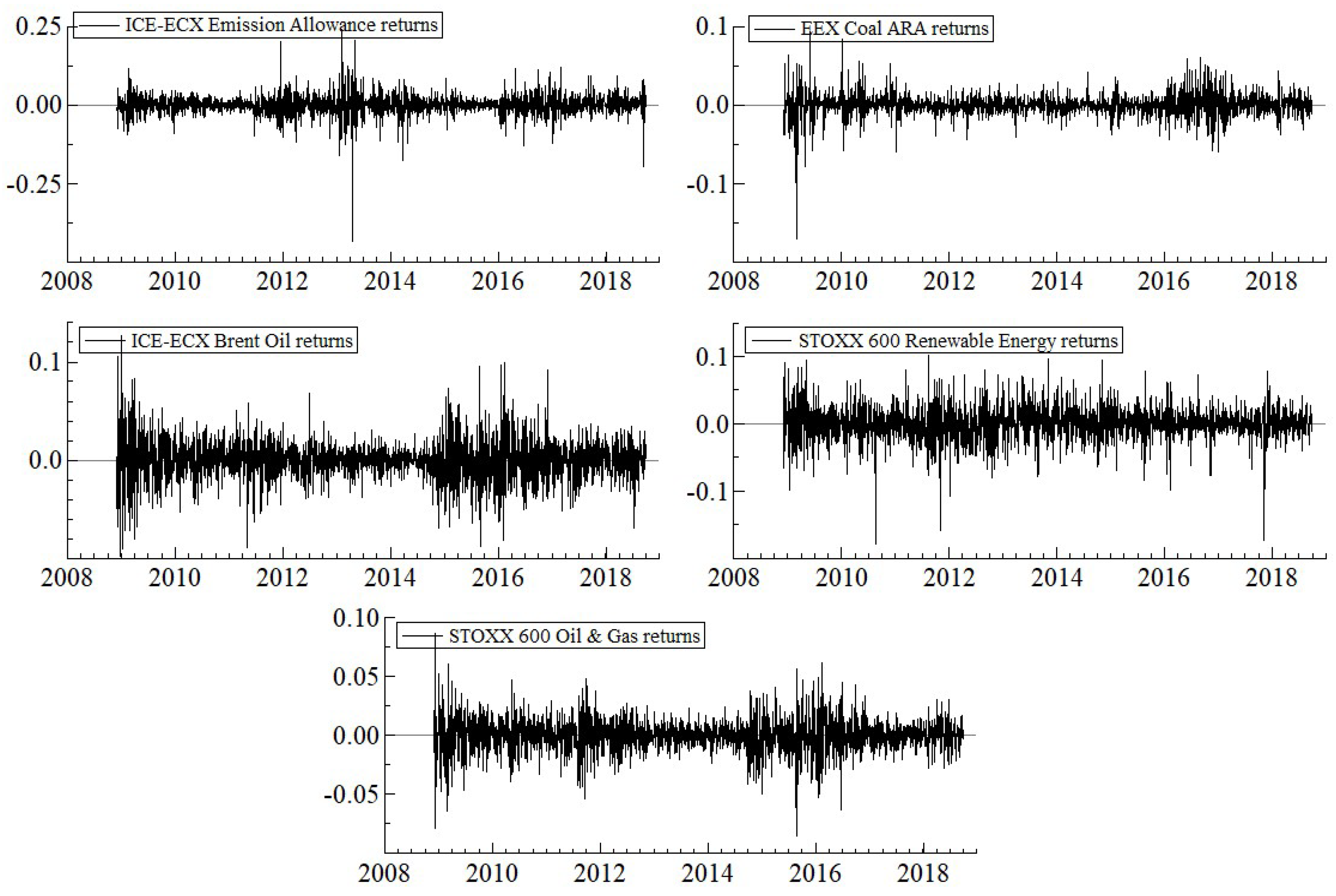
Figure 2 illustrates the log returns of ICE-ECX CO₂ EU emission allowances, EEX coal futures, ICE-ECX Brent oil futures, Dow Jones Stoxx 600 Europe Renewable Energy, and Oil and Gas Indices for ten years. The ADF tests reveal that all processes are stationary, that I, I(0).

Table 2. Descriptive statistics for log returns on carbon dioxide emission allowances, coal, Brent oil, Stoxx 600 Europe renewable energy index with dividends, Stoxx600 Europe Oil and Gas index with dividends, 2 December 2008 to 28 September 2018.

Variable	Mean	Standard Deviation	Skewness	Kurtosis	Obs.	Jarque-Bera	Sharpe Ratio
CO2 e. a.	0.031	0.514	−0.906	21.075	2564	35255	0.05
Coal	0.025	0.214	−0.607	18.459	2564	25690	0.10
Brent Oil	0.051	0.323	−0.154	6.538	2564	1347	0.15
Renew Energy Index	−0.025	0.386	−0.371	7.332	2564	2064	−0.08
Oil and Gas index	0.070	0.218	−0.166	6.431	2564	1269	0.30

provides descriptive statistics of the series in Figure 2. We used the three month Euribor (from Thomson Reuters Datastream) as the risk-free rate, yielding +0.004 for average annualized returns during the period. The Sharpe ratio is calculated as $[r_i-0.004]/{\sigma }^i=S{R}_i$, where $r_i$ is the average annualized returns with dividends, and ${\sigma }_i$ is the annualized daily volatility of returns for asset $i$.

Table 2 shows that the average annualized returns (with dividends) of the Oil and Gas stocks index is 0.070, with annualized volatility 0.218. It yields the best annualized Sharpe Ratio of 0.30 for the period. CO₂ emissions allowances yield a Sharpe ratio of 0.05, and coal 0.10, Brent oil 0.15, while that of the Renewable Energy Stock Index is −0.08. These outcomes show that renewable energy stocks have actually produced a negative return to risk value over the last decade in Europe, while fossil energy stocks have performed well.

Chang et al. [47] and Ilomäki et al. [51] find that market timing with MA rules adds value for a risk averse investor, as compared with random timing for Dow Jones Industrial Average stocks, and with the DJIA index itself. We followed the same procedure by choosing a 200 trading days rolling window so that the sample size of each asset sums to 2564 daily observations. We calculated the empirical results with seven frequencies for the MA rule. When the MA turns lower (higher) than the current daily closing price, we invest in the risky asset (three-month Euribor) at the closing price of the next trading day. Therefore, the market timing strategy is to invest all wealth, either in risky or risk-free assets, while the MA rule advises on the timing.

The first frequency rule is to calculate MA for every trading day; the second frequency rule takes into account every fifth trading day (proxy for weekly rule); the third frequency rule is for every 22nd trading day (proxy for monthly rule); the fourth frequency rule is for every 44th trading day (proxy for every second month); the fifth frequency rule is for every 66th trading day (proxy for every third month); the sixth frequency rule is for every 88th trading day (proxy for every fourth month); and the seventh frequency rule takes into account every 110th trading day (proxy for every fifth month).

For each asset, the MA rules produce 2564 × 9 = 23,076 daily returns for the first three frequencies, 2564 × 4 = 10,256 daily returns for the fourth rule, 2564 × 3 = 7692 daily returns for the fifth rule, 2564 × 2 = 5128 daily returns for the sixth rule, and 2564 daily returns for the seventh rule. At the first frequency (every trading day), we calculate daily returns for MA200, MA180, MA160, MA140, MA120, MA100, MA80, MA60, and MA40.

These are calculated as:

$$\left(\frac{P_{t-1}+P_{t-2}+\dots +P_{t-200}}{200}\right)=X_{t-1};$$

$$\left(\frac{P_{t-1}+P_{t-2}+\dots +P_{t-180}}{180}\right)=X_{t-1};$$

$$\left(\frac{P_{t-1}+P_{t-2}+\dots +P_{t-160}}{160}\right)=X_{t-1};$$

$$\left(\frac{P_{t-1}+P_{t-2}+\dots +P_{t-140}}{140}\right)=X_{t-1};$$

$$\left(\frac{P_{t-1}+P_{t-2}+\dots +P_{t-120}}{120}\right)=X_{t-1};$$

$$\left(\frac{P_{t-1}+P_{t-2}+\dots +P_{t-100}}{100}\right)=X_{t-1};$$

$$\left(\frac{P_{t-1}+P_{t-2}+\dots +P_{t-800}}{80}\right)=X_{t-1}$$

$$\left(\frac{P_{t-1}+P_{t-2}+\dots +P_{t-60}}{60}\right)=X_{t-1};$$

and

$$\left(\frac{P_{t-1}+P_{t-2}+\dots +P_{t-40}}{40}\right)=X_{t-1}$$

If $X_{t-1}<P_{t-1}$, we buy the stock at the closing price, $P_t$, giving $R_{t+1}=\ln \left(\frac{P_{t+1}}{P_t}\right)$ for daily returns. The transaction cost is 0.01% per transaction for all MA rule calculations.

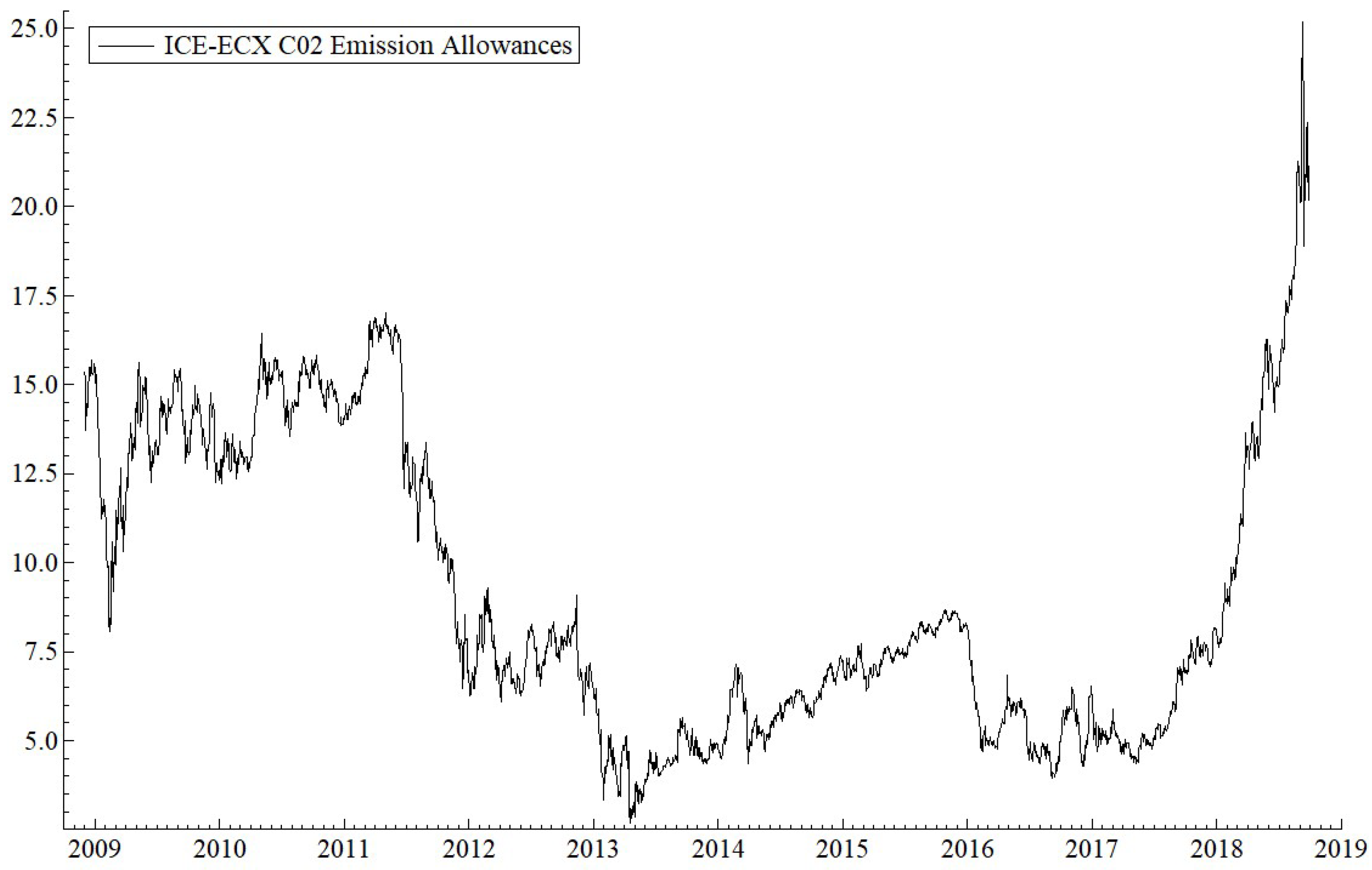
Figure 3 shows the European Carbon Emission Allowance prices, starting from 200 trading days after the beginning of phase 2, that is, from 2 December 2008.

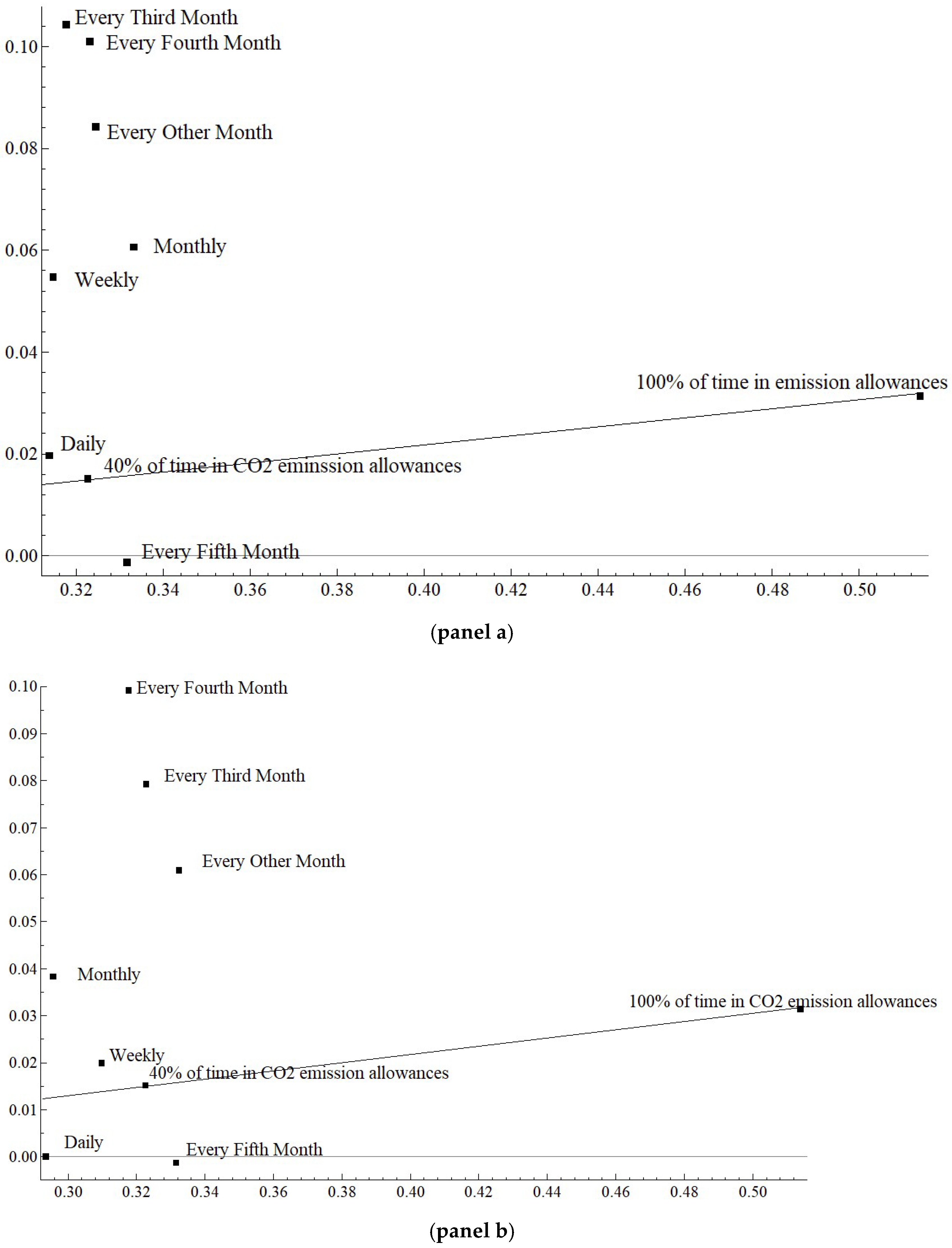
Figure 3 illustrates a clear negative stochastic trend from spring 2011 to spring 2013, and a clear positive stochastic trend from spring 2017 to fall 2018. Figure 4 (panels a and b) shows the results for a risk averse investor investing in CO₂ emissions allowances from 2 December 2008 to 28 September 2018. In the figure, the straight line depicts the theoretical efficient random timing return to the volatility frontier.

The black squares on the frontier line represent the returns to volatility performance for an investor who chooses randomly the dates to invest in EU carbon emissions and when to keep the assets in three-month Euribor. The square closer to the vertical axis means investing in emissions allowances for 1026 days (40% from 2564 days), and the square at the far end of the line means investing for all 2564 days. Thus, the frontier line is upward sloping in both panels.

The MA observations in Figure 4 are reported in Appendix A (

Table A1. Annualized daily returns of MA40–MA200, average returns and Sharpe ratios.

Stock	B&H	MA200	MA180	MA160	MA140	MA120	MA100	MA80	MA60	MA40	Average Returns	Sharpe Ratio
Carbon Emission Allowances	0.031	0.000	0.028	0.032	0.054	0.008	0.014	−0.012	0.014	0.039	0.020	0.07
Coal ARA	0.025	0.074	0.076	0.093	0.087	0.076	0.108	0.120	0.094	0.056	0.087	0.56
Brent Oil	0.051	0.025	0.041	0.022	0.017	0.008	0.011	0.030	0.029	−0.020	0.018	0.07
STOXX600 Renewable Energy	−0.028	0.081	0.105	0.090	0.063	0.066	0.079	0.064	0.058	0.045	0.072	0.30
STOXX600 Oil and Gas	0.030	−0.049	−0.043	−0.026	−0.011	−0.039	−0.043	−0.032	−0.032	−0.071	−0.039	−0.20

Note: All returns are before dividends. Stoxx 600 Europe Renewable Energy Index has the average annualized dividend of 0.003 and Stoxx 600 Europe Oil and Gas Index has the average annualized dividend of 0.039. In addition, the average annualized risk-free yield has been +0.004 in the tested period. The Sharpe ratios are calculated with dividends. This procedure is identical from Table A1, Table A2, Table A3, Table A4, Table A5, Table A6 and Table A7.

,

Table A2. Annualized daily (every fifth trading day) returns of MAW8–MAW40 (W = number of weeks), average returns and Sharpe ratios.

Stock	B&H	MAW40	MAW36	MAW32	MAW28	MAW24	MAW20	MAW16	MAW12	MAW8	Average Returns	Sharpe Ratio
Carbon Emission Allowances	0.031	0.038	0.056	0.088	0.081	0.062	0.036	0.048	0.030	0.053	0.055	0.16
Coal ARA	0.025	0.082	0.078	0.082	0.074	0.083	0.086	0.106	0.086	0.018	0.077	0.49
Brent Oil	0.051	0.045	0.040	0.036	0.011	0.014	0.023	0.050	0.059	0.047	0.036	0.15
STOXX600 Renewable Energy	−0.028	0.093	0.111	0.130	0.108	0.114	0.129	0.110	0.135	0.116	0.116	0.48
STOXX600 Oil and Gas	0.030	−0.046	−0.049	−0.032	−0.015	−0.016	−0.026	−0.035	−0.021	−0.040	−0.031	−0.13

,

Table A3. Annualized daily (every 22nd trading day) returns of MA2–MA10, average returns and Sharpe ratios.

Stock	B&H	MA10	MA9	MA8	MA7	MA6	MA5	MA4	MA3	MA2	Average Returns	Sharpe Ratio
Carbon Emission Allowances	0.031	0.020	0.040	0.055	0.037	0.047	0.033	0.092	0.114	0.107	0.061	0.17
Coal ARA	0.025	0.090	0.081	0.085	0.087	0.087	0.092	0.106	0.070	0.014	0.079	0.50
Brent Oil	0.051	0.040	0.027	0.046	0.053	0.050	0.061	0.067	0.096	0.085	0.058	0.26
STOXX600 Renewable Energy	−0.028	0.102	0.102	0.115	0.066	0.136	0.132	0.089	0.095	0.043	0.098	0.39
STOXX600 Oil and Gas	0.030	−0.045	−0.039	−0.011	−0.011	−0.021	0.017	−0.003	−0.011	−0.019	−0.016	−0.03

,

Table A4. Annualized daily (every other month) returns of MAD2–MAD5 (D = every other month, 5, 4, 3, 2, are the numbers of observations in the rolling window), average returns and Sharpe ratios.

Stock	B&H	MAD5	MAD4	MAD3	MAD2	Average Returns	Sharpe Ratio
Carbon Emission Allowances	0.031	0.061	0.063	0.118	0.095	0.084	0.25
Coal ARA	0.025	0.090	0.081	0.085	0.087	0.087	0.55
Brent Oil	0.051	0.011	−0.017	−0.015	0.007	−0.003	−0.03
STOXX600 Renewable Energy	−0.028	0.079	0.079	0.093	0.085	0.084	0.36
STOXX600 Oil and Gas	0.030	−0.045	−0.040	−0.017	−0.042	−0.036	−0.18

,

Table A5. Annualized daily (every third month) returns of MAT2–MAT4 (T = every third month, and 4, 3, 2, are the numbers of observations in the rolling window), average returns and Sharpe ratios.

Stock	B&H	MAT4	MAT3	MAT2	Average Returns	Sharpe Ratio
Carbon Emission Allowances	0.031	0.079	0.083	0.150	0.104	0.32
Coal ARA	0.025	0.070	0.055	−0.033	0.030	0.17
Brent Oil	0.051	0.013	−0.012	0.078	0.027	0.11
STOXX600 Renewable Energy	−0.028	0.100	0.066	0.073	0.079	0.34
STOXX600 Oil and Gas	0.030	−0.009	−0.008	0.008	−0.003	0.07

,

Table A6. Annualized daily (every fourth month) returns of MAQ2–MAQ3 (Q = every fourth month, 3, 2, are the numbers of observations in the rolling window), average returns and Sharpe ratios.

Stock	B&H	MAQ3	MAQ2	Average Returns	Sharpe Ratio
Carbon Emission Allowances	0.031	0.099	0.103	0.101	0.30
Coal ARA	0.025	0.053	0.037	0.045	0.29
Brent Oil	0.051	0.036	0.067	0.051	0.22
STOXX600 Renewable Energy	−0.028	0.056	0.066	0.061	0.24
STOXX600 Oil and Gas	0.030	−0.032	−0.027	−0.029	−0.11

,

Table A7. Annualized daily (every fifth month) returns of MAC2 (C = every fifth month, 2 is the numbers of observations in the rolling window), average returns and Sharpe ratios.

Stock	B&H	MAC2	Average Returns	Sharpe Ratio
Carbon Emission Allowances	0.031	−0.001	−0.001	−0.02
Coal ARA	0.025	0.048	0.048	0.31
Brent Oil	0.051	0.090	0.090	0.39
STOXX600 Renewable Energy	−0.028	−0.018	−0.018	−0.08
STOXX600 Oil and Gas	0.030	−0.037	−0.037	−0.18

,

Table A8. Annualized daily volatility of MA40–MA200, average annualized volatility.

Stock	B&H	MA200	MA180	MA160	MA140	MA120	MA100	MA80	MA60	MA40	Average
Carbon Emission Allowances	0.514	0.293	0.301	0.301	0.304	0.311	0.312	0.315	0.337	0.348	0.314
Coal ARA	0.214	0.147	0.148	0.147	0.147	0.147	0.147	0.151	0.153	0.157	0.149
Brent Oil	0.323	0.198	0.201	0.199	0.204	0.206	0.207	0.205	0.212	0.221	0.206
STOXX600 Renewable Energy	0.386	0.227	0.233	0.228	0.233	0.237	0.239	0.244	0.258	0.257	0.239
STOXX600 Oil and Gas	0.218	0.130	0.132	0.130	0.132	0.132	0.131	0.134	0.133	0.136	0.132

,

Table A9. Annualized daily (every fifth trading day) volatility of MAW8–MAW40 (W = number of weeks), average annualized volatility.

Stock	B&H	MAW40	MAW36	MAW32	MAW28	MAW24	MAW20	MAW16	MAW12	MAW8	Average
Carbon Emission Allowances	0.514	0.296	0.301	0.306	0.307	0.311	0.317	0.315	0.338	0.342	0.315
Coal ARA	0.214	0.147	0.146	0.148	0.148	0.147	0.146	0.146	0.150	0.155	0.148
Brent Oil	0.323	0.200	0.200	0.202	0.204	0.208	0.210	0.212	0.220	0.212	0.207
STOXX600 Renewable Energy	0.386	0.227	0.227	0.227	0.234	0.241	0.244	0.244	0.248	0.254	0.239
STOXX600 Oil and Gas	0.218	0.131	0.130	0.129	0.132	0.132	0.132	0.137	0.135	0.138	0.133

,

Table A10. Annualized daily (every 22nd trading day) volatility of MA2–MA10, average annualized volatility.

Stock	B&H	MA10	MA9	MA8	MA7	MA6	MA5	MA4	MA3	MA2	Average
Carbon Emission Allowances	0.514	0.310	0.316	0.329	0.327	0.324	0.332	0.355	0.354	0.353	0.333
Coal ARA	0.214	0.145	0.146	0.148	0.148	0.150	0.151	0.149	0.155	0.148	0.149
Brent Oil	0.323	0.200	0.203	0.206	0.210	0.214	0.212	0.220	0.208	0.219	0.210
STOXX600 Renewable Energy	0.386	0.234	0.234	0.223	0.230	0.242	0.243	0.241	0.259	0.253	0.240
STOXX600 Oil and Gas	0.218	0.138	0.140	0.132	0.132	0.133	0.137	0.138	0.136	0.140	0.136

,

Table A11. Annualized daily (every other month) volatility of MAD2–MAD5 (D = every other month, 5, 4, 3, 2, are the numbers of observations in rolling window), average annualized volatility.

Stock	B&H	MAD5	MAD4	MAD3	MAD2	Average
Carbon Emission Allowances	0.514	0.332	0.336	0.316	0.314	0.324
Coal ARA	0.214	0.146	0.149	0.153	0.160	0.152
Brent Oil	0.323	0.194	0.209	0.195	0.209	0.202
STOXX600 Renewable Energy	0.386	0.234	0.234	0.245	0.257	0.243
STOXX600 Oil and Gas	0.218	0.142	0.148	0.135	0.129	0.138

,

Table A12. Annualized daily (every third month) volatility of MAT2–MAT4 (T = every third month, and 4, 3, 2, are the numbers of observations in the rolling window), average annualized volatility.

Stock	B&H	MAT4	MAT3	MAT2	Average
Carbon Emission Allowances	0.514	0.323	0.348	0.283	0.318
Coal ARA	0.214	0.145	0.156	0.145	0.149
Brent Oil	0.323	0.198	0.213	0.227	0.213
STOXX600 Renewable Energy	0.386	0.234	0.248	0.234	0.239
STOXX600 Oil and Gas	0.218	0.136	0.140	0.125	0.134

,

Table A13. Annualized daily (every fourth month) volatility of MAQ2–MAQ3 (Q = every fourth month, and 3, 2, are the numbers of observations in the rolling window), average annualized volatility.

Stock	B&H	MAQ3	MAQ2	Average
Carbon Emission Allowances	0.514	0.318	0.328	0.323
Coal ARA	0.214	0.136	0.142	0.139
Brent Oil	0.323	0.196	0.226	0.211
STOXX600 Renewable Energy	0.386	0.233	0.253	0.243
STOXX600 Oil and Gas	0.218	0.153	0.167	0.160

and

Table A14. Annualized daily (every fifth month) volatility of MAC2 (C = every fifth month, and 2 is the number of observations in the rolling window), average annualized volatility.

Stock	B&H	MAC2	Average
Carbon Emission Allowances	0.514	0.332	0.332
Coal ARA	0.214	0.141	0.141
Brent Oil	0.323	0.221	0.221
STOXX600 Renewable Energy	0.386	0.242	0.242
STOXX600 Oil and Gas	0.218	0.139	0.139

) (Carbon Emission Allowances) as averages for every frequency. Panel a of the figure reveals that market timing with MA rules generally outperform random market timing: Daily, weekly, monthly, every other month, every third month and every fourth month rules beat random market timing, on average. However, the lowest frequency, every fifth month, fails to overcome the random timing frontier.

Panel b of Figure 4 shows the MA results when the last 200 trading days, the last 40 weekly observations, the last 10 monthly observations, the last five of every other month observations, the last four of every third month observations, the last three of every fourth month observations, and the last two of every fifth month observations, are used. From the panel, one can see that all but every fifth month and daily frequencies produce a better performance than does theoretical random timing.

The same conclusion about the daily frequency is made in Reference [4], who examined the performance of MA rules with DJIA stocks over the last 30 years. The analysis also finds that the largest rolling windows produce the best results, but the lower is the frequency, the higher are the daily returns. This also seems to be the case with EU CO₂ Emissions Allowances during the last 10 years.

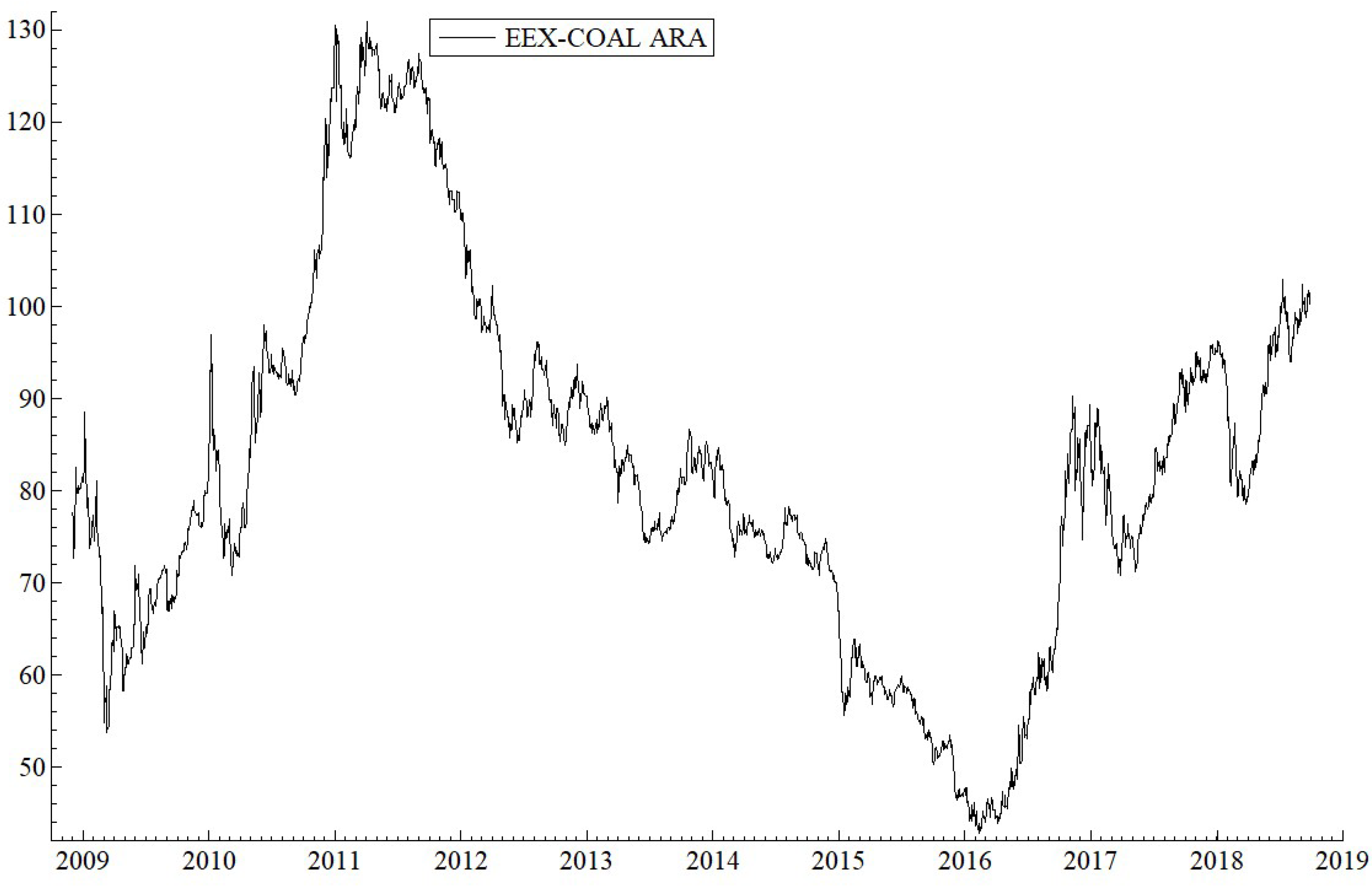
Figure 5 shows the development of EEX Coal ARA futures prices in USD per ton (API 2 CIF ARA; Argus-IHS McCloskey) from 2 December 2008 to 28 September 2018. The Coal ARA (Amsterdam-Rotterdam-Antwerpen) futures price can be seen as a fair reference price for a physical coal ton imported to Northwest Europe.

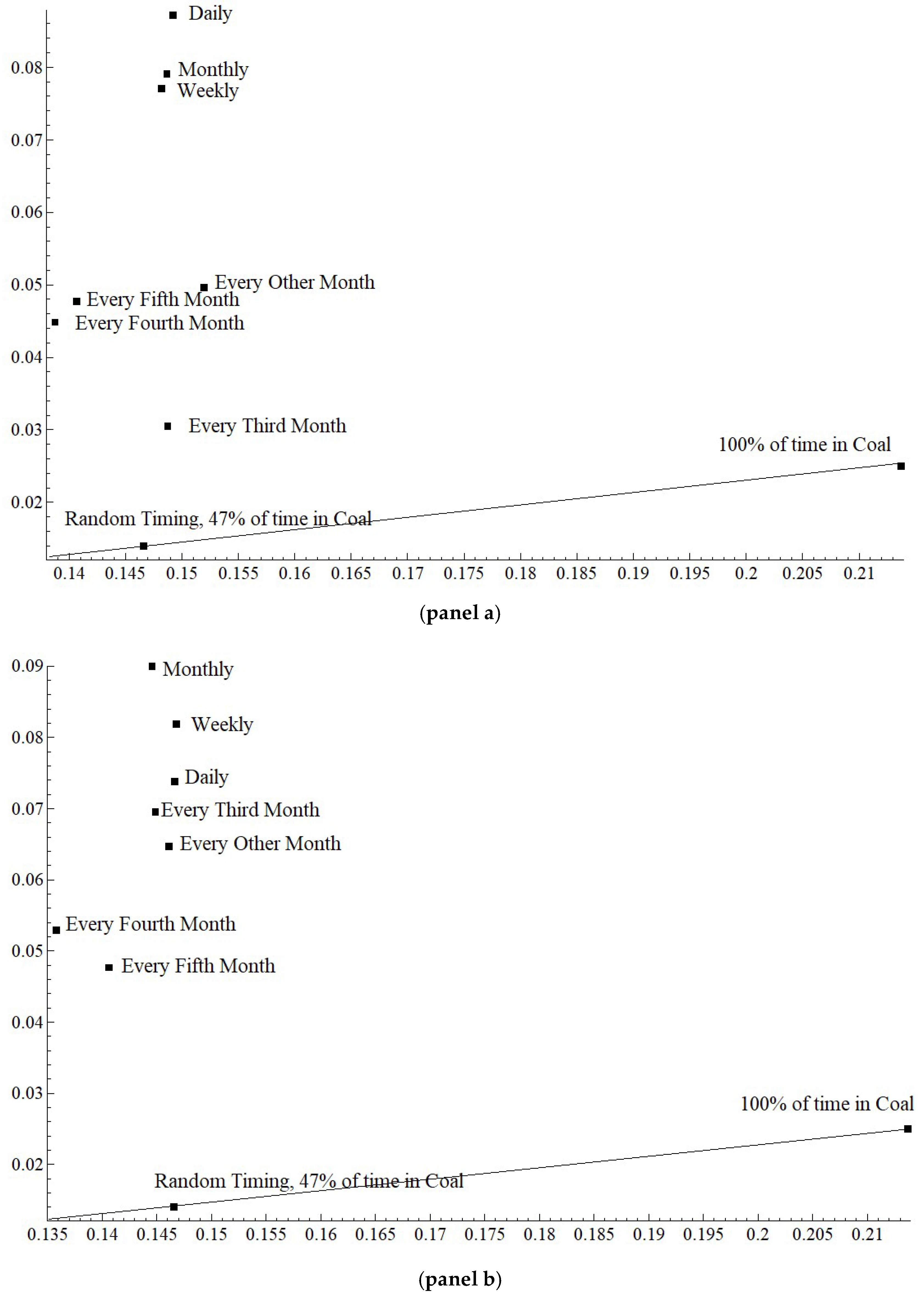
Figure 5 depicts an N-type curve: A positive stochastic trend from spring 2009 to spring 2011, followed by a negative stochastic trend to spring 2016, and again a positive trend to September 2018. Thus, the coal price series includes three significant stochastics trends within the period. Figure 6 (Panels a and b) plots the results for a risk averse investor investing in coal in Europe from 2 December 2008 to 28 September 2018. The black square on the random timing efficient frontier closer to the vertical axis represents the returns to volatility performance 47% of the time (that is, 1205 days) is randomly invested in coal and 53% of time in three-month Euribor.

In Figure 6, Panels a and b, the plot values are averages for every frequency, and come from the second rows of Appendix A (Table A1, Table A2, Table A3, Table A4, Table A5, Table A6, Table A7, Table A8, Table A9, Table A10, Table A11, Table A12, Table A13 and Table A14) (Coal ARA). Panel a of the figure shows that all MA market timing rules outperform random market timing. Therefore, European coal returns have been significantly predictable according to MA rules during the last 10 years. In contrast to the findings in Reference [4], it seems that the higher is the frequency, the better is the MA performance for coal returns.

Panel b of the figure shows the respective results when the outputs of all MA rules for all frequencies are calculated for only the largest rolling window sizes. The predictability of returns is also verified, as all MA rules outperform theoretical random timing. However, the plots are now more scattered in terms of frequencies, suggesting that the maximum window technique disposes of the above mentioned relation that the MA performance should depend positively on frequency.

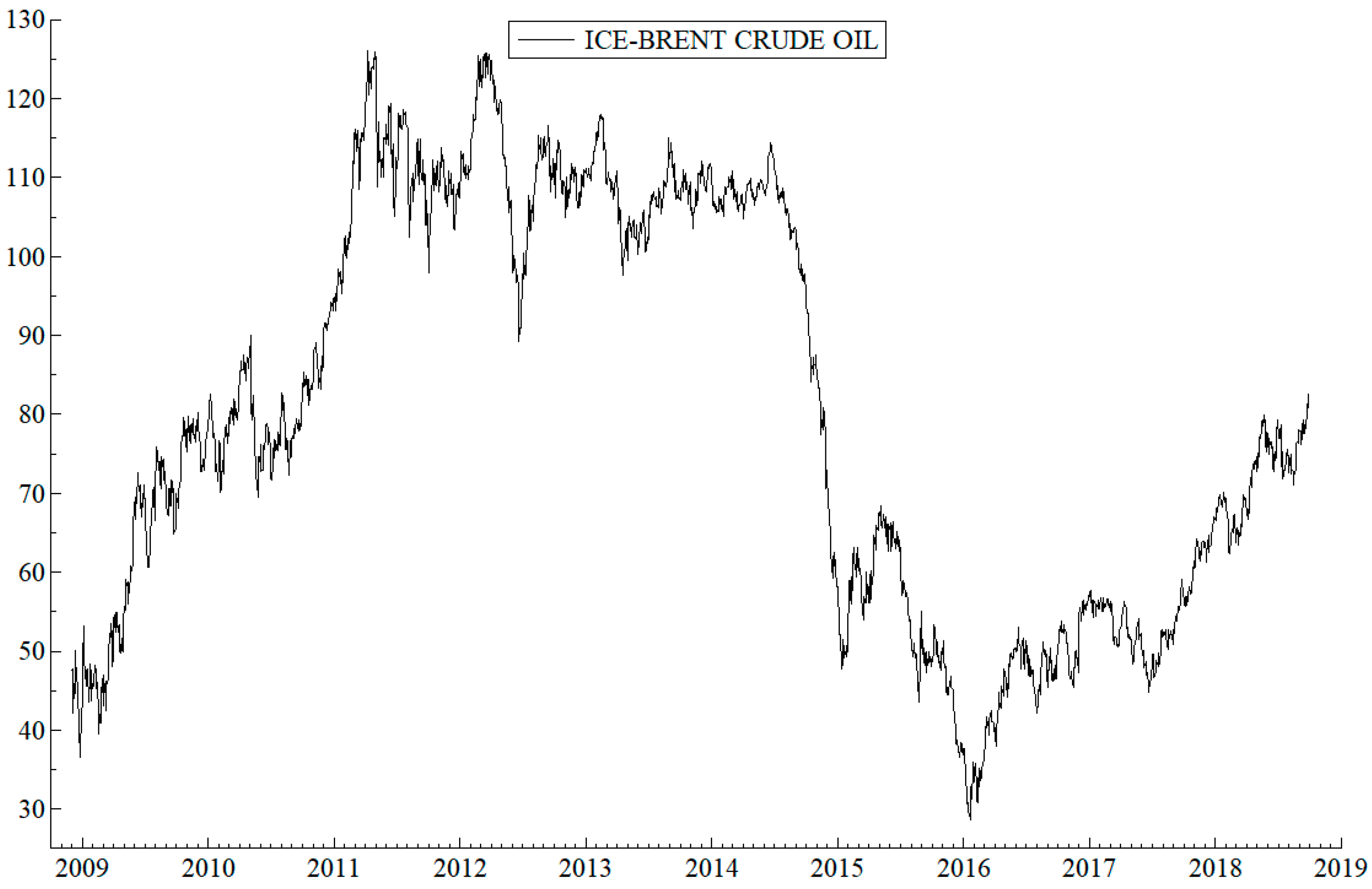
Figure 7 shows the observed daily future prices in ICE Brent Oil from 2 December 2008 to 28 September 2018. Figure 7 suggests that there is a positive stochastic trend from early 2009 to late 2011. Then, the prices stuck around 110 USD per barrel for four years, followed by a drastic drop in 2014, reaching as low as 30 USD in early 2016. Thereafter, there seems to be a positive trend until late September 2018. 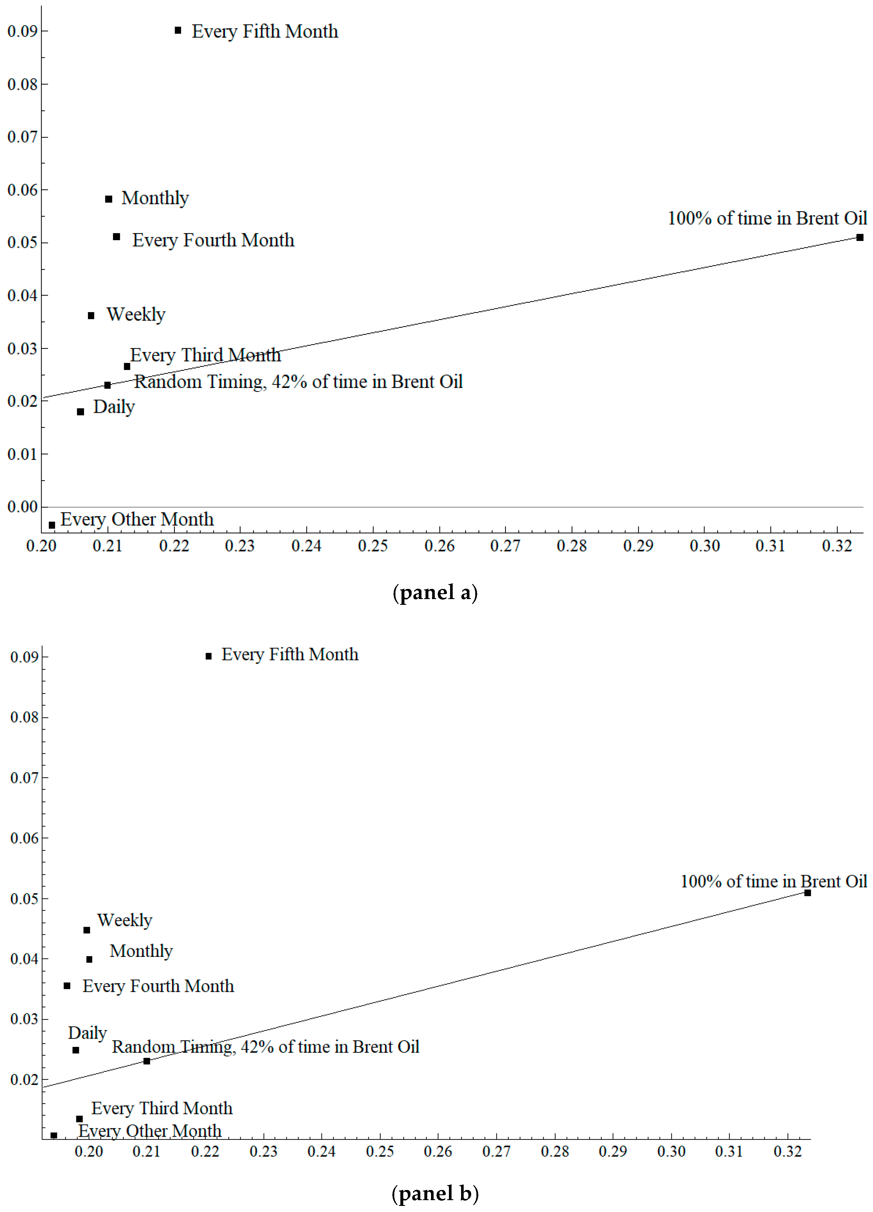Figure 8 (Panels a and b) shows the MA estimation results.

In Figure 8, five of the seven MA rules produce results above the random timing frontier in both panels. However, the frequency orderings differ between Panels a and b, in that the results do not clearly indicate returns predictability for Brent Oil futures over the last ten years. The MA plots in Figure 8 (averages for every frequency) are reported in the third rows in Appendix A (Table A1, Table A2, Table A3, Table A4, Table A5, Table A6, Table A7, Table A8, Table A9, Table A10, Table A11, Table A12, Table A13 and Table A14) (Brent Oil). It is possible that the absence of a stochastic trend from 2011 to 2014 mixes the results. Note that the results are significantly different for Coal and Brent Oil, even though both represent the primary fossil energy sources in Europe.

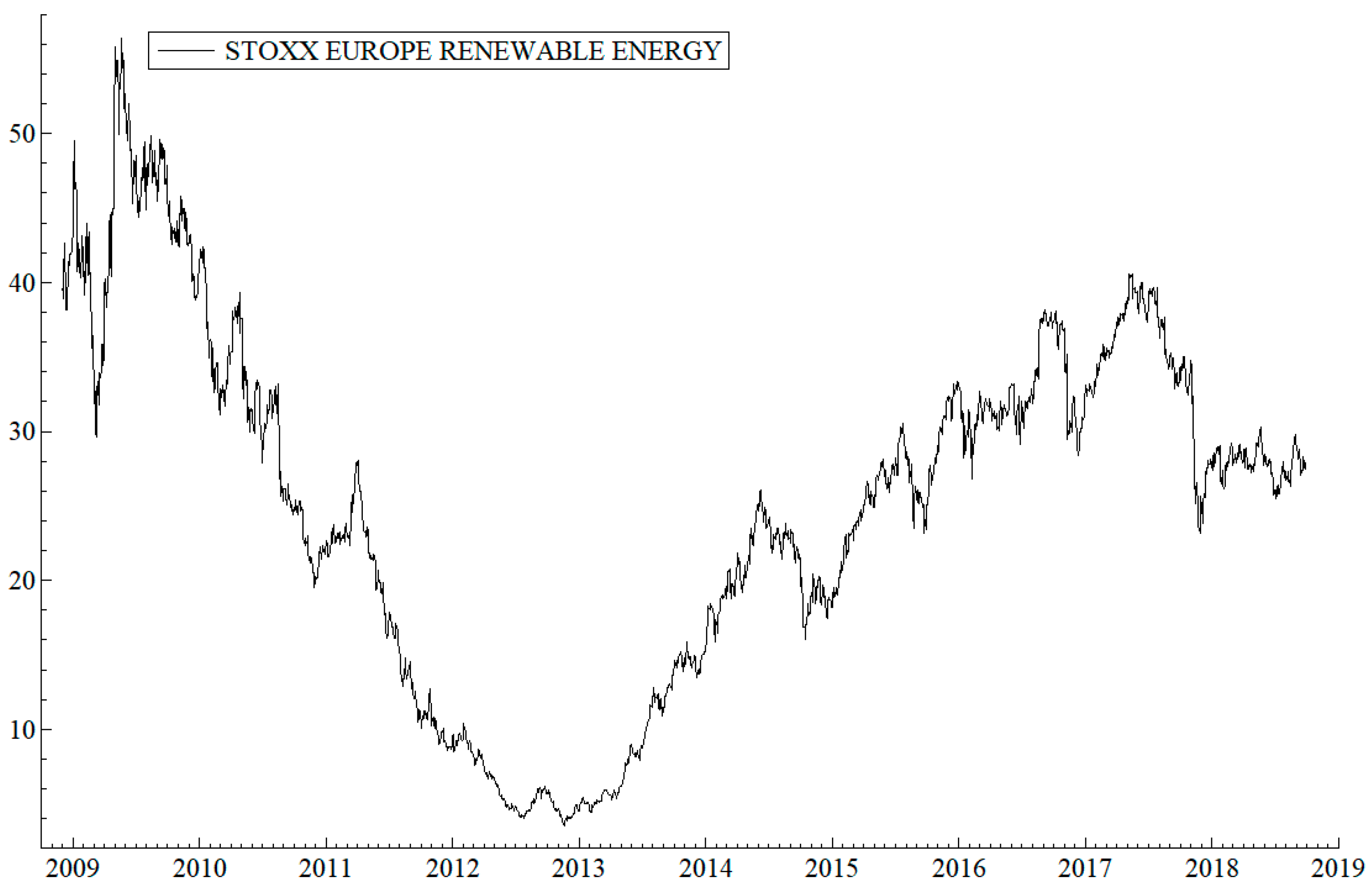
Figure 9 shows the observed daily prices for the Stoxx600 Europe Renewable Energy Index from 2 December 2008 to 28 September 2018.

Figure 9 reveals that the cumulative returns before dividends have actually been negative over the sample period. There is a visible negative stochastic trend (a drop from about 50 to 6 €) from spring 2009 to fall 2012, which is followed by a positive stochastic trend ending in spring 2017. The annualized dividends have been +0.003 for the period, resulting in negative total returns from 2 December 2008 to 28 September 2018. 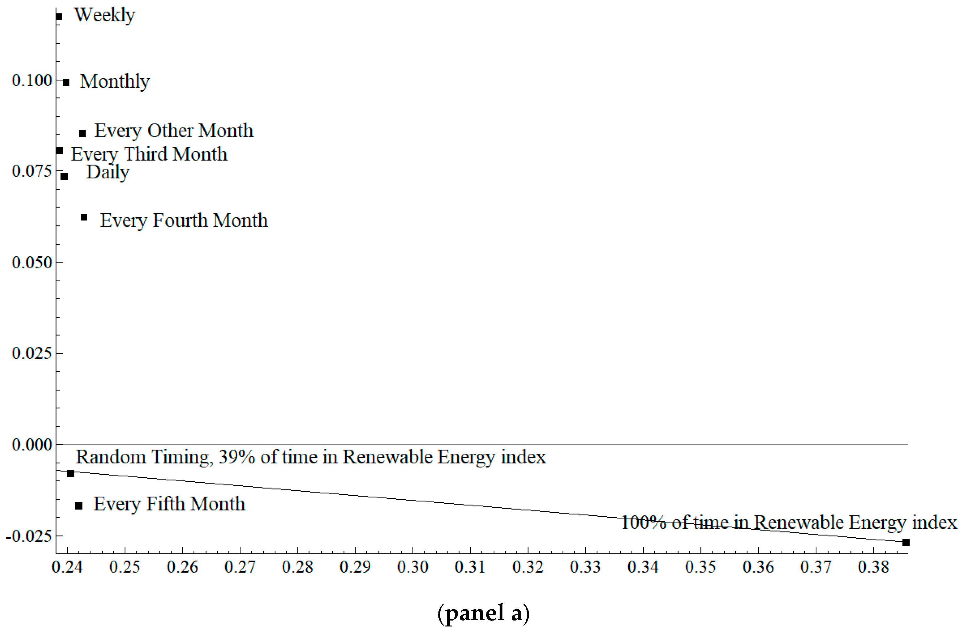Figure 10 confirms this by showing a downward sloping efficient random timing line, with 39% of the time invested in the Renewable Energy Index.

Figure 10 shows that, by random timing, positive returns to volatility ratio could have been achieved only by staying away from the index. The MA plots (averages for every frequency) are reported in the fourth rows in Appendix A (Table A1, Table A2, Table A3, Table A4, Table A5, Table A6, Table A7, Table A8, Table A9, Table A10, Table A11, Table A12, Table A13 and Table A14) (Renewable Energy Index). Panel a of the figure shows that all MA market timing rules outperform random market timing. Therefore, if a risk averse investor used market timing with MA rules, the investor would had earned about +0.070 returns with 0.24 volatility, on average.

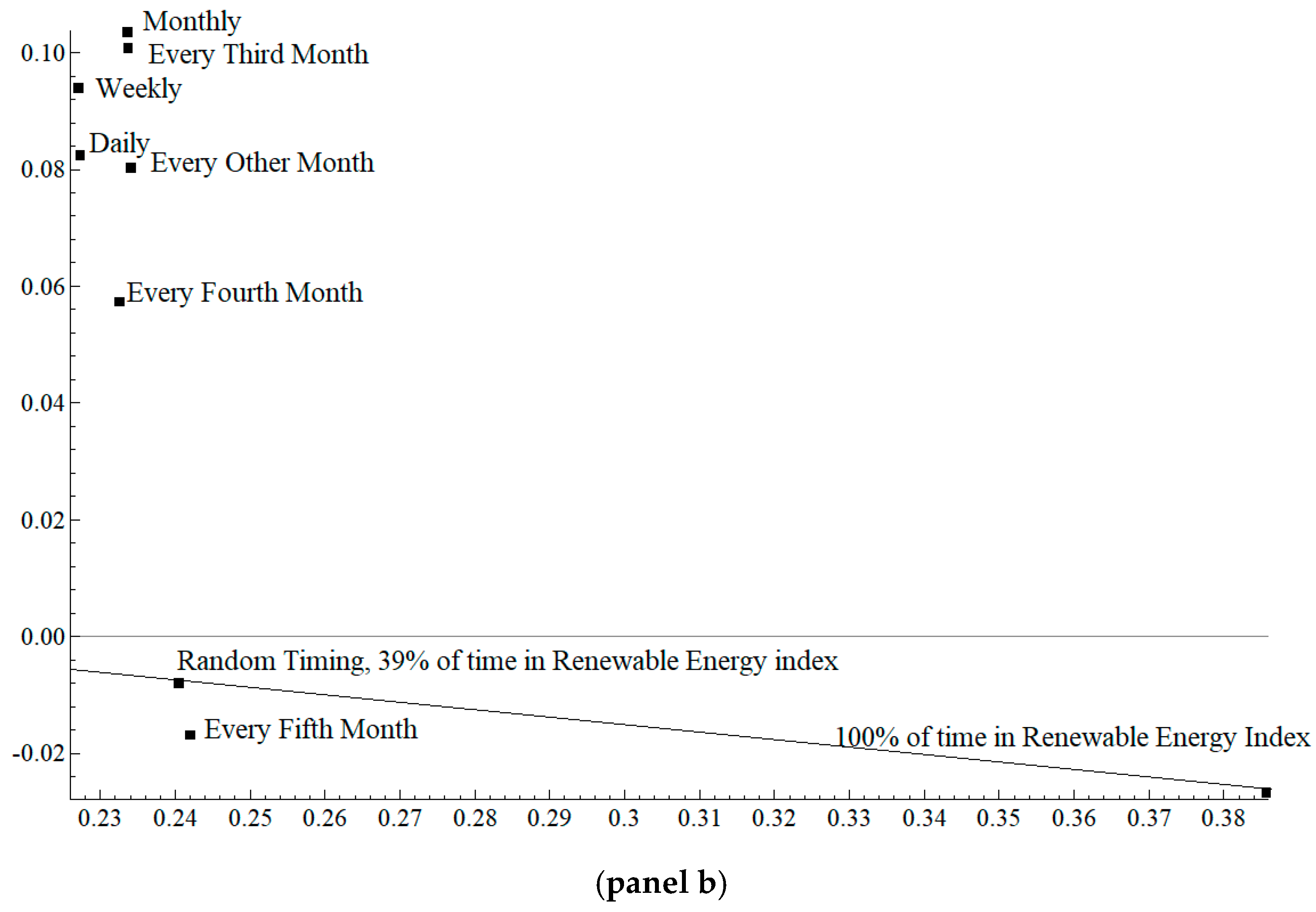
Panel b illustrates that if the whole rolling window size is used with the frequencies according to MA rules, the performance stays about the same as with narrower windows, resulting in an average Sharpe ratio of 0.31. Thus, the results illustrated in Figure 10 confirm that the returns have indeed been predictable for Stoxx 600 Renewable Energy index over the past 10 years.

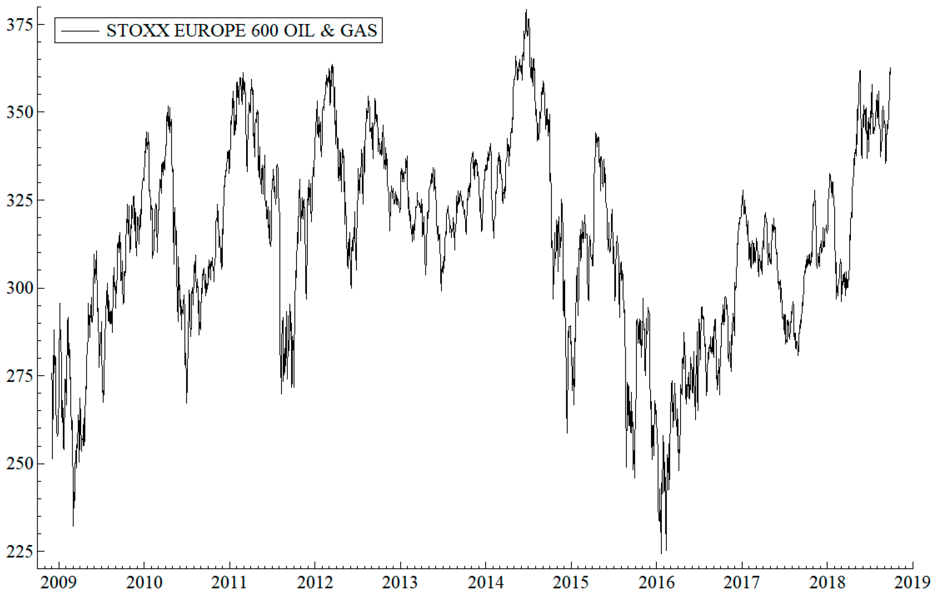
Figure 11 shows the development of European Oil and Gas Stock Index from 2 December 2008 to 28 September 2018.

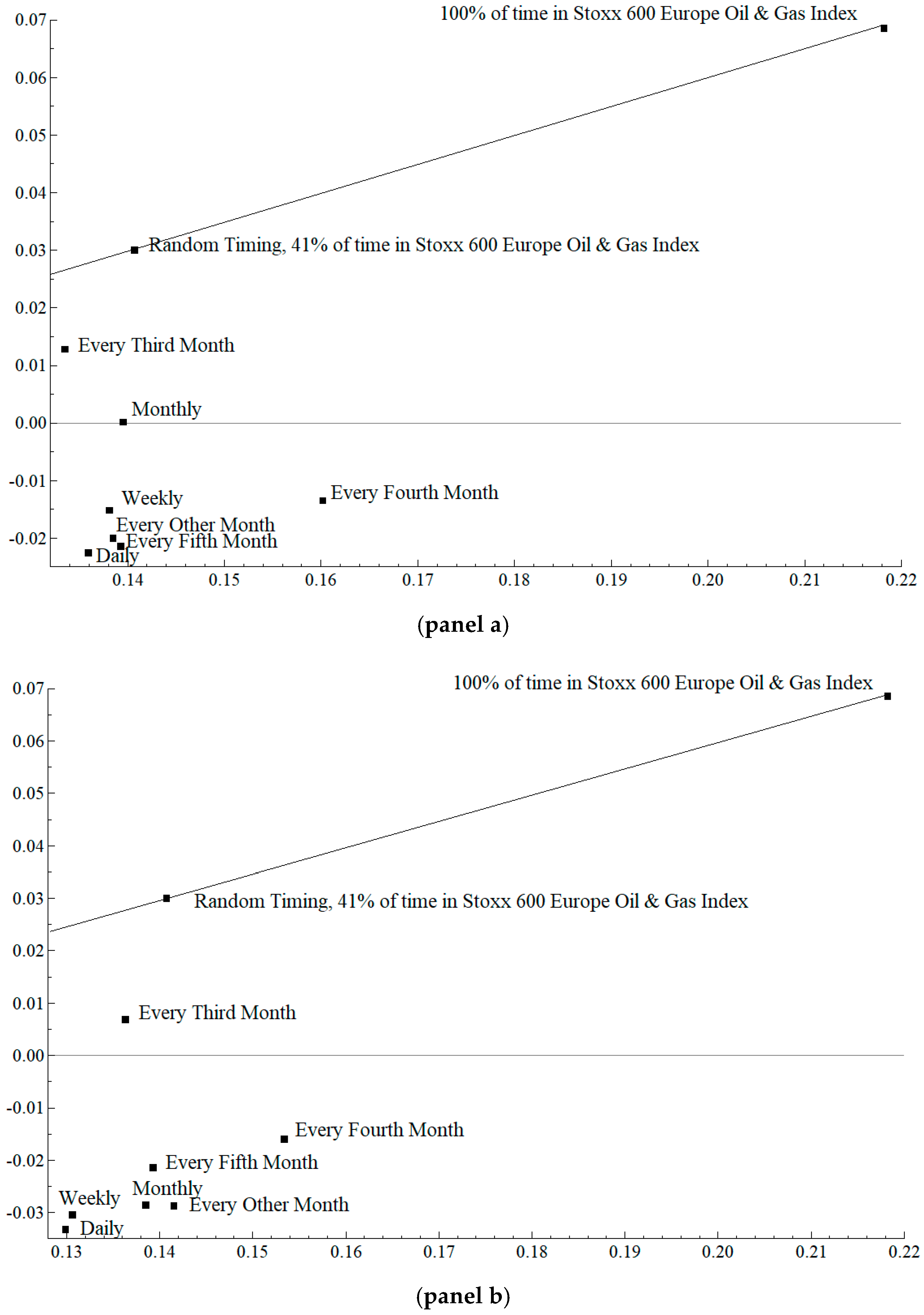
In Figure 11, on average, no clear lasting stochastic trends seem to exist in the development of the European Oil and Gas industry over the period. In addition, solid gains in stock prices and significant average annualized dividends have produced annualized returns of +0.070 with average volatility of 0.22 for the past 10 years. Figure 12, Panels a and b, reveals that, in the absence of stochastic trends in the index with solid total returns, random timing beats the MA rules in terms of returns to volatility performance.

The plots of Figure 12 are from the fifth rows in Appendix A (Table A1, Table A2, Table A3, Table A4, Table A5, Table A6, Table A7, Table A8, Table A9, Table A10, Table A11, Table A12, Table A13 and Table A14) (Oil and Gas Index). They show that all MA market timing rules significantly underperform random market timing. Note that random timing 41% of the time (1051 trading days) in Oil and Gas index produces +0.030, with volatility 0.14. In the figure, the relationship stays the same in both Panels. Therefore, the returns to volatility results with MA market timing rules confirm that there have been no predictable returns in the European oil and gas stocks over the last 10 years.

5. Concluding Remarks

We have tested returns predictability of EU CO₂ emission allowance prices over the last ten years, as well as the linked assets, namely EU Coal prices, Brent Oil prices, DJ Stoxx 600 Europe Renewable Energy Index, DJ Stoxx 600 Europe Oil and Gas Index, and EU Electricity one-day ahead future prices. We followed the literature by starting the sample data from the beginning of phase 2 of the EU ETS emission allowance allocations. The topic is important in light of the questionable capacity of the markets to control climate change, and because all the above subjects can be considered as financial assets traded in supposedly efficient markets. In efficient financial markets, market timing with Moving Average (MA) rules should not add value for risk averse investors, as compared with random market timing.

The empirical results are interesting for several reasons. First, we identified the data generating process in EU electricity prices as fractionally integrated (0.5), with a fractionally integrated GARCH process in the residual. This is a novel finding. The order of integration of order 0.5 implies that the process is not stationary but less non-stationary than the I(1) process, and that the process has long memory. This is probably because electricity cannot be stored. Returns predictability with MA rules requires stochastic trends in price series, indicating that the asset prices should obey the I(1) process, that is, to facilitate long run returns predictability. However, all the other price series tested in the paper are I(1)-processes, so that their returns series are stationary.

Second, we found that the EU Coal future price series creates significant returns predictability with MA rules, thereby adding value for a risk averse investor. The average annualized Sharpe ratio is 0.4, while 100% of time invested in coal produces a Sharpe ratio of 0.05. The results with EU CO₂ emission allowances are similar to those with coal, with the lowest frequency being an anomaly. This is an important finding since the literature has so far reported almost random walk behavior in daily data, indicating that market efficiency has improved as the sample size has grown. However, the results with Brent Oil prices are not as clear in this respect.

The European Renewable Energy stocks (DJ Stoxx 600 index) returns are significantly predictable with MA rules as all frequencies produce remarkably higher Sharpe ratios than does random timing. Moreover, the DJ Stoxx 600 Oil and Gas index does not produce returns predictability, and market timing with MA rules preforms poorly. The index has not developed long-lasting stochastic trends within the testing period. The average random timing Sharpe ratio is negative, but random timing produces positive Sharpe ratios, and 100% of the time in the index produces a Sharpe ratio of 0.30.

The empirical results are important because they corroborate the argument of Zhu and Zhou [42], and give a simple answer to the following question: When are MA rules useful? The answer is that, if significant stochastic trends develop in prices, long run returns are predictable, and market timing performs better than does random timing.