Numerical Study of Bubble Coalescence and Breakup in the Reactor Fuel Channel with a Vaned Grid

Abstract

The characteristics of bubbles of different sizes in fuel assembly are vital to two-phase flow resistance and heat transfer capacity. However, due to the swirl flow caused by the mixing vane, bubbles can crowd at the heated surface, which may anticipate the occurrence of departure from nucleation boiling. In the current work, the adiabatic two-phase flow in a simplified fuel assembly was analyzed by using the Eulerian two-fluid model and the MUSIG (MUltiple SIze Group) model. This computational domain consists of two coolant channels and two sets of vaned spacers, with three sets of periodic boundary conditions at the side faces of the domain. The distributions of vapor phase and bubble diameters were obtained, based on which the effects of mixing vanes on the bubble characteristics were analyzed. Vapor phase crowded at the rod surface in the higher inlet vapor fraction case, but crowded in the channel center in the lower inlet vapor fraction cases. This work can be used as a reference for the design of mixing vanes to avoid the anticipation of departure of nucleation boiling that may be caused by unreasonable design.

1. Introduction

Two-phase boiling flow has been widely used in power systems because of its high heat transfer performance compared with single-phase convective flow. In a newly designed pressurized water reactor (PWR), such as AP1000 (Westinghouse Co., Pittsburg, PA, USA), subcooled boiling and even saturated boiling is allowed in the core due to increasing confidence in the design and analysis technologies of PWR and the increasing demand on the economy of PWR. Under highly pressurized conditions, slight boiling in the reactor can significantly increase the heat transfer capability with no deterioration on the flow stability performance. However, the enhancement of the heat transfer ability is limited by the boiling crisis, where the wall heat flux reaches the critical heat flux and the local heat transfer coefficient decreases by one or two orders of magnitude. The wall temperature will increase dramatically by a hundred degrees under the condition where wall heat flux is specified, i.e., the cladding outer surface. Thus, the cladding and even the fuel pin may be burnt or melt, releasing vast radioactivity into the coolant.

Spacer grids and mixing vanes were placed in the fuel assembly to support the fuel rods and enhance the heat transfer capacity by generating the vortexes. However, as pointed by Krepper et al. [1] and Zhang et al. [2], bubbles will aggregate at parts of the rod surface due to the swirling caused by the mixing vane and that will lead to a vapor fraction peak at the rod surface, which may prevent the heat from being transferred to the liquid phase and result in the anticipation of the burnout. Thus, it is essential to investigate the vapor phase distributions for the two-phase flow in fuel assembly.

Two-phase flow has drawn lots of attention in the past few decades due to its essential role in the safety analysis of reactor systems. It has been studied by experimental and numerical methods traditionally, obtaining the basic senses on the two-phase nature and analysis tools such as RELAP-5, which are quite important to the design and safety analysis of nuclear reactor. However, these two traditional methods suffer from some critical defects. As for the experiments, it is a challenge to measure the localized parameters under high pressure and high temperature. Thermocouples, pressure sensors, mesh wires and even the laser technology can only measure one specified parameter from certain points or certain regions of the test section, and the whole field of multi-physics measurements are out of the question. Thus, it is difficult to detect the precise location of the hot spot on the cladding surface under the condition of a boiling crisis in the fuel assembly with vaned grid spacers. The traditional numerical methods, which mean the system codes and subchannel codes such as RELAP5 and COBRA, also suffer from these kinds of problems caused by the one-dimensional simplification. Even the three-dimensional version of such codes, such as RELAP5-3D and COBRA-TF, can solve the so-called spatially distributed thermohydraulics parameters, but it still solves the Euler equation on the coarse 3D meshes, rather than Navier-Stokes equations on fine meshes, and it cannot predict the spatial distribution of interested parameters in the coolant channel, which is critical for the safety of the reactor.

Several three-dimensional CFD models based on the two-phase Navier-Stokes equations were proposed to cope with the two-phase problems encountered in the nuclear power plants, including the two-fluid model [2,3], VOF (Volume of Fraction) model [4] and multi-field model [5]. The two-fluid model is most promising for engineering applications after an overall consideration on the accuracy and the computational cost and has been successfully used to predict localized two-phase flow characteristics [6]. In the two-fluid framework, bubble size is essential for the modeling of interactions between two phases. However, the bubble is poly-dispersed due to the breakup and coalescence, which itself is due to the swirling flow caused by the mixing vane. Thus, a model to consider the bubble size distribution is necessary for the modeling.

In this work, the two-fluid CFD methodology was employed to investigate the vapor distribution in the fuel assembly and on the rod surface, which might be related to the occurrence of CHF. The focuses of vapor distribution are the bubble size distribution and the aggregation of bubbles on the cladding surface. Thus, the adiabatic liquid-vapor two-phase flow in the fuel channel with spacer grid and mixing vane was simulated by the two-fluid framework coupled with the homogenous MUSIG (MUltiple SIze Group) model [7]. The characteristics of bubble breakup and coalescence were modeled. The effects of vaned spacer on the bubble diameter distribution mean bubble diameter and pressure drop were obtained.

2. Mathematical Models

As mentioned above, the Eulerian two-fluid framework for two-phase flow problem was employed to investigate the liquid-vapor flow. The mathematical models include Eulerian two-fluid model, phase interaction models and bubble size fraction model, i.e., the MUSIG model.

2.1. Eulerian Two-Fluid Model

There is no mass and heat transfer between the liquid and vapor phases for the adiabatic flow. The mass and momentum equations for liquid phase are given as:

$$\frac{\partial }{\partial t}({\alpha }_l{\rho }_l)+\nabla \cdot ({\alpha }_l{\rho }_l{U}_l)=0$$

(1)

$$\frac{\partial }{\partial t}({\alpha }_l{\rho }_l{U}_l)+\nabla \cdot ({\alpha }_l{\rho }_l{U}_l{U}_l)=-{\alpha }_{l}p+\nabla \cdot {\tau }_l+{\alpha }_l{\rho }_{l}g+F_{lg}$$

(2)

where α, $\rho$, U and $\tau$ denote the volume fraction, density, velocity and stress tensor for a specific phase, respectively; the subscript l means the liquid phase; g is the gravity; p is the pressure for both liquid and vapor phases, since these two phases share an equal pressure; F_lg is the interphase forces caused by the non-equilibrium between two phases, including the drag force, lift force, wall lubrication force, turbulent dispersion force and virtual mass force, i.e.,

$$F_{lg}=F_D+F_L+F_{WL}+F_{TD}+F_{VM}$$

(3)

where F_D, F_L, F_WL, F_TD and F_VM are the drag force, lift force, wall lubrication force, turbulent dispersion force and virtual mass force, respectively, which are defined in Section 2.3.

All these forces are calculated based on the local parameters in each computational cell, such as velocity, density and vapor fraction of each phase and the bubble diameter. These phasic parameters, except the bubble diameter, can be obtained by solving the two-phase governing equations. The bubble diameter is one of the key parameters in estimation of F_lg since all the interphase forces are calculated based on bubble diameter. However, the bubble diameter is not easy to determine due to the polydisperse characteristics of bubbles. The bubble size in a two-phase flow system may vary by one or two orders of magnitude, especially in a complicated geometry such as fuel assembly with mixing vanes. Many works were proposed to simplify the specification of bubble diameters in the two-phase CFD simulation. Thomas et al. [8] set the bubble diameters as a constant in the whole computation domain and tuned this value for different test conditions based on experience. Zhang et al. [3] and Krepper et al. [1] defined the bubble diameter as a function of localized fluid subcooling in each computational cell, which was better than Thomas et al.’s [8] work, but it still cannot present the polydisperse characteristics of bubble size. In the recent work on bubbly flow simulation, the bubble size distribution has been considered by using the PBM or the MUSIG models [9,10]. In the PBM and MUSIG models, bubble size fraction equations are solved along with a set of momentum equation for all of the gas phase. The bubble mean diameter, such as the Sauter mean diameter, is calculated based on the bubble size fraction and then used to solve the interphase transfer terms. These two models can deal with poly-dispersed bubbly flow with a limited range of bubble diameters. However, the direction of the interphase forces may change when bubble diameter exceeds a certain value, such as the lift force estimated by the Tomiyama model [11]. The method that averages bubble sizes to a single value cannot present different directions of interphase forces on bubbles with different sizes. The inhomogeneous MUSIG (iMUSIG) model was proposed to solve these problems with wide range of bubble diameters. Two sets of momentum equations were solved for small-diameter bubbles and large-diameter bubbles, respectively. The bubble diameters used in each momentum equation for the interphase actions were averaged from a set of bubble size fractions respectively. The diameter where lift force changes its sign is used as the critical value to divide the sets of bubble diameters. Thus, the governing equations for the poly-dispersed bubbles are given as follows:

$$\frac{\partial }{\partial t}({\alpha }_{g,i}{\rho }_g)+\nabla \cdot ({\alpha }_{g,i}{\rho }_g{U}_{g,i})=S_i$$

(4)

$$\frac{\partial }{\partial t}({\alpha }_{g,i}{\rho }_g{U}_{g,i})+\nabla \cdot ({\alpha }_{g,i}{\rho }_g{U}_{g,i}{U}_{g,i})=-{\alpha }_{g,i}p+\nabla \cdot {\tau }_{g,i}+{\alpha }_{g,i}{\rho }_{g}g+F_{gl,i}+M_i$$

(5)

where the subscript i means the bubble group. S_i and M_i are the mass source and momentum source caused by the bubble breakup and coalescence.

Due to the momentum conservation between liquid and vapor phases, the net interphase forces should be zero, i.e.,

$$F_{lg}=-{\displaystyle \sum _i{F}_{gl,i}}$$

(6)

As mentioned above, the iMUSIG model was proposed to deal with the two-phase flow with bubble size varying over a very large range exceeding the critical bubble size where lift force changes its direction. The homogeneous MUSIG model is qualified to model the bubble size distribution and its effects on the momentum transfer between two phases if most of the bubble sizes are lower than this critical size. It was found that size of most bubbles in the bubbly flow in fuel assembly with vaned spacers is lower than the critical value estimated by the Tomiyama model [11] after a series of simulation on the two-phase flow in fuel channels. Thus, in this work, the homogeneous MUSIG model was employed, and Equations (4)–(6) can be deduced into the following forms, i.e.,

$$\frac{\partial }{\partial t}({\alpha }_g{\rho }_g)+\nabla \cdot ({\alpha }_g{\rho }_g{U}_g)=0$$

(7)

$$\frac{\partial }{\partial t}({\alpha }_g{\rho }_g{U}_g)+\nabla \cdot ({\alpha }_g{\rho }_g{U}_g{U}_g)=-{\alpha }_{g}p+\nabla \cdot {\tau }_g+{\alpha }_g{\rho }_{g}g+F_{gl}$$

(8)

$$F_{lg}=-F_{gl}$$

(9)

2.2. MUSIG Model

The MUSIG model compiled in ANSYS CFX code is a framework based on the population balance model that can be used to handle the polydisperse bubbly flow with large size variation. Bubbles with different sizes are divided into several groups. The continuous bubble sizes are divided into several bins, each with a characteristic bubble size, i.e., $d_{g,i}$. The size fraction function (f_i) is used to present the fraction of bubbles located in each bin. Effects of bubble breakup and coalescence can be modeled by the fraction transfer among different bins. Thus, the governing equations for the size fraction function can be given as following equation:

$$\frac{\partial }{\partial t}({\rho }_g{\alpha }_g{f}_i)+\nabla \cdot ({\rho }_g{\alpha }_g{U}_g{f}_i)=S_{f,i}$$

(10)

where S_f,i is the source term of size fraction function for each group of bubbles, which is caused by the bubble breakup and coalescence and modeled by following equation:

$$S_{f,i}=B_{B,i}-D_{B,i}+B_{C,i}-D_{C,i}$$

(11)

where B_B,i and B_C,i are the birth rates due to larger bubble breakup and smaller bubble coalescence into group i; B_B,i and D_C,i are the death rates caused by the breakup into smaller bubbles and form into larger bubbles due to coalescence with other bubbles. These birth and death terms can be expressed as:

$$\{\begin{array}{l}{B}_{B,i}={\rho }_g{\alpha }_g({\displaystyle \sum _{j>i}g}(m_j:m_i)f_j)\hfill \\ D_{B,i}={\rho }_g{\alpha }_g({\displaystyle \sum _{j<i}g}(m_i:m_j))\hfill \\ B_{C,i}={({\rho }_g{\alpha }_g)}^2(\frac{1}{2}{\displaystyle \sum _{j\le i}{\displaystyle \sum _{k\le i}Q}}(m_j:m_k)X_{jki}{f}_j{f}_k\frac{m_j+m_k}{m_j{m}_k})\hfill \\ D_{C,i}={({\rho }_g{\alpha }_g)}^2({\displaystyle \sum _{j}Q}(m_i:m_j)f_i{f}_j\frac{1}{m_j})\hfill \end{array}$$

(12)

where m_i is the mass fraction of bubble size i. g(m_i:m_j) denotes the frequency of bubbles of size i breakup into bubbles of size j and the left part of the bubble. Q(m_i:m_j) represents the frequency of bubble coalescence between two bubbles from group i and j. X_jki is the coalescence mass matrix, defined by:

$$X_{jki}=\{\begin{array}{ll}\frac{(m_j+m_k)-m_{i-1}}{m_i-m_{i-1}}\hfill & \mathrm{if}{m}_{i-1}<m_j+m_k<m_i\hfill \\ \frac{m_{i+1}-(m_j+m_k)}{m_{i+1}-m_i}\hfill & \mathrm{if}{m}_i<m_j+m+k<m_{i+1}\hfill \\ 0\hfill & \mathrm{otherwise}\hfill \end{array}$$

(13)

The bubble breakup frequency g(m_i:m_j) is given by the Luo and Svendsen model [12], i.e.,

$$\mathrm{g}\left(m_i:m_j\right)=0.923F_B{\alpha }_l{\left(\frac{{\epsilon }_c}{d_i^2}\right)}^{1/3}{\displaystyle \underset{{\xi }_{\min }}{\overset{1}{\int }}\frac{{\left(1+\xi \right)}^2}{{\xi }^{11/3}}{e}^{-\chi }d\xi }$$

(14)

where

$${\xi }_{\min }=\frac{11.4{(\frac{{\nu }_l^3}{{\epsilon }_l})}^{1/4}}{d_i}$$

(15)

$$\chi =\frac{12\left({\left(\frac{m_j}{m_i}\right)}^{2/3}+{\left(1-\frac{m_j}{m_i}\right)}^{2/3}-1\right)\sigma }{\beta {\rho }_l{\epsilon }_l^{2/3}{d}_i^{5/3}{\xi }^{11/3}}$$

(16)

where ${\epsilon }_l$ and ${\nu }_l$ are the liquid phase eddy dissipation rate and kinematic viscosity, respectively. $\sigma$ is the surface tension.

The bubble coalescence frequency Q(m_i:m_j) is modeled by the Prince and Blanch model [13]; that is,

$$Q(m_i:m_j)=\left(F_T{S}_{ij}\sqrt{u_{ti}^2+u_{tj}^2}+F_B{S}_{ij}|U_{rj}-U_{ri}|\right)\cdot \exp \left(-{\left(\frac{{\rho }_l{r}_{ij}^3}{16\sigma }\right)}^{1/2}\ln \left(\frac{h_0}{h_f}\right)\frac{{\epsilon }_l^{1/3}}{r_{ij}^{2/3}}\right)$$

(17)

where

$$r_{ij}={\left(\frac{1}{2}\left(\frac{1}{r_i}+\frac{1}{r_j}\right)\right)}^{-1}$$

(18)

$$S_{ij}=\frac{\pi }{4}{(d_i+d_j)}^2$$

(19)

$$u_{ti}=\sqrt{2}{\epsilon }_l^{1/3}{d}_i^{1/3}$$

(20)

$$U_{ri}=\sqrt{\frac{2.14\sigma }{{\rho }_l{d}_i}+0.505g{d}_i}$$

(21)

2.3. Phasic Interaction Models

Momentum transfer can happen between the two phases due to the interphase non-equilibrium caused by the velocity difference and the gradients of velocity and vapor fraction. In this work, the drag force, lift force, wall lubrication force, turbulent dispersion force and virtual mass force are taken into consideration to model the adiabatic two-phase flow in the fuel assembly. The models are detailed in this section.

2.3.1. Drag Force

The drag force presents the resistance introduced by the relative velocity between bubbles and the surrounding liquid, acting in the opposite direction of the fluid flow and having a significant effect on the two-phase velocity fields. It is calculated by [7]:

$$F_D=\frac{3}{4}\frac{C_D}{d_g}{\alpha }_g{\rho }_l|U_g-U_l|(U_g-U_l)$$

(22)

where C_D is the drag force coefficient, estimated by the Ishii-Zuber correlation [14], considering of the bubbly flow with different bubbly sharps, i.e.,

$$C_D=\max (C_D(sphere),\min (C_D(ellipse),C_D(cap)))$$

(23)

where $C_D(sphere)$, $C_D(ellipse)$ and $C_D(cap)$ are the drag force coefficients for sphere bubble, ellipse bubble and cap bubble, respectively, defined by:

$$\{\begin{array}{l}{C}_D(sphere)=\frac{24}{R{e}_g}(1+0.15R{e}_g^{0.687})\hfill \\ C_D(ellipse)=\frac{2}{3}E{o}^{0.5}\hfill \\ C_D(cap)=\frac{8}{3}\hfill \end{array}$$

(24)

where the bubble Reynolds number (Re_g) and Eötvös Number (E_o) are defined by:

$$R{e}_g=\frac{{\rho }_l|U_g-U_l|d_g}{{\mu }_l}$$

(25)

and

$$Eo=\frac{({\rho }_l-{\rho }_g)g{d}_g^2}{\sigma }$$

(26)

where σ is the surface tension. dg means the Sauter mean diameter of bubble estimated by the bubble sizes (d_i) and bubble number density (n_i), which can be calculated from bubble size fraction. The Sauter mean diameter is calculated by:

$$d_g=\frac{{\displaystyle \sum _{i=1}^N{n}_i}{d}_i^3}{{\displaystyle \sum _{i=1}^N{n}_i}{d}_i^2}$$

(27)

2.3.2. Lift Force

The lift force represents the interphase actions on the bubbles caused by the liquid shear velocity field. This force is always orthogonal to the flow direction; that is, pointing to the wall or center of the channel. That means the lift force has a significant impact on the radial distribution of the vapor phase volume fraction. Lift force is calculated by [7]:

$$F_L=-C_L{\alpha }_g{\rho }_l(U_g-U_l)\times (\nabla \times U_l)$$

(28)

where C_L is the lift force coefficient and calculated by the Tomiyama correlation modified by Frank et al. [15].

$$C_L=\{\begin{array}{ll}\min (0.288\tanh (0.121R{e}_g),f(Eo\prime ))& Eo\prime \le 4\\ f(Eo\prime )& 4<Eo\prime \le 10\\ -0.27& Eo\prime >10\end{array}$$

(29)

where f(E_o′) is defined by:

$$f(Eo\prime )=0.00105{(Eo\prime )}^3-0.0159{(Eo\prime )}^2-0.0204Eo\prime +0.474$$

(30)

where E_o′ is a modified Eötvös number, defined by:

$$Eo\prime =\frac{({\rho }_l-{\rho }_g)g{d}_g^2{(1+0.163E{o}^{0.757})}^{2/3}}{\sigma }$$

(31)

2.3.3. Wall Lubrication Force

In the bubbly flow, small bubbles should be pushed to the wall since the lift force on small bubbles pointing towards the wall from fluid. However, it is observed that the bubbles are concentrated in the near wall region, but not immediately adjacent to the wall. It is because of the force acting on the dispersed bubble phase that push bubble away from the wall, named wall lubrication force, which is calculated by [7]:

$$F_{WL}=-C_{WL}{\alpha }_g{\rho }_l|U_g-U_l{|}^2{n}_W$$

(32)

where $n_W$ is the unit normal vector pointing away from the wall and C_WL is the wall lubrication force coefficient calculated by the Antal correlation [16]; that is,

$$C_{WL}=\max \left\{0,\frac{C_{W1}}{d_g}+\frac{C_{W2}}{y_W}\right\}$$

(33)

where y_W is the distance to the nearest wall from the cell center. The coefficients C_W1 and C_W2 are set as −0.01 and 0.05 respectively. It should be noted that the lubrication force only acts in a very thin layer next to the wall, with a cut-off distance of five time of Sauter diameter, beyond which the lubrication force will be zero.

2.3.4. Turbulent Dispersion Force

The distribution of bubbles dispersed in the liquid phase is affected by the turbulent eddies of liquid phase. The turbulent dispersion force is such a force to account the impacts of turbulent fluctuations of liquid velocity on the gas bubbles. It has a significant role in the radial vapor fraction and can be estimated by [7]:

$$F_{TD}=-C_{TD}{c}_{lg}\frac{{\mu }_{t,l}}{{\rho }_l{\sigma }_{lg}}\left(\frac{\nabla {\alpha }_g}{{\alpha }_g}-\frac{\nabla {\alpha }_l}{{\alpha }_l}\right)$$

(34)

where C_TD and σ_lg are coefficients, defined as 1.0 and 0.9, respectively [17]. μ_t,l is the turbulent viscosity of liquid phase; C_l,g is the momentum transfer coefficient caused by the interphase drag force, i.e.,

$$c_{lg}=\frac{3}{4}\frac{C_D}{d_g}{\alpha }_g{\rho }_l|U_g-U_l|$$

(35)

2.3.5. Virtual Mass Force

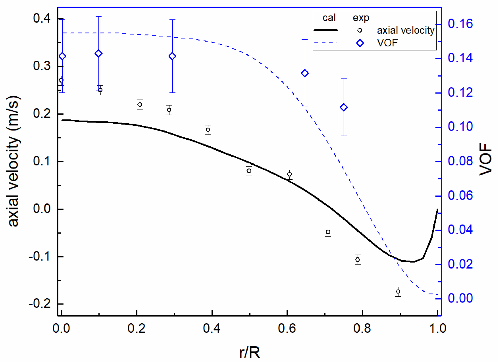
The virtual mass force will act on the bubble phase when bubble is accelerating relative to the continuous primary phase. This force is defined by [7]:

$$F_{VM}=-0.5{\alpha }_g{\rho }_l\left(\frac{\partial U_l}{\partial t}+(U_l\cdot \nabla )U_l-\left(\frac{\partial U_g}{\partial t}+(U_g\cdot \nabla )U_g\right)\right)$$

(36)

3. Model Validation

The experiments carried out by Vial et al. [18] were used as the benchmark to validate the models for two-phase flow. In their work, Laser Doppler technology was employed to measure the velocity and gas distribution in a bubble column. Gas was injected into a tube with 2 m length and 0.1 m diameter from a single orifice nozzle with 5 mm diameter at atmosphere pressure with gas injection velocity of 3.7 m/s. The profiles for velocity and gas volume fraction were measured in the downstream of the nozzle along the radial direction with uncertainties of ±15% and ±0.01 m/s, respectively. These data were used to validate current models. Only one-fourth of the fluid domain inside the tube was modeled given the symmetry of the geometry. Twenty groups of bubbles were set in the MUSIG model with initial bubble diameter of about 5 mm. The calculated vapor fraction and axial profiles were compared with experimental data in Figure 1. As can be seen, the predicted axial velocity agrees well with the experiment, generally. The gradient for predicted profile of axial velocity is slightly lower than that for experiment velocity profile, which might be because of the interfacial non-drag force, which is slightly related to the bubble shapes. Besides, it seems there is a slight increase for the axial velocity at the location of tube inner wall. Actually, it is a velocity decrease rather than a velocity increase. Reversed flow in the near wall region happens due to the concentrated vapor distribution in the tube center, which accelerates the two-phase mixture in the center of the channel and causes reverse flow in the near wall region. Thus, the axial velocity in the near wall region is negative. However, on the tube inner surface, the axial velocity is zero due to the non-slip boundary condition. Thus, it results in an increase in the profile of axial velocity near the wall. Besides, as can be noted, the predicted profile for vapor fraction locates in the uncertainties range of experiment data; while the predicted velocity profile doesn’t. As for the two-phase modelling, to predict the velocity profile is always more challenge than to predict the vapor fraction profile. It is because there are still some flaws in the models to mimic the interactions between the two phases, such the turbulent dispersion force and the lift force, which effects the velocity profile in the radial direction.

4. Two-Phase Flow in the Fuel Assembly with Two Channels

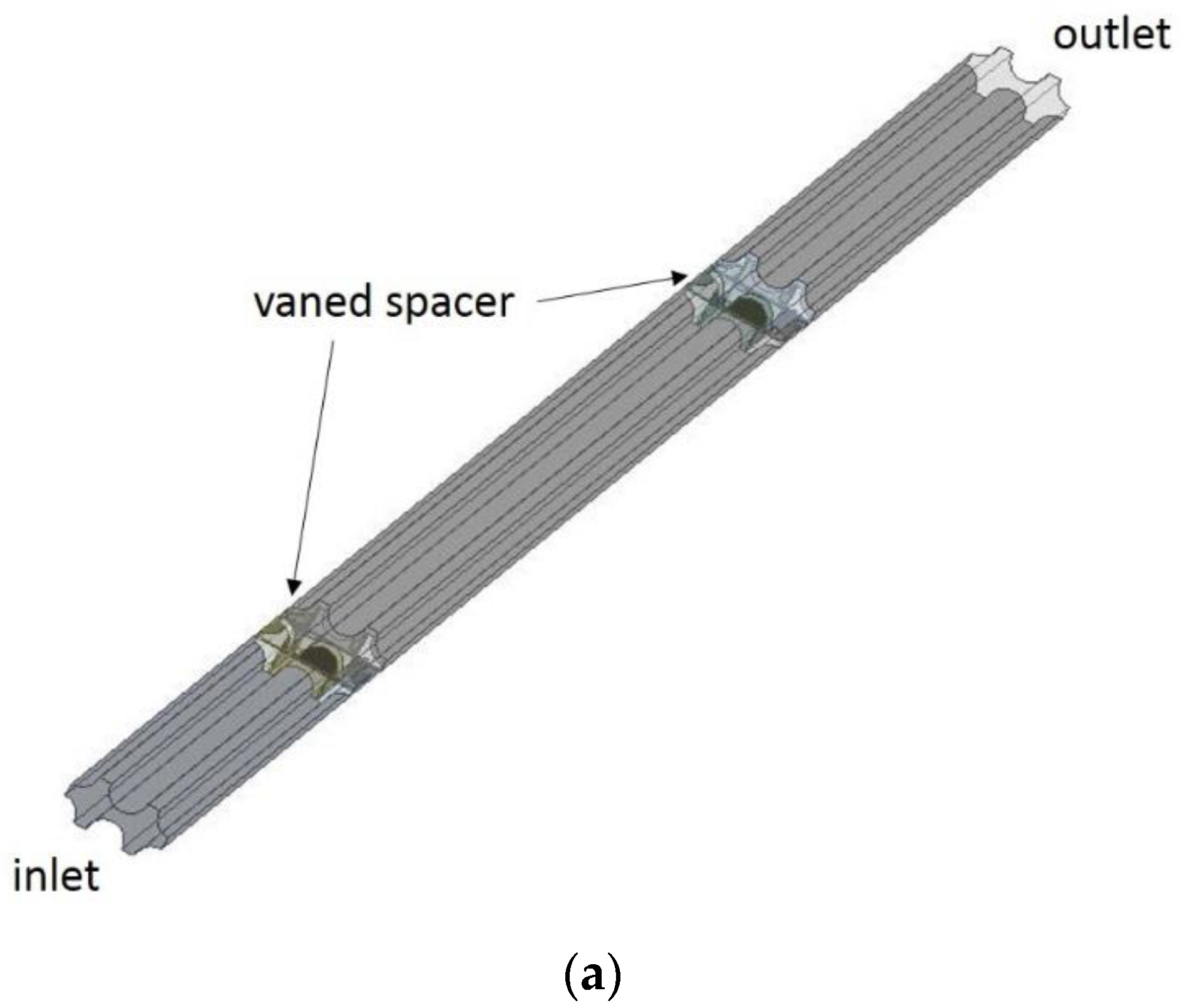
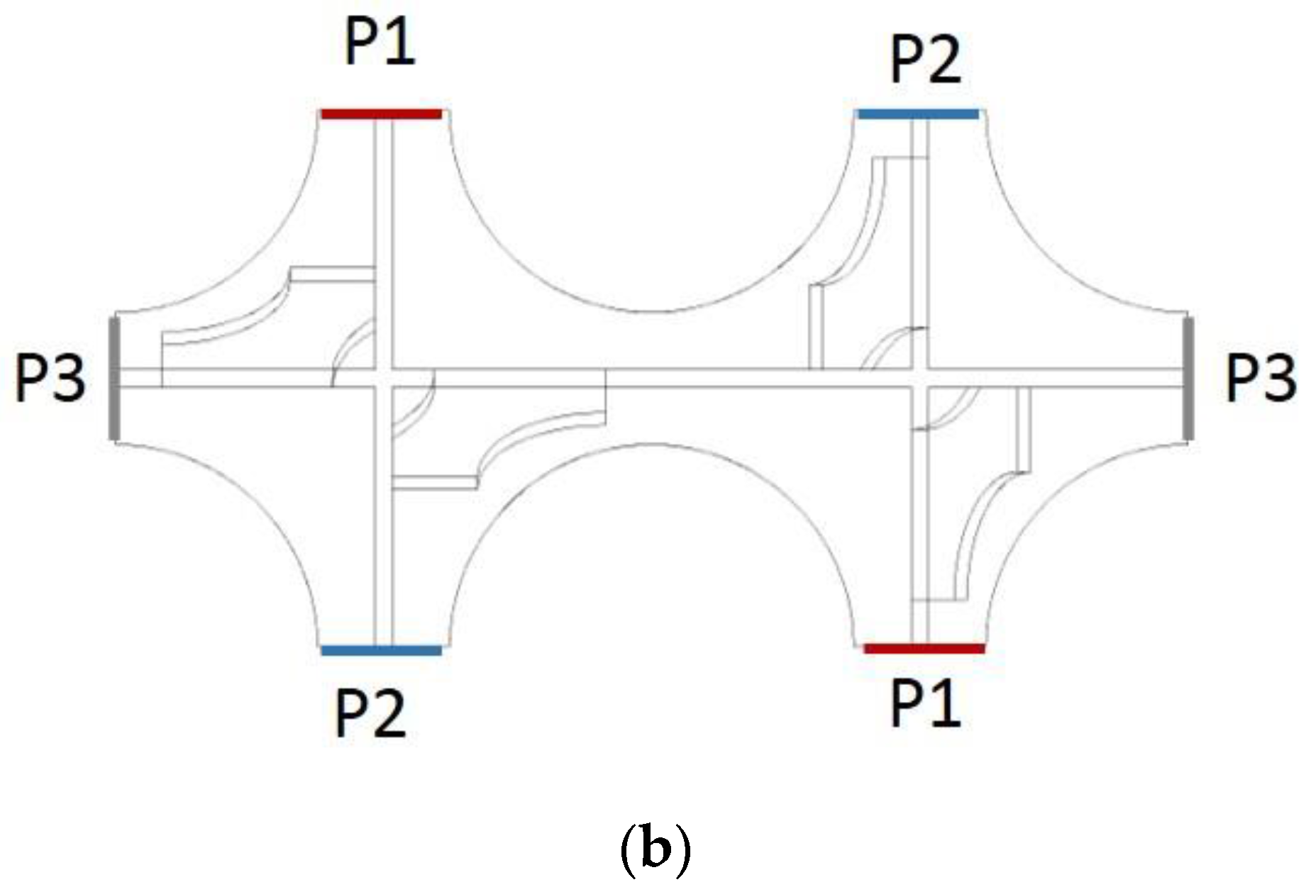
4.1. Geometry, Grid, Boundary Conditions and Numerical Scheme

In the typical reactor core, the reactor assembly comprises 17 by 17 fuel rods and about ten spacer grids. It requires too much computational cost to model the whole fuel assembly with 17 by 17 fuel rods, especially for two-phase in fuel assembly. In the past, researchers chose 5 by 5 fuel rods as a simplified geometry to study the single-phase and two-phase thermohydraulics by experiments and simulations. However, it still took up too many computational resources for the two-phase simulation in the assembly with 5 by 5 fuel rods with complicated physical models, such as the two-phase flow with MUSIG model. Fortunately, the arrangement of spacer grid and mixing vane shows some regularity and periodicity. In the work of Li and Gao [19], a two-channel model with three sets of periodic boundary conditions was proposed and compared with the results from a 5 by 5 rod geometry to prove the rationality of this simplification. This two-channel model was also employed in the current work for the purposes of reducing computational cost and obtaining reasonable results. The computational domain is shown in Figure 2. It consists of two channels, two sets of spacer grids and mixing vane. The cross-section connected to the adjacent channels is set to be periodic boundaries to allow the transverse flow to cross these boundaries. Besides, the weld bead as well as components to hold the bundles was omitted to simplify the modeling, since this work is focused on the effects of spacer grids and mixing vanes on thermohydraulics.

The computational domain was meshed by a mixing grid strategy, i.e., being divided into two kinds of subdomains, including the regions containing upstream and downstream of mixing vanes and the regions of mixing vanes. The upstream and downstream of mixing vanes were meshed by the swept hexahedral grids, while the subdomains of mixing vane vicinity were meshed by tetrahedral grids. These five subdomains are connected by interfaces with conformal grids to ensure the conservation at the interfaces.

As noted by Mahaffy et al. [20], mesh independence can be checked in two ways, i.e., increasing the grid quantity or increasing the solver precision. In the current research, two steps were taken to check the mesh independence. First, three sets of mesh strategies containing 0.92 M, 1.66 M, and 2.25 M cell elements were employed for simulation with single precision solver. The total pressure drop and outlet size fractions obtained from these three sets of meshes were compared and the results form mesh with 1.66 M elements shown almost no difference (less than 0.1%) with results from mesh with 2.25 M cells. After that, a double precision solver was employed to compare with single precision results based on the mesh with 1.66 M elements. No difference has been found between these two sets of results. Thus, the mesh strategy with 1.66 M cell elements was chosen as the independent one and used for further analysis.

Liquid-vapor two-phase mixture with a given vapor volume fraction flows into the inlet boundary with a uniform velocity profile of 5.0 m/s. Twenty sets of bubble sizes varying from 0.005 mm to 5 mm were employed to capture the size distribution of vapor phase. The bubble sizes are discretized by the geometric mass discretization method, i.e.,

$$d_i={\left(d_{\min }{}^3+0.75\frac{d_{\max }{}^3-d_{\min }{}^3}{2^{N-i}}\right)}^{1/3},i=1-N$$

(37)

where d_min and d_max are minimum and maximum bubble diameter limitations; N is the total number of bubble group.

All the governing equations are discretized by the high-resolution format and solved by CFX 17.1 code. Besides, the volume fraction was solved coupled with the velocity-pressure equations for a better convergence performance. The convergence criteria were set to be $1.0\times {10}^{-4}$ for all the variables.

4.2. Analysis on the Two-Phase Parameters in the Fuel Assembly

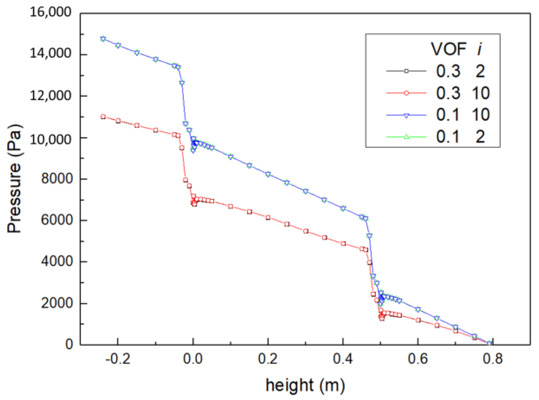
4.2.1. Cases Setup

In the two-phase flow with dense bubbles, two bubbles may coalesce if they collide with each other in the fluid domain under the actions of turbulence, eddy capture, velocity gradient or body force. Besides, large bubbles may break up due to forces from the surrounding liquid, such as the shear force caused by the liquid velocity gradient, the turbulence fluctuation and the interfacial slip. All these mechanisms on the breakup and coalescence are related to the density and the size of bubble. The baseline case was set with the inlet vapor fraction of 0.3 and all the bubbles in group 2; that is, the diameter of all the bubbles is 0.071 mm. Besides, three more cases were carried out as the control group to analyze the effects of inlet VOF and the inlet bubble diameter on the three-dimensional thermohydraulics parameters (

Table 1. Cases setup.

Case No.	Inlet VOF	Inlet Bubble Size
1	0.3	All in group 2
2	0.3	All in group 10
3	0.1	All in group 10
4	0.1	All in group 2

). The reference inlet VOF is 0.1 and the reference bubble diameter is 0.451 mm (all bubbles in group 10).

4.2.2. Results and Discussions

The results can be analyzed after reaching the convergence results for each case. All the cases were carried out with a transient solver strategy for better convergence performance. It will take about 50 h with 48 cores on a HPC for each case. First of all, the pressure drop characteristics along the flow channel are given in Figure 3. As can be seen, the initial bubble diameter makes no difference on the flow resistance for two-phase flow, while the vapor fraction makes a significant difference. Besides, most of the pressure drop in the channel was presented from the down surface of the spacer to the down surface of the mixing vanes. That means the main part of the pressure drop was a consequence of the flow area reduction at the low surface of spacer, rather than of the mixing vane.

The distribution of vapor fraction, which is crucial for heat transfer capacity at the rod surface, is shown in Figure 4, Figure 5 and Figure 6. Figure 4 and Figure 5 present the vapor fraction profiles at the planes downstream from the spacer with different distances for cases 1 and 4, respectively. As can be seen, there are significant differences between the results from these two cases. As for the first case with inlet vapor fraction of 0.3 (high vapor fraction case), there was obvious vapor crowding in the wake region of the transverse flow around the rod surface, especially at the plane 0.08 m from the spacer. Besides, a large amount of bubbles were aggregated at the center of the channel with vapor fraction lower than the vapor fraction near the rod surface. That means distinct bubble aggregation can be observed in the high vapor fraction case, which may lead to the departure from nucleation boiling (DNB) on the rod surface. When it comes to the low vapor fraction case, i.e., case 4 with inlet vapor fraction of 0.1, most of the bubbles aggregated at the center of channel, instead of the rod surface. Thus, there is no risk for the DNB in the low vapor fraction case. The vapor fraction distributions on the rod surface are also illustrated in Figure 6. In case 1, the vapor fraction at rod surface in the upstream of mixing vane was about 0.5. However, the vapor fractions on more of the rod surface in the downstream were much larger than 0.5, and can be as high as 0.9. In this case, the mixing vane would increase the vapor fraction at the wall, rather than decrease it, which is one of the purposes of the mixing vanes. On the other hand, the vapor fraction in the downstream region can be significantly reduced by the mixing vanes in the case of low inlet vapor fraction.

In addition to the vapor fraction, bubble diameters are also critical in the theory of bubble crowding for DNB. Figure 7 presented the diameter of the bubble at the plane of 0.08 m, which is the plane with maximum vapor fraction on the wall. As can be seen, for case 1, the bubble diameters near the rod surface and in the channel centers were about 0.35 mm. However, the bubble diameters in the channel centers for the low vapor fraction case were as high as 0.45 mm, which was because most of the bubbles were entrained into the center of the channels and coalesced into larger bubbles. Besides, the Sauter averaged diameter along the flow direction for each case was analyzed and is presented in Figure 8. It can be observed from this figure that the vapor fraction had obvious effects on the bubble diameter for the whole flow path, while inlet bubble diameter only made a big difference in the upstream of the first vaned spacer. After passing the first mixing vane, the Sauter diameters were almost the same for the cases with same inlet vapor fraction but different bubble size. That means the bubble breakup caused by the mixing vane will erase the effects of inlet bubble size. Furthermore, the strategy to investigate the bubble diameter characteristics by using only two sets of spacer grids was reasonable, since the parameters show periodic tendency after flowing pass the mixing vanes.

As mentioned in Section 2.3.2, the lift force was estimated by the Tomiyama model. However, as can be noted from Equation (29), the directions of lift forces for large and small bubble were not the same. That is, the bubbles can be pushed by the lift force towards the bulk or the wall, depending on the bubble diameter. Thus, there should be a critical value to divide these two sets of bubbles. For the current case with pressure of 15.5 MPa, this critical diameter was 2.1 mm. The bubbles larger or smaller than this critical diameter should be modeled by two sets of momentum equations, since they had different transverse velocity. However, in the current work, we use the homogenous MUSIG model with just one set of momentum equation, rather than the in-homogenous MUSIG model. This is because, according to our pre-analysis, most of the bubbles were smaller than 2.1 mm. Thus, we assumed that all the bubbles were in the smaller group of bubbles. Here, to validate the assumption, we calculated the fraction of each set of bubbles in Figure 9. In the upstream of the first spacer, about one-third of the vapor fraction located in the large group. However, the volume fractions of the large bubbles in the downstream of the mixing vane were rather small when compared with the fractions of small bubbles. Given the purpose of the current work (to investigate bubble information in the fuel assembly under the effects of vaned spacers), the MUSIG model was qualified for the current simulation.

In the downstream of the mixing vane, the bubbles break up due to the strong shear and turbulence caused by the mixing effects of the vanes. Then, the small bubbles may coalesce due to the collision of two adjacent bubbles under the actions of turbulence, eddy capture, velocity gradient, body force and wake. The process of bubble breakup and coalescence was a dynamic process, and even in that region a balance between breakup and coalescence was obtained. The dynamic evolution for each group of bubbles was investigated by analyzing the size fraction of bubbles. Figure 10 shows the size fractions of the bubbles in groups 2, 6, 8, 11 and 14 for cases 1 and 4, respectively. At the inlet of computational domain, all the bubbles were in group 2. Prior to the first vaned spacer, the fraction of group 2 decreased sharply to a low value of about zero. Meanwhile, a fraction of groups 6 and 8 increased right after flow into the computational domain. Then, group 11 became the dominated group with the largest size fraction for both of the two cases. In this period, the bubble coalescence was the dominating mechanism for the bubble evolution. After flowing past the vaned spacer, the fractions of larger bubbles (groups 11 and 14) dropped dramatically while fractions of moderately large bubbles (groups 6 and 8) increased immediately for case 1, due to the swirl flow caused by mixing vane. In this stage, the bubble breakup dominated. However, for case 4, only a fraction of group 6 increased sharply after the mixing vane, which means the bubbles after the breakup in the case of the larger inlet vapor fraction were larger than bubbles in the case of the lower inlet vapor fraction. In the region of about 0.2 m downstream of the mixing vane, bubbles coalesced again into larger bubbles in case 1, while this distance becomes about 0.3 m in case 4 with a lower inlet vapor fraction. The same phenomena can be observed in the region near the second spacer due to the periodicity of the geometry and the flow characteristics.

5. Conclusions

In the current work, the distribution of vapor phase in a simplified fuel assembly, which is related to the anticipation of critical heat flux, were investigated by a two-phase CFD code CFX with consideration of the characteristics of bubble coalescence and breakup. To model the two-phase flow with bubble size evolution, the Eulerian two-fluid model was employed with the interphase action models for momentum and turbulence transfer and the MUSIG model for bubble size evaluation. After validation, the models were used to simulate the two-phase flow in the assembly channel with periodic boundary conditions and two sets of vaned spacers. The following conclusions can be drawn from the results analysis.

(1)

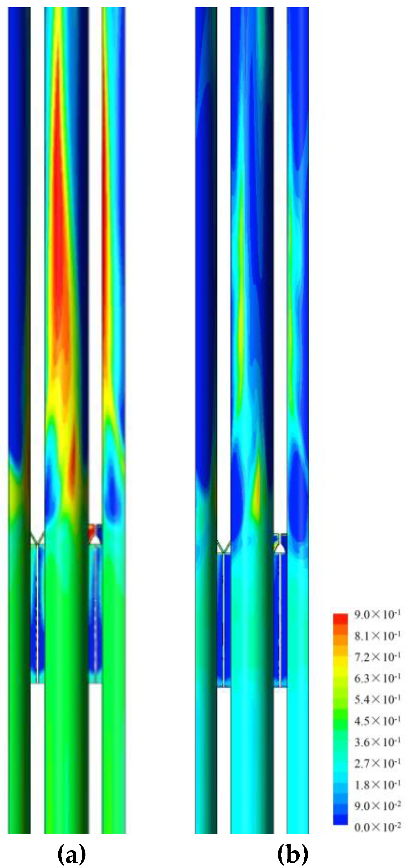
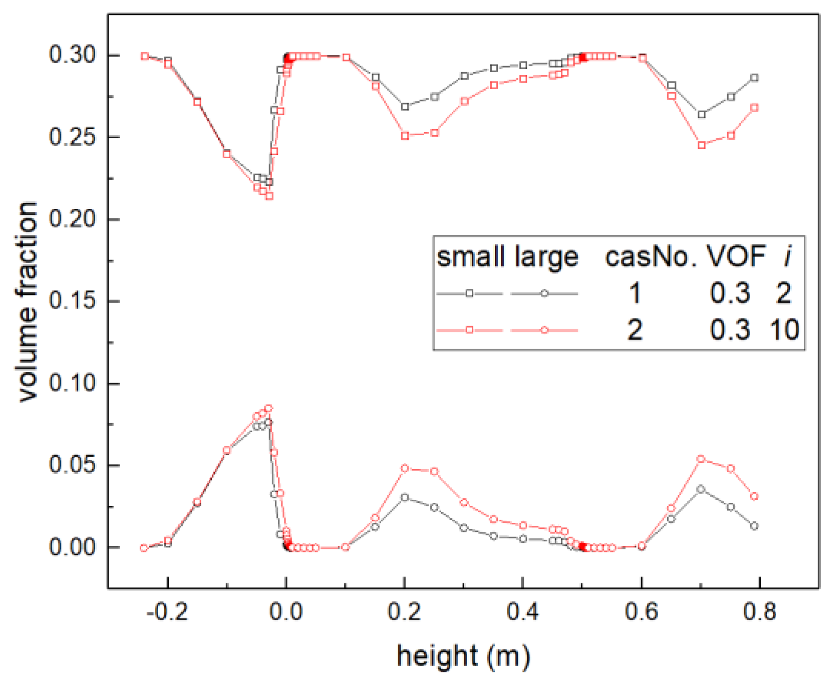
Vaned spacers caused sharp pressure drop, which is associated with the vapor volume fraction, rather than the inlet bubble size.

(2)

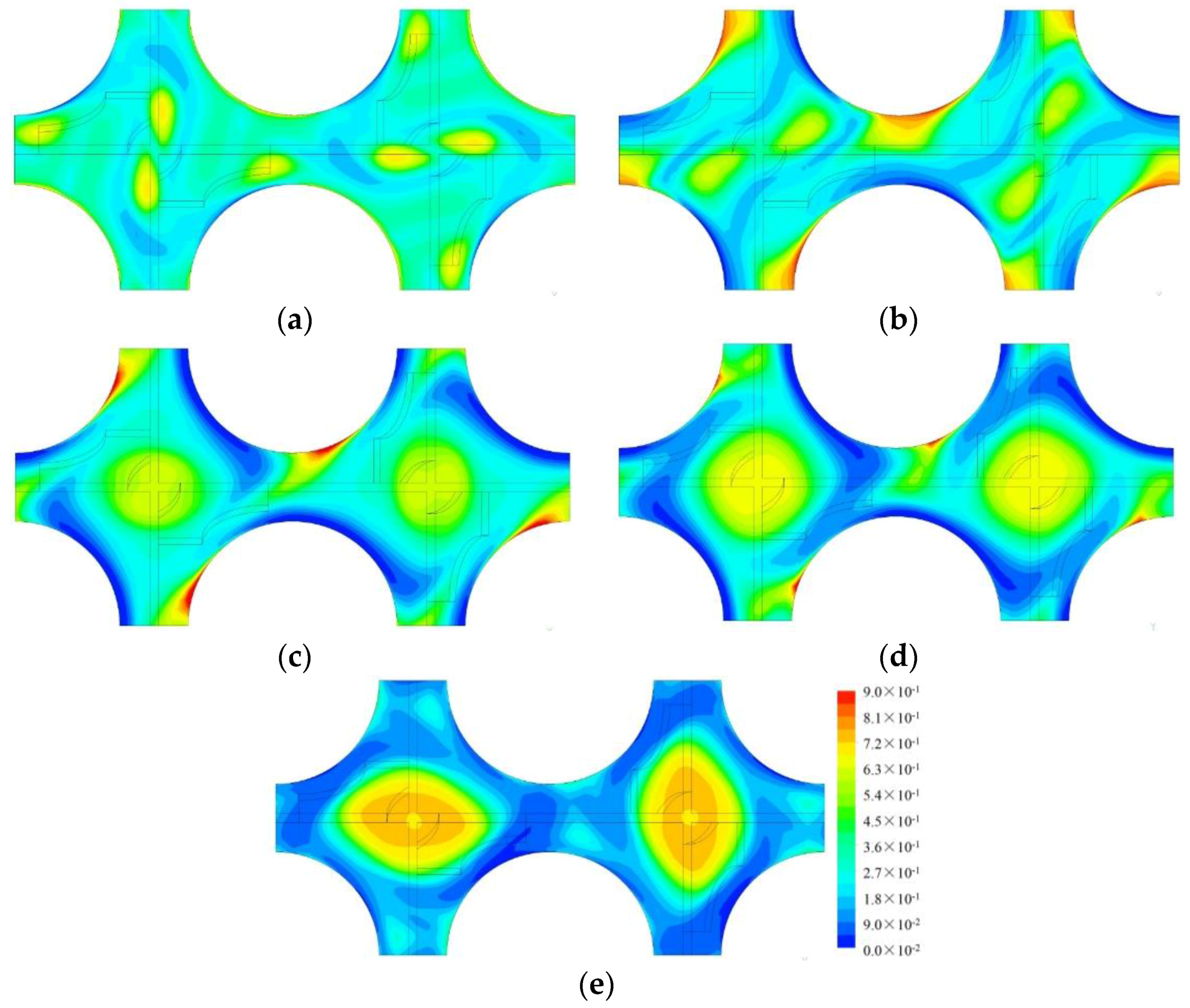
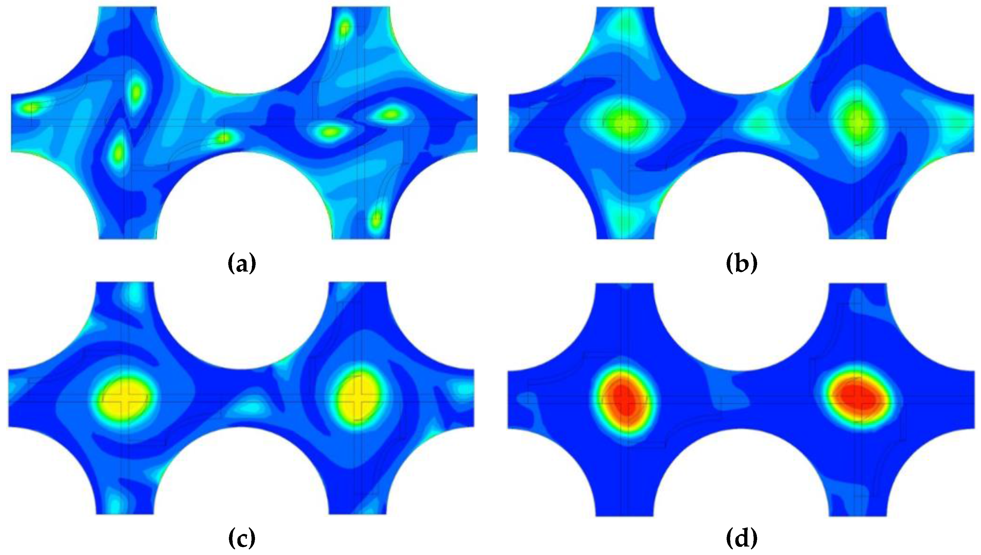
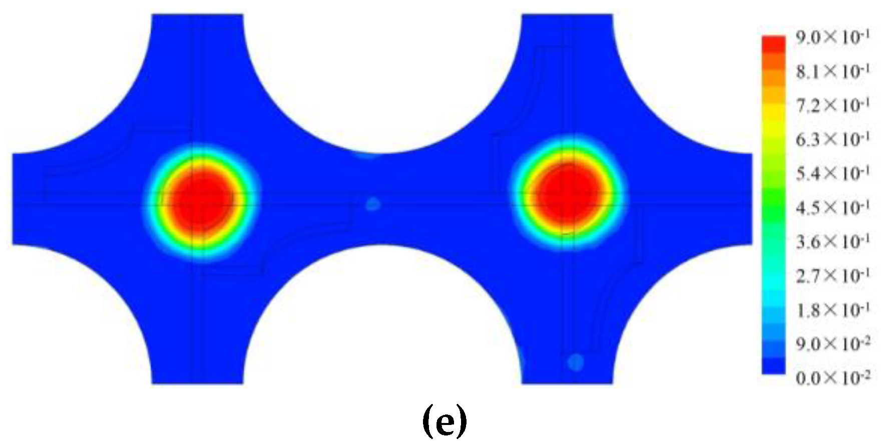
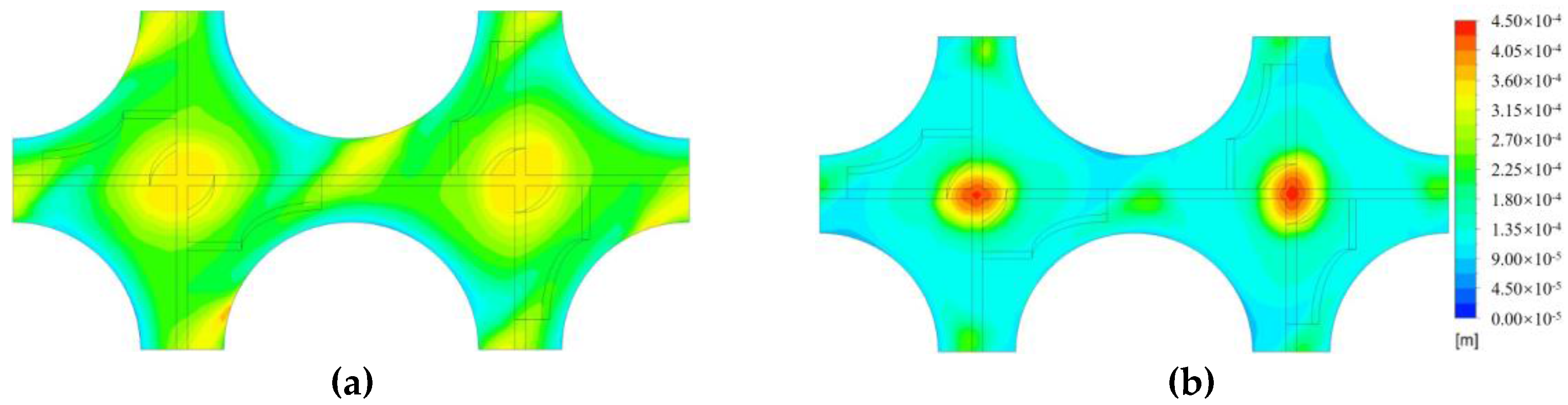
Vapor phase crowded at the rod surface for the higher inlet vapor fraction case, but crowded in the channel center for the lower inlet vapor fraction cases, i.e., increasing the inlet fraction can increase the risk of bubble aggregation at the rod surface, which might anticipate the critical heat flux under the condition of boiling two-phase flow.

(3)

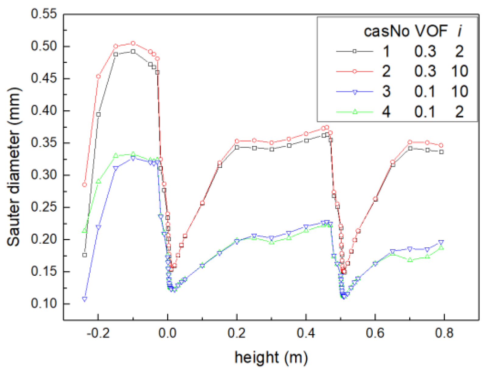
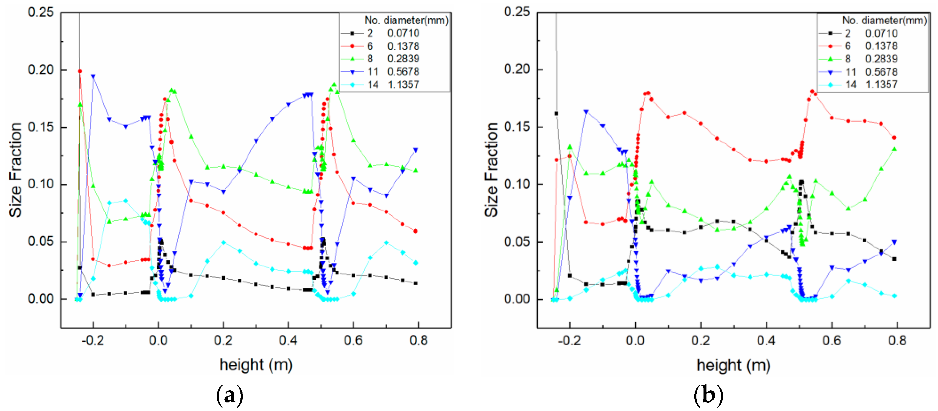
Mixing vanes can reduce the average bubble size by breakup. However, the bubble size distribution downstream of the mixing vane was related to the inlet vapor fraction, rather than the inlet bubble size.

References

1. Krepper, E.; Končar, B.; Egorov, Y. CFD modelling of subcooled boiling—Concept, validation and application to fuel assembly design. Nucl. Eng. Des. 2007, 237, 716–731. [Google Scholar] [CrossRef]
2. Zhang, R.; Cong, T.; Tian, W.; Qiu, S.; Su, G. CFD analysis on subcooled boiling phenomena in PWR coolant channel. Prog. Nucl. Energy 2015, 81, 254–263. [Google Scholar] [CrossRef]
3. Zhang, R.; Cong, T.; Tian, W.; Qiu, S.; Su, G. Effects of turbulence models on forced convection subcooled boiling in vertical pipe. Ann. Nucl. Energy 2015, 80, 293–302. [Google Scholar] [CrossRef]
4. Li, H.Y.; Yap, Y.F.; Lou, J.; Chai, J.C.; Shang, Z. Conjugate heat transfer in stratified two-fluid flows with a growing deposit layer. Appl. Therm. Eng. 2017, 113, 215–228. [Google Scholar] [CrossRef]
5. Liao, Y.; Rzehak, R.; Lucas, D.; Krepper, E. Baseline closure model for dispersed bubbly flow: Bubble coalescence and breakup. Chem. Eng. Sci. 2015, 122, 336–349. [Google Scholar] [CrossRef]
6. Bestion, D.; Anglart, H.; Mahaffy, J.; Lucas, D.; Song, C.-H.; Scheuerer, M.; Zigh, G.; Andreani, M.; Kasahara, F.; Heitsch, M.; et al. Extension of CFD Codes Application to Two-Phase Flow Safety Problems. Phase 2; NEA/CSNI/R(2010)2; OECD: Paris, France, 2010. [Google Scholar]
7. ANSYS Inc. ANSYS CFX-Solver Theory Guide, 14 ed.; ANSYS Inc.: Cononsburg, PA, USA, 2011. [Google Scholar]
8. Thomas, S.; Narayanan, C.; Lakehal, D.; Gong, Y. Multiphase Flow Simulation of Subcooled Boiling Using the N-Phase Approach in TransAT. In Proceedings of the 2013 21st International Conference on Nuclear Engineering, Chengdu, China, 29 July–2 August 2013; p. V003T10A015. [Google Scholar]
9. Lifante, C.; Reiterer, F.; Frank, T.; Burns, A. Coupling of wall boiling with discrete population balance model. J. Comput. Multiph. Flows 2012, 4, 287–298. [Google Scholar] [CrossRef]
10. Lucas, D.; Frank, T.; Lifante, C.; Zwart, P.; Burns, A. Extension of the inhomogeneous MUSIG model for bubble condensation. Nucl. Eng. Des. 2011, 241, 4359–4367. [Google Scholar] [CrossRef]
11. Tomiyama, A.; Tamai, H.; Zun, I.; Hosokawa, S. Transverse migration of single bubbles in simple shear flows. Chem. Eng. Sci. 2002, 57, 1849–1858. [Google Scholar] [CrossRef]
12. Luo, H.; Svendsen, H.F. Theoretical model for drop and bubble breakup in turbulent dispersions. AIChE J. 1996, 42, 1225–1233. [Google Scholar] [CrossRef]
13. Prince, M.J.; Blanch, H.W. Bubble coalescence and break-up in air-sparged bubble columns. AIChE J. 1990, 36, 1485–1499. [Google Scholar] [CrossRef]
14. Ishii, M.; Zuber, N. Drag coefficient and relative velocity in bubbly, droplet or particulate flows. AIChE J. 1979, 25, 843–855. [Google Scholar] [CrossRef]
15. Frank, T.; Shi, J.; Burns, A.D. Validation of Eulerian multiphase flow models for nuclear safety application. In Proceedings of the Third International Symposium on Two-Phase Modelling and Experimentation, Pisa, Italy, 22–25 September 2004. [Google Scholar]
16. Antal, S.; Lahey, R., Jr.; Flaherty, J. Analysis of phase distribution in fully developed laminar bubbly two-phase flow. Int. J. Multiph. Flow 1991, 17, 635–652. [Google Scholar] [CrossRef]
17. Burns, A.D.; Frank, T.; Hamill, I.; Shi, J.M. The favre averaged drag model for turbulent dispersion in Eulerian multi-phase flows. In Proceedings of the 5th International Conference on Multiphase Flow, Yokohama, Japan, 30 May–4 June 2004; JSME: Yokohama, Japan, 2004. [Google Scholar]
18. Vial, C.; Laine, R.; Poncin, S.; Midoux, N.; Wild, G. Influence of gas distribution and regime transitions on liquid velocity and turbulence in a 3-D bubble column. Chem. Eng. Sci. 2001, 56, 1085–1093. [Google Scholar] [CrossRef]
19. Li, X.; Gao, Y. Methods of simulating large-scale rod bundle and application to a 17 × 17 fuel assembly with mixing vane spacer grid. Nucl. Eng. Des. 2014, 267, 10–22. [Google Scholar] [CrossRef]
20. Mahaffy, J.; Chung, B.; Dubios, F.; Ducros, F.; Graffard, E.; Heitsch, M.; Henriksson, M.; Komen, E.; Moretti, F.; Morii, T.; et al. Best Practice Guidelines for the Use of CFD in Nuclear Reactor Safety Applications; NEA/CSNI/R(2007)5; OECD/NEA: Paris, France, 2007. [Google Scholar]
Figure 1. Comparison for the axial velocity and VOF.
Energies 11 00256 g001
Figure 2. Computational domain of the two-channel model. (a) sketch for the computational domain; (b) sketch for periodic boundary conditions.
Energies 11 00256 g002aEnergies 11 00256 g002b
Figure 3. Pressure drop along the flow direction.
Energies 11 00256 g003
Figure 4. Vapor fraction at downstream of vaned spacer for case 1: (a) L = 0.01 m, (b) L = 0.05 m, (c) L = 0.08 m, (d) L = 0.10 m, (e) L = 0.15 m (L is defined as the distance between the down surface of vane and the corresponding plane).
Energies 11 00256 g004
Figure 5. Vapor fraction at downstream of vaned spacer for case 4: (a) L = 0.01 m, (b) L = 0.05 m, (c) L = 0.08 m, (d) L = 0.10 m, (e) L = 0.15 m.
Energies 11 00256 g005aEnergies 11 00256 g005b
Figure 6. Vapor fraction on the rod surface: (a) case 1, (b) case 1.
Energies 11 00256 g006
Figure 7. Bubble diameter at the plane 0.08 m downstream from spacer: (a) case 1, (b) case 4.
Energies 11 00256 g007
Figure 8. Sauter averaged diameters along flow direction.
Energies 11 00256 g008
Figure 9. Volume fraction for large and small bubbles.
Energies 11 00256 g009
Figure 10. Size fraction for each group of bubbles: (a) Case 1, (b) Case 4.
Energies 11 00256 g010