CFD-Driven Valve Shape Optimization for Performance Improvement of a Micro Cross-Flow Turbine

Abstract

Turbines are critical parts in hydropower facilities, and the cross-flow turbine is one of the widely applied turbine designs in small- and micro-hydro facilities. Cross-flow turbines are relatively simple, flexible and less expensive, compared to other conventional hydro-turbines. However, the power generation efficiency of cross-flow turbines is not yet well optimized compared to conventional hydro-turbines. In this article, a Computational Fluid Dynamics (CFD)-driven design optimization approach is applied to one of the critical parts of the turbine, the valve. The valve controls the fluid flow, as well as determines the velocity and pressure magnitudes of the fluid jet leaving the nozzle region in the turbine. The Non-Uniform Rational B-Spline (NURBS) function is employed to generate construction points for the valve profile curve. Control points from the function that are highly sensitive to the output power are selected as optimization parameters, leading to the generation of construction points. Metamodel-assisted and metaheuristic optimization tools are used in the optimization. Optimized turbine designs from both optimization methods outperformed the original design with regard to performance of the turbine. Moreover, the metamodel-assisted optimization approach reduced the computational cost, compared to its counterpart.

1. Introduction

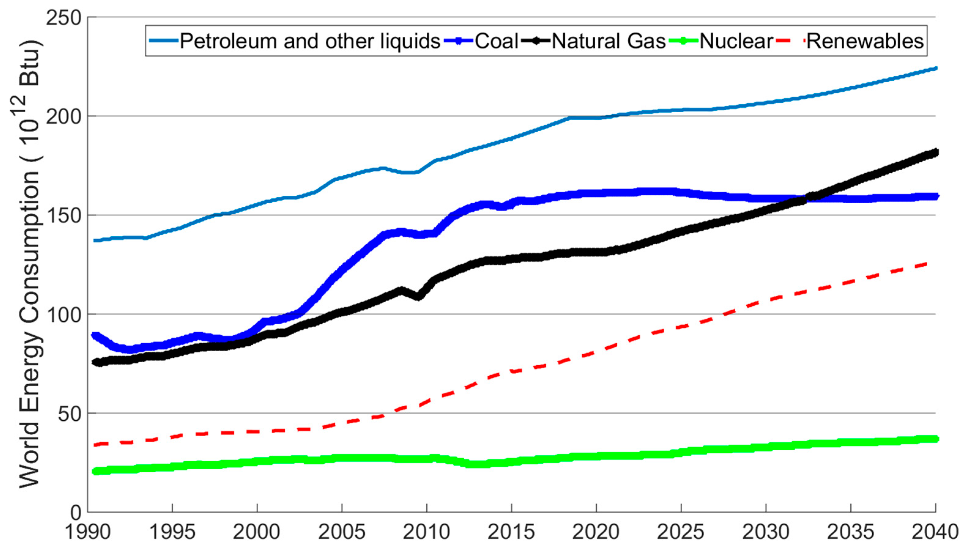
Due to the dynamically increasing population, competitive market economy and modernization, the global demand for energy is increasing dramatically. Projections from various studies indicate a large increase in energy consumption in the coming decades, especially in developing countries [1]. In the last two decades, the increased consumption of renewable energy sources has shown a surge (Figure 1). In fact, the studies project that this trend will also continue in the future. Among others, hydropower is the major source of renewable energy.

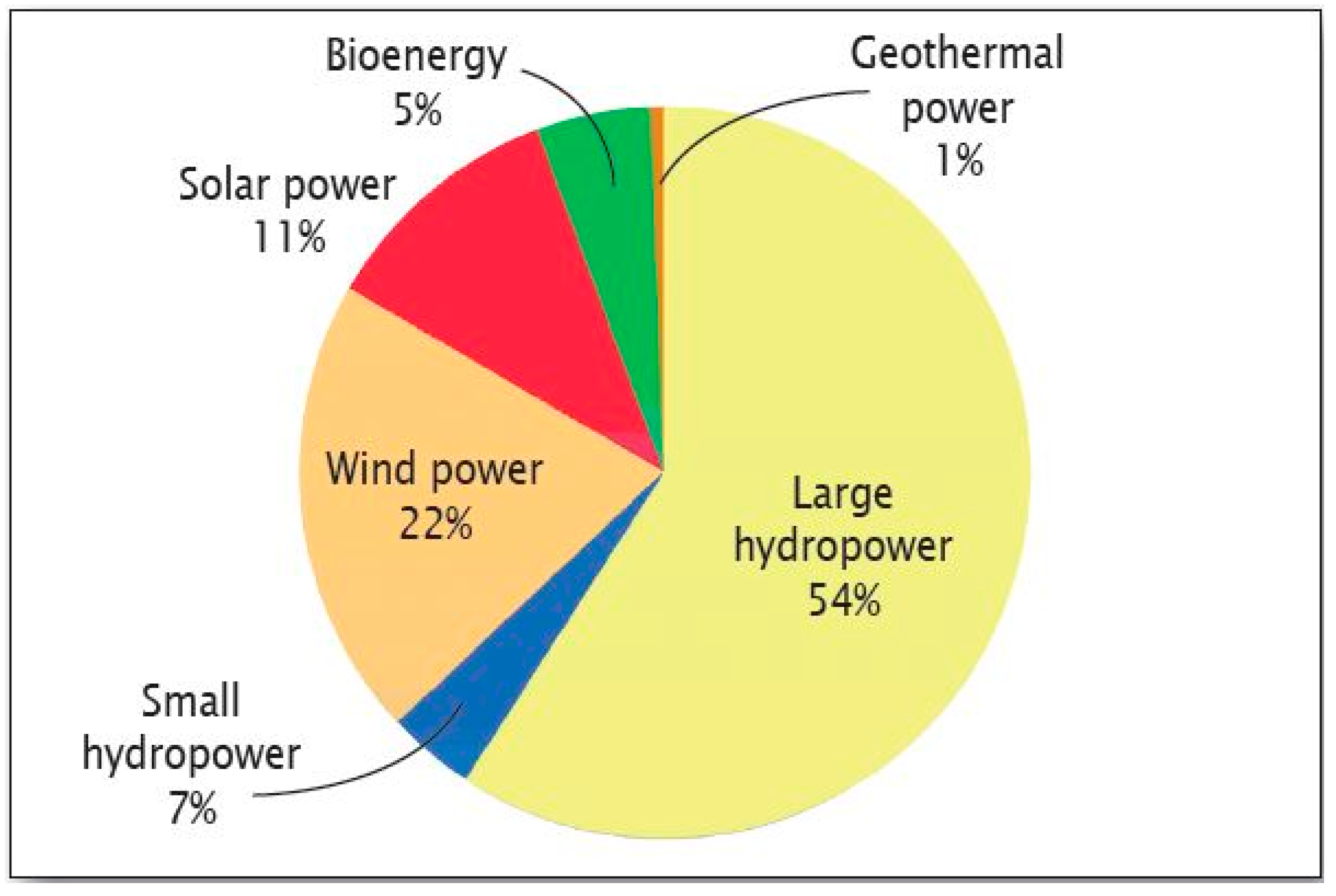
As of 2015, hydropower sources constitute around 61% of the total global renewable energy share. Of these, micro- and small-hydropower constitute around 4.5% and 7% (Figure 2), respectively. Hydropower facilities with an installed capacity between 100 kW and 10 MW are categorized under small-hydropower, while those below 100 kW are categorized under micro-hydropower [2,3]. Hydropower is one of the least expensive forms of renewable energy [2]. Moreover, despite its long history in global civilization and the increasing energy demand, more than half of the global hydropower potential still remains unexploited [4,5].

In the existing global hydro potential, small- and micro-hydropower constitute significant portions, and they play a significant role in exploiting the remaining potential, particularly in remote areas in developing and less developed countries. These hydropower sources play an important role in off-grid rural-area electrification with insignificant impact on the surrounding ecosystem [7]. Moreover, of all off-grid technologies, they constitute the least expensive form of electricity generation [6,8].

In order to best exploit the existing small- and micro-hydro potential, with the ultimate goal of meeting the growing energy demand, deploying efficient equipment to the hydropower facilities is required. The hydro-turbine is one of the most critical parts in hydropower facilities, and among other turbine designs, the cross-flow turbine is one of the most widely-applied designs in small- and micro-hydropower facilities around the globe, particularly for off-grid run-of-the-river applications.

The cross-flow hydro-turbine is relatively simple, flexible and less expensive, compared to the conventional hydro-turbines. Contrary to the developments in various computer and experiment-based optimization approaches within the last few decades, the power generation efficiency of cross-flow turbines is not yet well optimized, and insignificant research attention is given to this area. Obviously, the design methodology used to develop the turbine has a significant impact on the performance. Such a design methodology should account for not only the efficient conversion of fluid flow to mechanical energy, but also define, among others, the exact geometry of the blades, the rotational speed of the turbine and the upstream velocity that should be sustained under severe cyclic loading [9]. In this regard, some simulation-based design optimization approaches are proposed in the literature. Signagra et al. [10] investigated the reasons for the reduction of turbine efficiency and proposed a design methodology based on Computational Fluid Dynamics (CFD) simulation. The study reported by Soenoko [11] reviewed cross-flow turbine developments and suggested, among others, optimization of the nozzle construction to improve the performance of the turbine. Sammartano et al. [12] carried out computer-based tests utilizing numerical CFD and hydrodynamic analysis to obtain an optimum design aimed to come up with a theoretical framework for the turbine sequential design. However, the study was limited only to turbine configurations without a guide valve and mainly on parameters embedded in the rotor design. Anagnostopoulos and Papantonis [13], on the other hand, conducted size optimization of small hydropower plants using a then newly-developed evaluation algorithm. However, their focus was on the overall plant performance using basic plant size parameters to optimize project cost. Apart from that, there is considerable inconsistency, as regards the optimum efficiency of cross-flow turbines, in the analysis study results of various reports, both theoretical and experimental [12,14,15,16,17].

This paper has followed a new approach, in which a CFD-driven metamodel-assisted and metaheuristic design optimization tools are employed to optimize the shape of the valve profile of a T15-300 micro-cross-flow turbine design. This is one of the T-series turbine designs widely applied around the globe. The profile of the valve is generated using the NURBS (Non-Uniform Rational B-Spline) function. The main objective of the research is to improve the performance of the turbine design at the optimum valve angle. Moreover, the study aims to promote the simulation-based optimization approach for further applications on similar turbines.

The paper is organized as follows. The next section discusses in detail the turbine type employed in the research. Section 3 then discusses the NURBS function utilized to represent the valve profile. The methodologies followed in the paper are discussed in Section 4, and the numerical modeling of a case study is presented in Section 5. Thereafter, correlation studies between important hydraulic parameters in the nozzle and the entire turbine model are discussed in Section 6. Section 7 presents the sensitivity analyses’ results of the optimization parameters, while the results of the research work are discussed in Section 8. Finally, conclusions drawn from the study and recommendations are presented in Section 9.

2. Cross-Flow Turbine

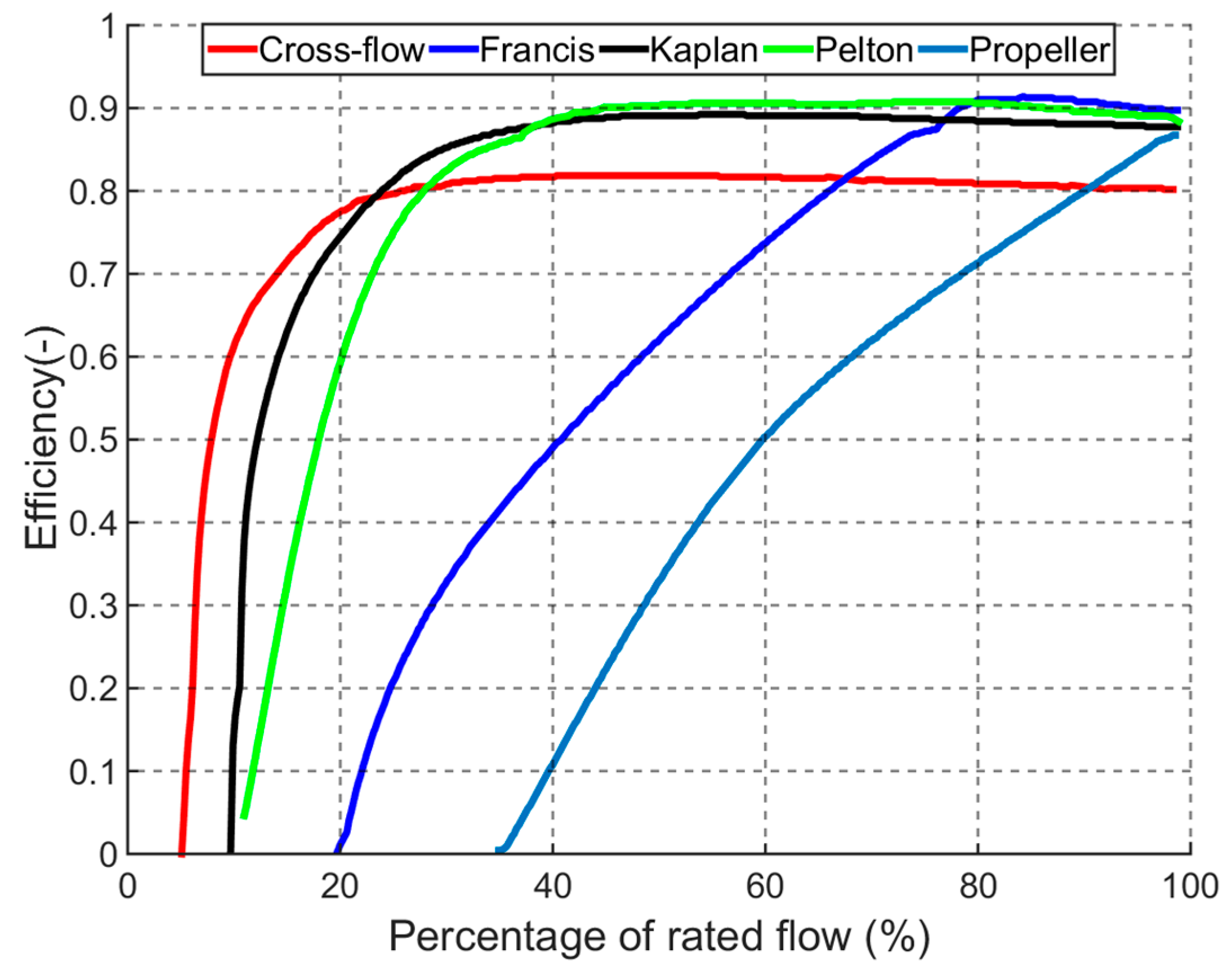
Cross-flow hydro-turbines, also known as Michell-Banki’s turbines, have been in development for decades since they were first patented by Donat-Banki in Budapest in the 1920s [16]. The benefits of the turbine, in addition to those mentioned in Section 1, are that most of cross-flow turbine parts can be manufactured with hands-on technologies [13]. Moreover, they have better power generation capability at part load conditions and favorable run-of-the-river application. Figure 3 shows the efficiency curves of various turbine designs per percentage rated flow. Despite the benefits, the figure shows that, the optimum efficiency of cross-flow turbines is lower compared to the other turbines.

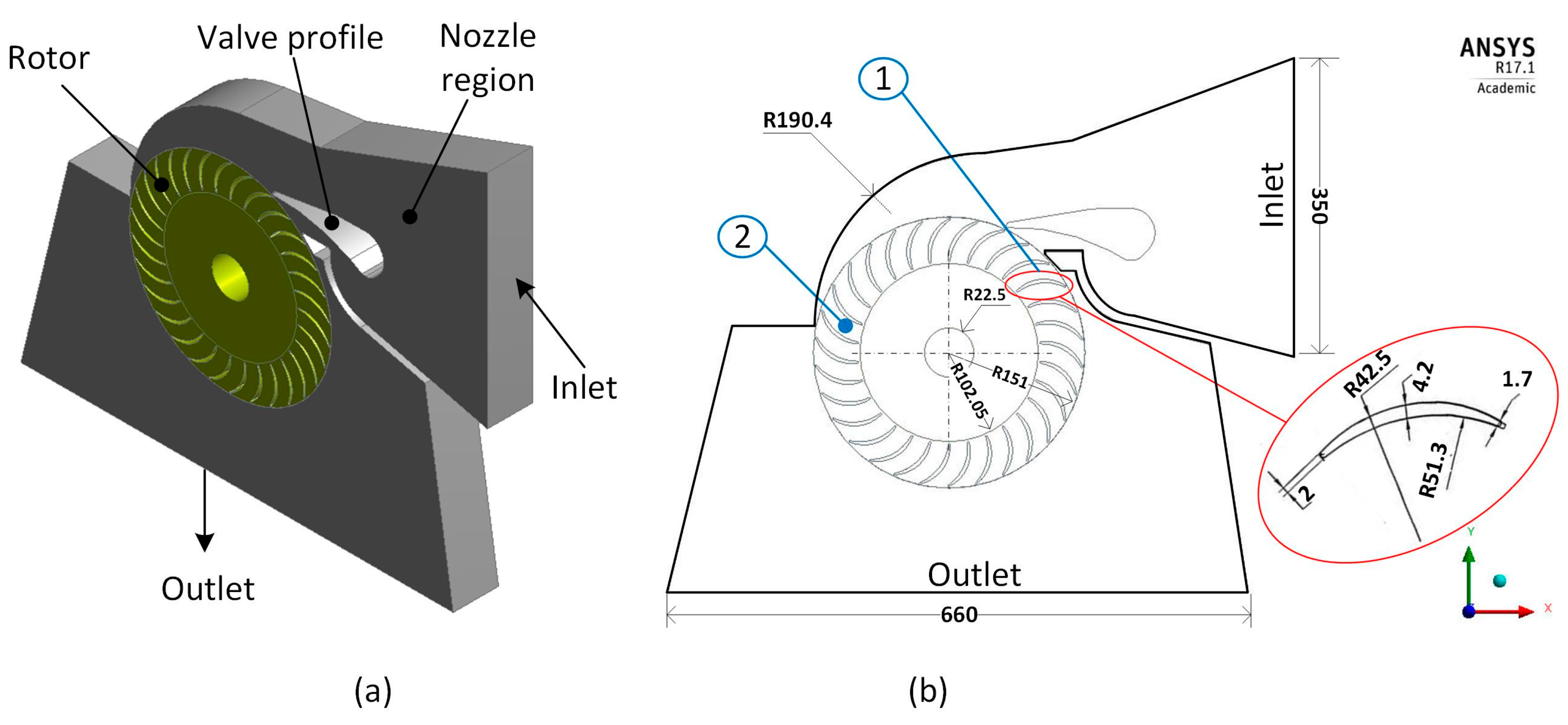
In recent cross-flow turbine design developments, nozzles, along with guide vanes or valves, are being utilized in order to control the flow and improve the turbine’s power-generating capacity [19,20]. Since the turbine is categorized as an impulse turbine, the valve is the critical part. Along with other design parameters [12], the valve design determines the magnitude of some of the important hydraulic parameters that in turn determine the power-generating capacity of the turbine. Among others, the T-series cross-flow turbine designs are the most widely-applied turbine designs that contain guide valves in their nozzles (see Figure 4). The T15-300 is one of the latest T-series models designed and has been supplied by a well-known Switzerland/Indonesia-based company called ENTEC ag, St. 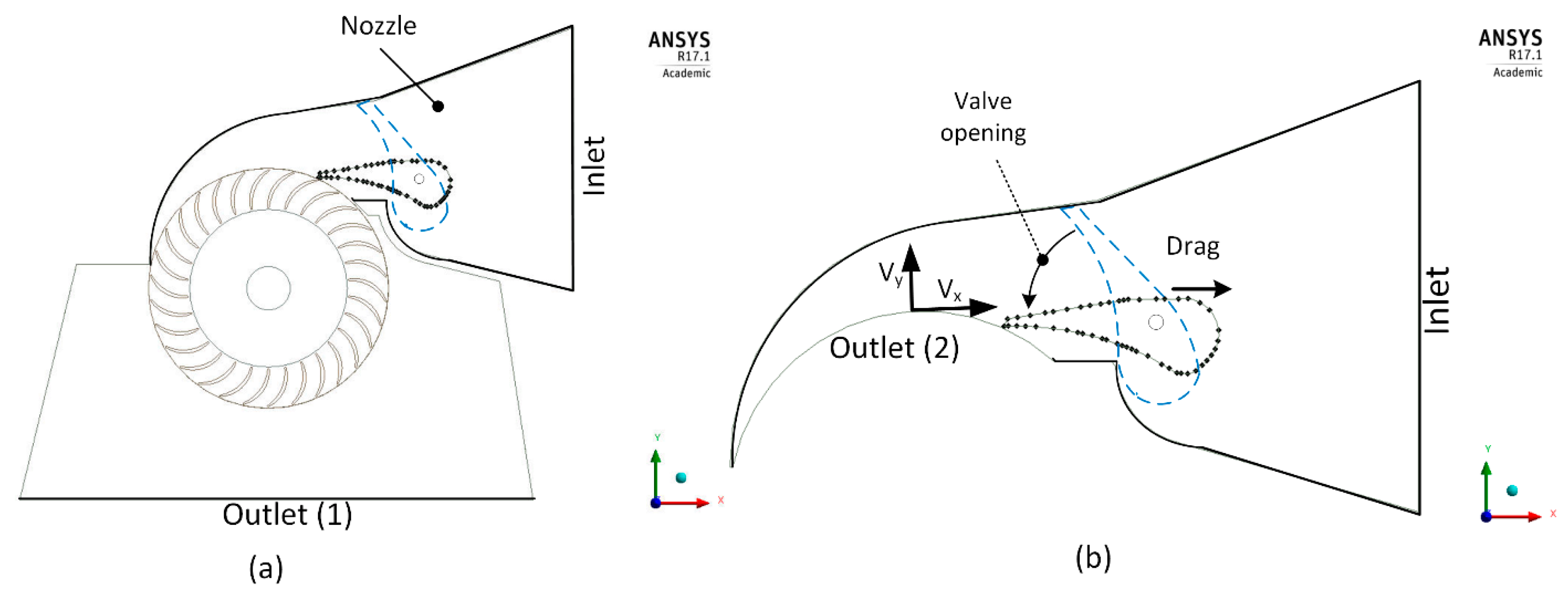(Gallen, Switzerland) [21]. For this study, we used the single-compartment design of the T15-300 turbine model, which has a width of 68 mm. As can be understood from Figure 4a, the fluid flow starts from the inlet, passes through the nozzle and then crosses the rotor before leaving through the outlet.

According to experimental investigations and numerical analysis results reported by Costa Pereira et al. [17], cross-flow turbines with a guide valve inside the nozzle have better performance as compared to those without a guide valve. 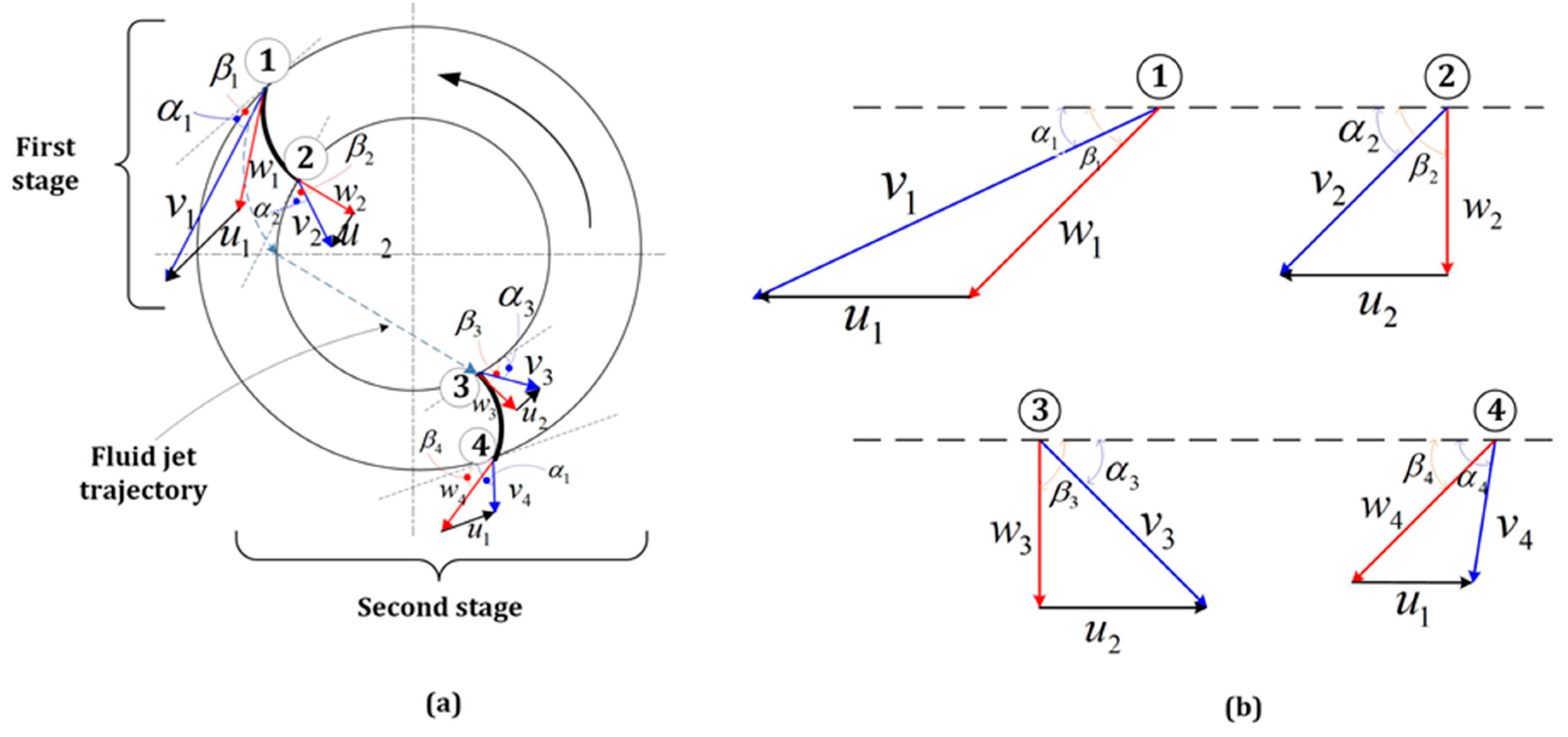Various numerical studies also concluded that the nozzle region and guide valves highly impact the fluid characteristics inside the turbine, which thus determines the performance of the turbine [11,22,23]. Fluid jet velocity components (Figure 5) at different locations of the cross-flow turbine rotor are some of the important parameters in the power conversion of the impulse type cross-flow turbines. In impulse turbines, the theoretical power conversion computation is calculated using Euler’s turbomachinery equation. The angles α₁–α₄ and β₁–β₄ (Figure 5), the angles that the actual velocity and relative velocities make with the horizontal, respectively, play important roles in transferring hydraulic and mechanical powers. The guide valve shape and rotor blades’ profile determine the magnitudes of the transferred power.

3. NURBS Function

Most Computer-Aided Design (CAD) tools utilize basis functions that are based on B-spline functions. Among others, the NURBS function is one of the state-of-the-art design basis functions applied in the latest CAD tools. NURBS can be used to describe arbitrarily-shaped curves, surfaces or bodies, have a high level of continuity and allow refinement ability on the CAD geometries [24].

The basis function is based on a parameterized recursive function, which begins from a piecewise constant value at a polynomial degree of $p=0$. For a single dimensional problem, for example, the function is formulated as:

$$N_{i,0}\left(\xi \right)=\{\begin{array}{c}1 {\xi }_i\le \xi <{\xi }_{i+1}\\ 0 otherwise \end{array}$$

(1)

For polynomial functions of a higher degrees, $p\ge 1$, the function can be recursively obtained using Equation (2),

$$N_{i,p}\left(\xi \right)=\frac{\xi -{\xi }_i}{{\xi }_{i+p}-{\xi }_i}{N}_{i,p-1}\left(\xi \right)+\frac{{\xi }_{i+p+1}-\xi }{{\xi }_{i+p+1}-{\xi }_{i+1}}{N}_{i+1,p-1}\left(\xi \right)$$

(2)

where: $N_{i,p}$ is the basis function of the polynomial degree $p$ with knot index $i=1,2,\dots ,n$. $\xi$ determines knot values from a given knot vector $\Xi =\left\{{\xi }_1,{\xi }_2, {\xi }_3,\dots ,{\xi }_{n+p+1}\right\}$. The B-Spline basis curve function, $C_b\left(\xi \right)$, is given by Equation (3).

$$C_b\left(\xi \right)={\displaystyle \sum }_{i=1}^n{N}_{i,p}\left(\xi \right)B_i$$

(3)

where $B_i=\left\{b_1,b_2,b_3,\dots ,b_n\right\}$ are the corresponding control points.

NURBS differs from B-spline in such a way that it introduces a weighting value for the corresponding control points to enable local control of the design variables. The NURBS curve equation is given as,

$$C_n\left(\xi \right)={\displaystyle \sum }_{i=1}^n\frac{N_{i,p}\left(\xi \right)w_i}{({\sum }_{i=1}^n{N}_{i,p}\left(\xi \right)w_i)}{B}_i={\displaystyle \sum }_{i=1}^n{R}_{i,p}{B}_i$$

(4)

$$R_{i,p}=\frac{N_{i,p}\left(\xi \right)w_i}{({\sum }_{i=1}^n{N}_{i,p}\left(\xi \right)w_i)}$$

(5)

where $R_{i,p}$ is the NURBS basis function and $w_i$ are the given weighted values for the control points.

4. Methodology and Approaches

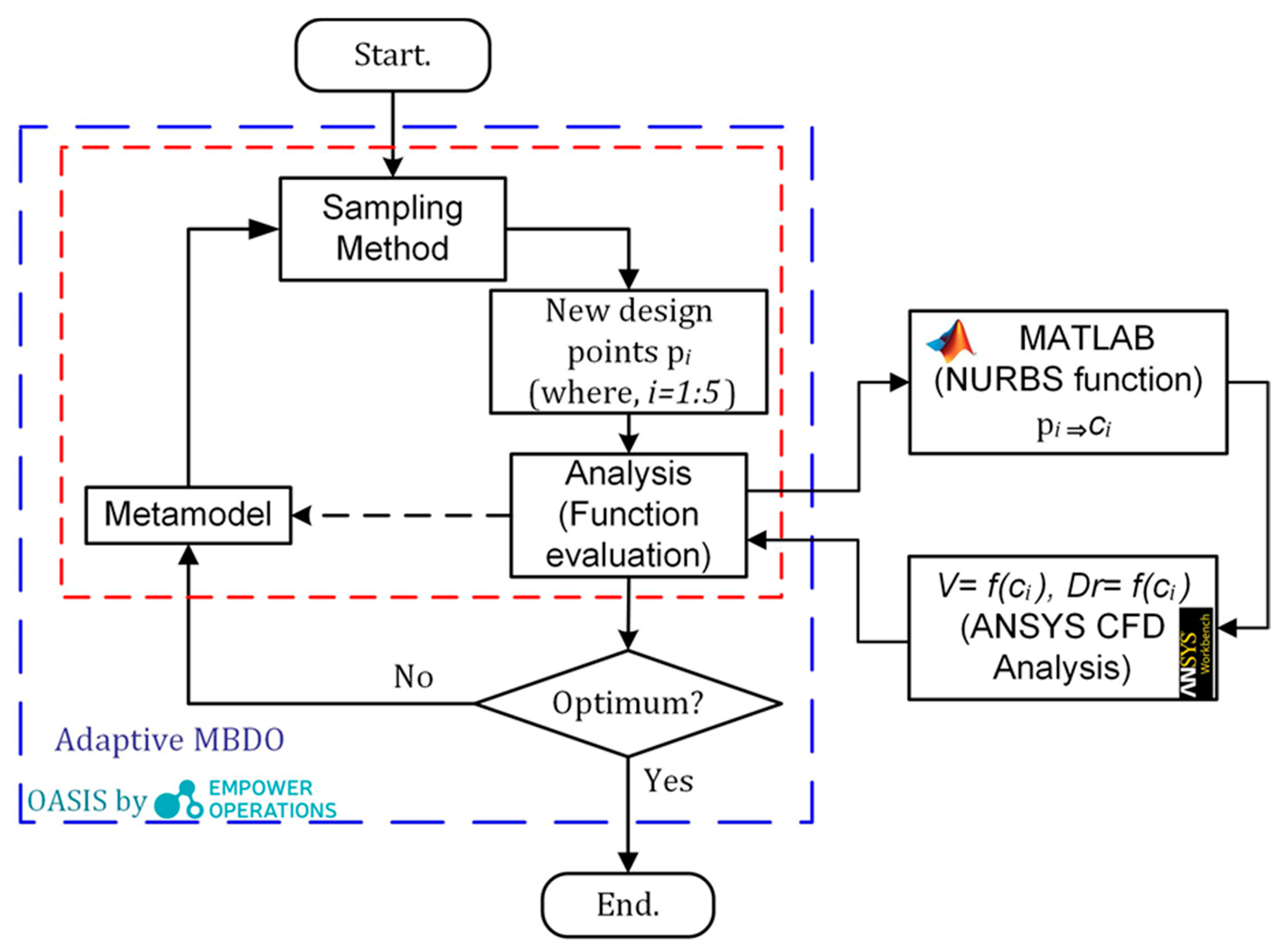
In this study, a new optimization approach has been employed to optimize the design of the valve profile in the nozzle of the cross-flow turbine under consideration. The optimization approach, illustrated in Figure 6, interconnects an optimization tool, a curve function and a modeling and analysis tool. In this approach, two optimization methods have been utilized. The first method, a Multi-Objective Metamodel-Assisted Optimization Method (MO-MMAO), uses the Optimization Assisted System Integrated Software (OASIS) optimization tool. The optimization tool, OASIS [25], has been developed for the optimization of computationally-expensive implicit problems. It was originated from the Product Design and Optimization Laboratory (PDOL) at Simon Fraser University, Canada, and developed and marketed by Empower Operation Corp (V1.3, Surrey, BC, Canada). OASIS incorporates various optimization algorithms, which are assisted by various metamodels, machine learning, statistical analysis and other tools. The optimization tool follows a direct sampling strategy, where the metamodel adaptively updates itself during the optimization process [26]. For this study, the Multi-Objective Global Optimization (MOGO) algorithm of the tool has been used. The second optimization tool is the well-known metaheuristic optimization tool, Genetic Algorithm (GA). It is a population-based optimization tool motivated by the evolutionary concept of survival of the fittest [27].

In the general approach, which employs either of the two optimization tools, a MATLAB (MathWorks, Inc., Natick, MA, USA) script is used to generate construction points from a NURBS function with the construction points being used to generate the profile of the valves of the cross-flow turbine in the modeling and analysis tool, i.e., ANSYS Workbench (ANSYS, Inc., V17.1, Canonsburg, PA, USA) [28].

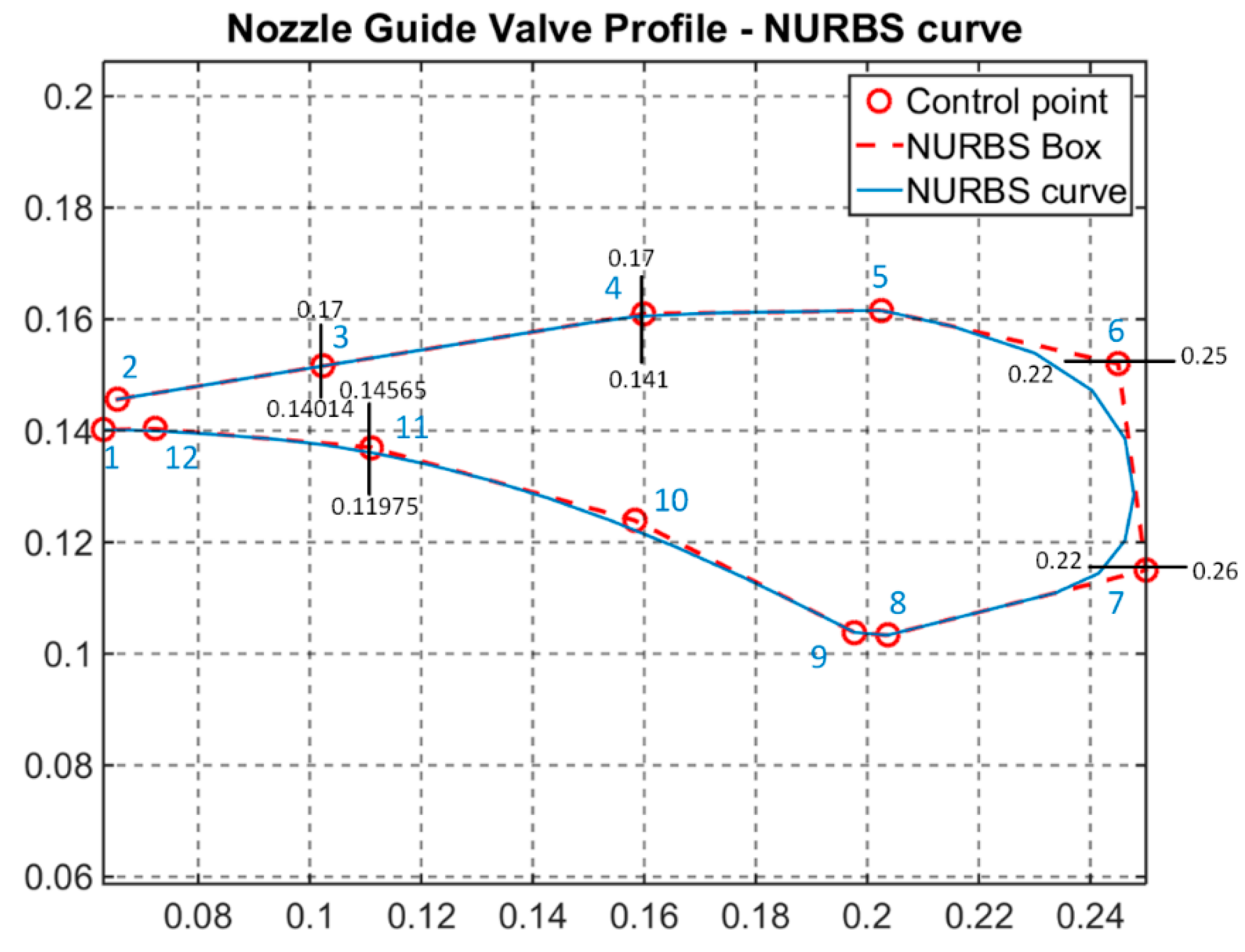
The MATLAB script uses a total of twelve (12) control points (see Figure 7) to generate a second-order polynomial NURBS curve equation [29]. Of the 12 control points, x or y-coordinates of only five selected control points are selected as optimization parameters: the y-coordinates of Control Points 3, 4 and 11 and the x-coordinates of Control Points 6 and 7 are the parameters chosen. These parameters are represented by P_i (where i = 1–5). The remaining control points maintain their original design values as they are assumed to be less important in the optimization, but critical for the overall valve operation. For instance, Control Points 1, 2, 8 and 9 are at critical locations of the valve and are used for proper sealing when the valve is in a closing position (Figure 8a), while Point 5 maintains the gap between the valve profile and the shaft outer diameter, which is used to maneuver the valve. A total of fifty (50) construction points is generated from the NURBS curve equation. The x- and y-axis components of the 50 construction points are mapped to 100 design parameters in the ANSYS Workbench CAD modeling tool. The construction point parameters are represented by C_i (where i = 1–100). Based on the sensitivity to the objectives (see Section 7), the five optimization parameters are given different weighting values in the NURBS function.

The other important concept in the optimization approach is to separately optimize the nozzle region (Figure 8b). We have followed this concept for three important reasons:

(i).

Since the turbine is assumed as the impulse turbine, this part of the turbine plays a critical role in the entire power generation;

(ii).

It enables us to easily identify and control the important hydraulic parameters at the nozzle that are important in the entire power transfer and are mainly affected by the shape of the guide valve;

(iii).

It reduces the computational cost in the optimization process.

It is important to note that the change in the trends of the output parameters from the separate nozzle design are initially correlated with the change in the trends of the important output parameters of the full turbine design due to the change of valve angle (with respect to the turbine’s performance), which is discussed in Section 6. After the optimization process, a comparison of the optimized valve designs with the original design is carried out using the full turbine model.

The multi-objective optimization problem has two objectives and two constraint functions. The two objectives of the optimization, based on the correlation studies are (1) minimizing the x-component (maximizing the magnitude) of the area-weighted average velocity ($V_x$) of the nozzle outlet fluid and (2) minimizing the drag force (Drag) on the valve profile. The general formulation of the problem is given in Equation (6). Both objective functions are obtained after the CFD computation of the turbulent numerical model using the implicit analysis tool, ANSYS Fluent tool:

$$\mathrm{Minimize}{V}_x=f\left(P_i\right) \mathrm{and}Dr=f\left(P_i\right);\left(i=1, 2, \dots 5\right)$$

$$\mathrm{Constraints} C\left(P_i\right)\le 0, (P_1-P_2 \le 0,\mathrm{and}{P}_5-P_1 \le 0)$$

(6)

$$P_i \in \left[P_{iL}, P_{iU}\right]$$

where $V_x$ and $Dr$ represent the x-component of the area-weighted average velocity at the nozzle outlet and drag force functions; where both are functions of the optimization parameters ($P_i$); $C\left(P_i\right)$ represents the constraint functions respectively; and $P_{iL }\mathrm{and} P_{iU}$ are the lower and upper bounds of the optimization parameters, respectively.

The lower and upper bounds of the parameters are obtained from the design configuration of the original turbine design so that they should not create any irregular valve profile and unacceptable nozzle region; see

Table 1. Design points, lower and upper bound values of the optimization parameters.

Name of Points	${\mathit{P}}_1$ (m)	${\mathit{P}}_2$ (m)	${\mathit{P}}_3$ (m)	${\mathit{P}}_4$ (m)	${\mathit{P}}_5$ (m)
Design point	0.15160	0.16092	0.24500	0.25000	0.13700
Lower bound	0.14014	0.14100	0.22000	0.22000	0.11972
Upper bound	0.17000	0.17000	0.25000	0.26000	0.14565

. Therefore, the parameters are bounded inside the nozzle region. The same principle is followed when the constraints on the design variables are determined from the turbine configuration.

5. Numerical Modeling

Based on our experience of comparative studies of the applications of different numerical models on similar problems and various other numerical studies, the standard K-ε numerical model [30,31] is found to best represent the fluid flow inside the cross-flow turbine. According to studies and user guides of simulation tools, this model is robust, economical and provides reasonable accuracy not only for the current problem, but also for a wide range of problems. Therefore, in this paper, we have employed the standard K-ε model for both the time-dependent (transient) and steady state analyses in both the separate nozzle and entire turbine models. In the general transport equation for the standard K-ε model, the turbulence kinetic energy and the rate of dissipation, k and ε, respectively, are obtained from Equations (7) and (8) [30]. A scalable wall function is selected for the near-wall treatment.

$$\frac{\partial }{\partial t}\left(\rho k\right)+\frac{\partial }{\partial x_i}\left(\rho k{V}_i\right)=\frac{\partial }{\partial x_j}\left[\left(\mu +\frac{{\mu }_t}{{\sigma }_k}\right)\frac{\partial k}{\partial x_j}\right]+G_k+G_b-\rho \epsilon -Y_M+S_k$$

(7)

$$\frac{\partial }{\partial t}\left(\rho \epsilon \right)+\frac{\partial }{\partial x_i}\left(\rho \epsilon V_i\right)=\frac{\partial }{\partial x_j}\left[\left(\mu +\frac{{\mu }_t}{{\sigma }_{\epsilon }}\right)\frac{\partial \epsilon }{\partial x_j}\right]+C_{1\epsilon }\frac{\epsilon }{k}\left(G_k+C_{3\epsilon }{G}_b\right)-C_{2\epsilon }\rho \frac{{\epsilon }^2}{k}+S_{\epsilon }$$

(8)

where $\rho$, $\mu$ and $V_i$ are density, viscosity and velocity vectors of the flowing fluid, respectively. ${\sigma }_k$ and ${\sigma }_{\epsilon }$ are the turbulent Prandtl numbers for k and ε, respectively; whose default values in the tool are used for our analyses. $G_k$ and $G_b$ are the generation turbulence kinetic energy due to the mean velocity gradients and buoyancy, respectively; however, the generation buoyancy is negligible for this problem. $Y_M$ represents the contribution of the fluctuating dilation in compressible turbulence, which is negligible in our analyses. $S_k$ and $S_{\epsilon }$ are the source terms for kinetic energy and dissipation, which are not applicable for this problem. $C_{1\epsilon }$, $C_{2\epsilon }$ and $C_{3\epsilon }$ are given constant values; $\frac{\partial }{\partial t}$ is the gradient vector with respect to time; $\frac{\partial }{\partial x_i}$ and $\frac{\partial }{\partial x_j}$ are the spatial gradient vectors at the $i$ and $j$ coordinates.

The turbulent viscosity term, ${\mu }_t$, is computed using Equation (9), where the term $C_{\mu }$ is a constant value. All constants are listed in

Table 2. Given and standard values for constant variables.

Numerical Model Constants	Values
$\rho$ (kg/m3)	998.2
$\mu$ (kg/ms)	0.001003
$C_{\mu }$ (-)	0.09
${\sigma }_k$ (-)	1
${\sigma }_{\epsilon }$ (-)	1.3
$C_{1\epsilon }$ (-)	1.44
$C_{2\epsilon }$ (-)	1.92

with their corresponding valves.

$${\mu }_t=\rho C_{\mu }\frac{k^2}{\epsilon }$$

(9)

In order to identify an allowable and efficient head for the analyses, an efficiency curve study from steady numerical analyses on the full turbine models is carried out at various flow rate ratios computed from the head ranges from 5–22.2 m. The mass flow rate at each head over the mass flow rate at the maximum head is calculated to find each flow rate ratio. Based on the result, the average allowable head of 12.5 m was maintained for all analyses, as it is where the model provides the maximum computed hydraulic efficiency. In addition, the valve angle position is set at its maximum opening position where the maximum numerical power output is obtained. Moreover, for all simulations on the full turbine model, the rotor speed is maintained at 360 rpm.

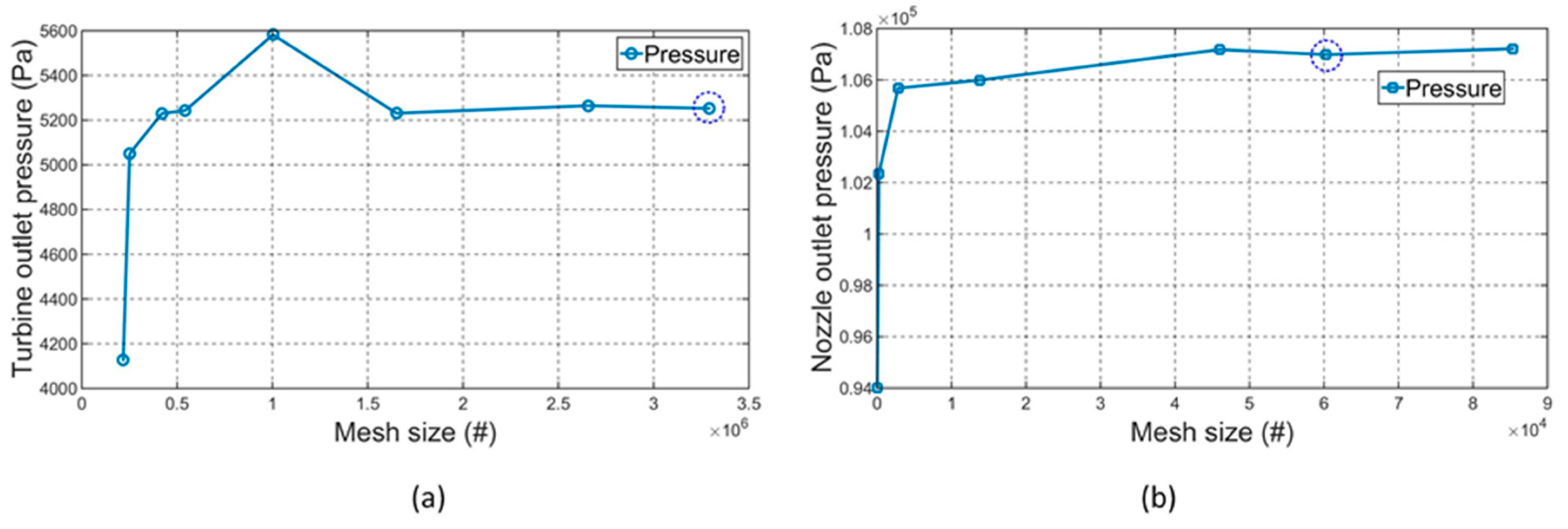
5.1. Meshing Qualities and Convergence

After a number of trials and convergence tests, valid mesh sizes of the full turbine model and the separate nozzle model are chosen; see Figure 9. The meshing details and characteristics of the selected meshes of the models (circled in blue in the figures) are shown in

Table 3. Meshing size details of the full turbine geometry and separate nozzle geometry.

Geometries	Housing Elem. Size	Rotor Elem. Size	Total Elem. Size	Mesh Min. Size	Mesh Max. Face Size	Max. Tet Size
Full turbine geometry	57,662	3,234,243	3,291,905	0.0005	0.0065	0.015
Separate nozzle geometry	60,270	-	60,270	0.00035	0.0045	0.015

Elem. stands for mesh element and Tet stands for tetrahedral.

. The total area-weighted average pressure values at the outlets of the models were the convergence test parameters in the test; whereas, built-in mesh quality measures in the meshing tool of ANSYS Fluent, such as element quality, skewness and orthogonal qualities of the meshes, are checked while maintaining the meshing quality. Moreover, due to the configuration of the problem and the existence of interfacing bodies, the unstructured meshing method is selected, and local meshing techniques are used to refine meshes around the small-sized rotor blades’ edges and surfaces. The mesh qualities are then controlled to fall within the recommended range of values of the mesh quality measures.

5.2. Solution Methods

To solve the transport equations for the standard K-ε numerical model in CFD tool, the SIMPLE algorithm scheme has been employed to compute the pressure-velocity coupling, and least squares cell-based method has been used to compute the gradient in the spatial discretization. Considering the complex geometry of the rotor and the interface between the housing and rotor domains, the second order method has been employed to compute the pressure and the second order upwind to compute the momentum, turbulent kinetic energy and turbulence dissipation rate equations in the spatial discretization. In both the full turbine and separate nozzle models, all walls are given a no-slip condition, and the outlet surfaces are given pressure-outlets with zero gauge pressure boundary conditions.

After solving the transport equations, the area-weighted average values, which are the valid velocity magnitudes of the numerical fluid flow, are considered to compute the actual velocities at the outlet surfaces of both geometries. In addition, the x-components of the combined pressure and viscous forces are used to determine the drag force on the guide valve surface. Pressure and viscous forces ($\overline{F_p}$ and $\overline{F_v}$, respectively) are computed based on their computed and user-determined reference values; for instance, the pressure force is computed as Equation (10). On the other hand, the total moment load vector, moment coefficients, output hydraulic power and numerical efficiencies are computed using Equations (11)–(14), respectively.

$$\overline{F_p}={\displaystyle \sum }_{i=1}^n\left(P-P_{ref}\right)A\widehat{n}$$

(10)

$$\overrightarrow{M}=\overrightarrow{r}\times \overrightarrow{F_p}+\overrightarrow{r}\times \overrightarrow{F_v}$$

(11)

$$C_m=\frac{M}{\frac{1}{2}{\rho }_r{V}_r^2{A}_r{L}_r}$$

(12)

$$P_o=M.\omega$$

(13)

$$\eta =\frac{M.\omega }{Q_{in}\left(P_{in}-P_{out}\right)/\rho }$$

(14)

where $P$ and $P_{ref}$ are the computed and user-determined reference pressures (Pa), respectively; $\overrightarrow{r}$ and $\overrightarrow{M}$ are the moment arm and moment vectors. $C_m$ is the unit-less moment coefficient. ${\rho }_r$, $V_r$, $A_r$ and $L_r$ are the reference density (in kg/m³), velocity (m/s), area (m²) and length (m) values, respectively, set in the analysis tool. $M$, $Q_{in}$ and $\omega$ are the magnitude values of moment (Joules), mass flow rate (kg/s) and rotational speed of the rotor (rad/s), respectively.

6. Correlation Study between the Separate Nozzle and Full Turbine Models

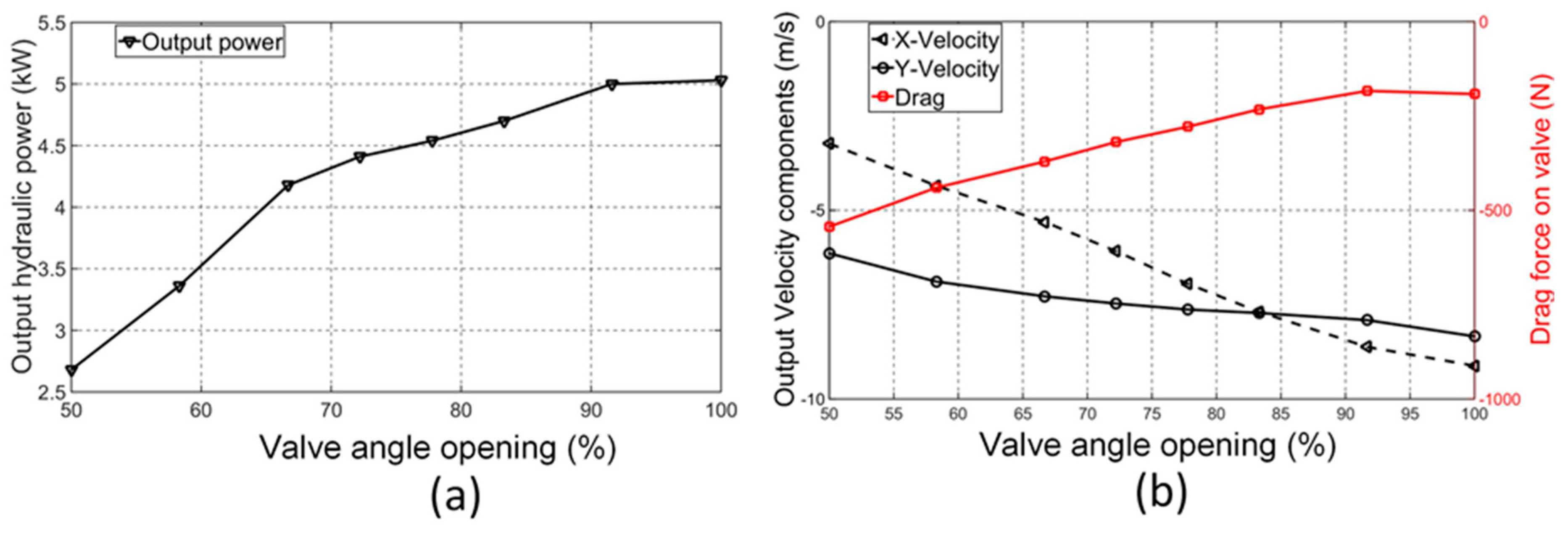
To identify important output parameters from the separate nozzles that have a direct impact on the performance of the turbine and to understand their trend with the change of the valve design, a correlation study between the separate nozzle and full model was carried out. While conducting this study, several numerical simulations were run on both the separate nozzle and full turbine models at different valve positions, and their results have been analyzed. The valve angle opening position was set to range from 50–100% opening. The other boundary conditions, such as inlet head, rotational speed of the rotor for the full model, numerical model settings and the geometric parameters except valve position, are set constant in all analyses. The output power is computed from the full turbine model, and various output parameters are studied from the nozzle model. The main purpose of this correlation study is to identify the two output parameters from the nozzle model with higher impact on turbine performance and set them as objective parameters.

As depicted in Figure 10a, the results show that the output power increases as expected with the valve opening from 50–100% from the closing position. The simulation results from the separate nozzle model, Figure 10b, reveal that the drag force on the valve profile and the x-component of the area-weighted average velocity (X-Velocity) from the nozzle outlet surface have a visible correlation with the output power. The velocity magnitude has a direct relation to the output power, while the drag force has an inverse relation. Therefore, it is valid to set the objectives of the optimization to minimize the x-component of the velocity at the nozzle outlet and minimize the drag force on the valve profile.

7. Sensitivity Analyses

To assign logical weighting values to the corresponding control points for the NURBS curve, the significance of the optimization parameters for the output objective parameters should be studied. Such significancy studies (sensitivity analysis) can be achieved by employing the concept of the statistical Design Of Experiment (DOE). The factorial DOE method is a widely-applied method in the scientific community. For this study the fractional factorial design method has been applied to estimate the direct effects of the five optimization parameters ($P_i$) on the responses of the two objective parameters (V and Dr) in the separate nozzle model. Unlike the full factorial experimental design, the fractional method does not estimate all the interaction effects of the parameters, but can correctly estimate the main effects with fewer runs, compared to the intensive full factorial.

A three-level five-parameter analysis with two responses was employed. Level 1 is the lower bound; Level 2 is the design point; and Level 3 is the upper bound. The custom optimal factorial design option with random sampling from the Design-Expert tool [32] dictated that 26 combinations of samples should be run. The settings of the other important parameters are carefully controlled based on the standard recommendations of the tool.

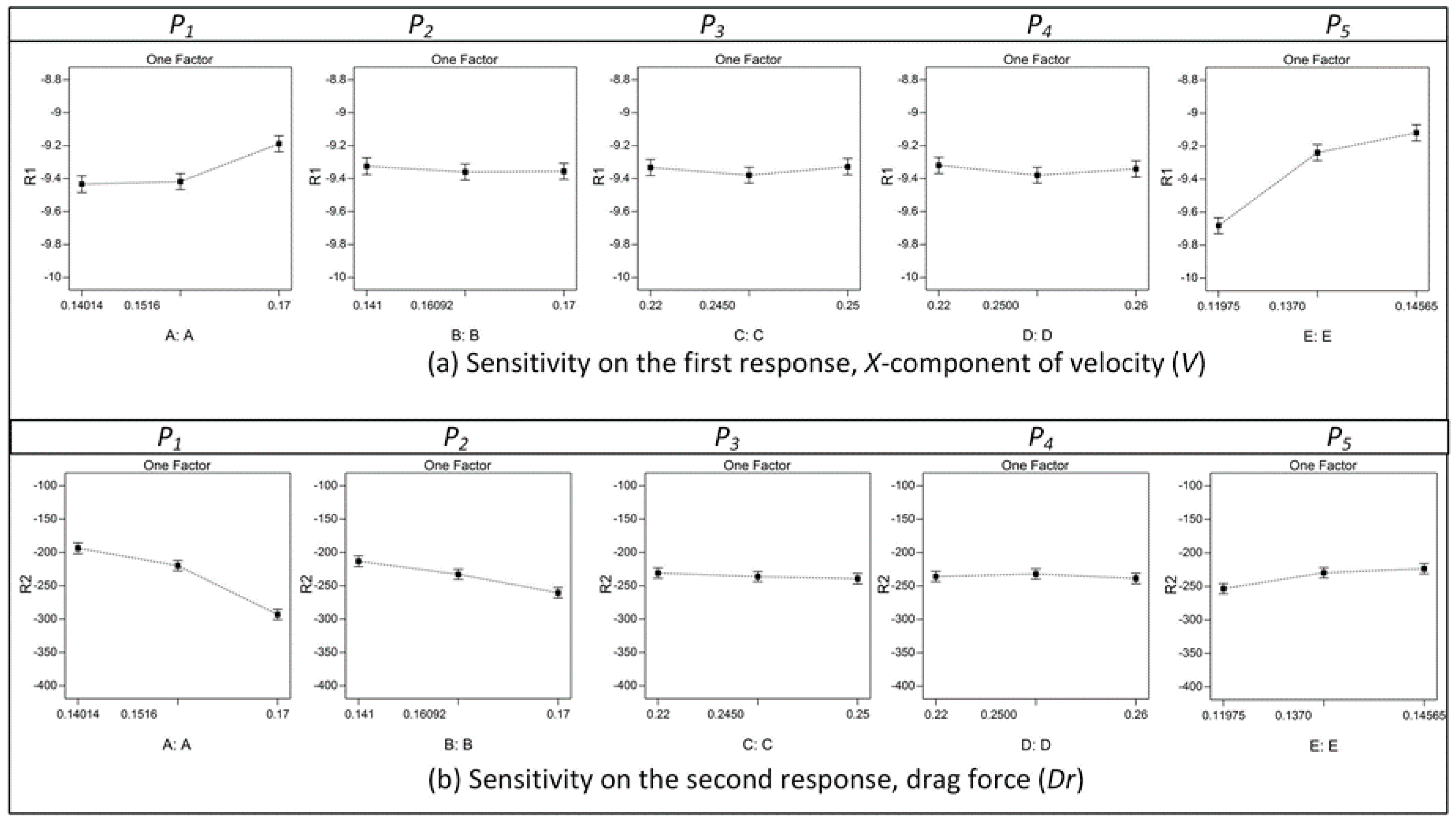
According to the sensitivity test results (Figure 11), the first and fifth parameters ($P_1$ and $P_5$) are highly sensitive to both objective parameters, compared to the other three, while the second parameter ($P_2$) is more significant to the second response than the remaining two.

Therefore, the corresponding control points for the first and fifth parameters are given higher weights in the NURBS curve function, so that more construction points will be generated from their surrounding points on the curve, thus generating smooth curves in their vicinity. Note that the total number of construction points in the NURBS curve can be determined in the function’s MATLAB script by the user depending on the interest. On the other hand, the two least sensitive parameters ($P_3$ and $P_4$) are given only fair weighting values.

8. Results and Discussion

The MMAO optimization was performed by setting the OASIS tool to a maximum function evaluation of 100 (based on authors’ previous experience on similar problems). Apart from the default convergence tolerance settings, the maximum number of evaluations is used as a stopping criterion for the optimization process in the tool. In the multi-objective GA optimization, the number of generations is set to be six and the stall generation limit of five are set as stopping criteria. The population size is chosen to be 20. This combination gives at least 100 function evaluations in the GA optimization process. The same computational workstation was used for both optimization processes: HP Z600 of processor Model Intel(R) Xeon(R) X5650 (HP Inc., Palo Alto, CA, USA) with two processors each around 2.67 GHz capacity. The optimization results and the comparative analyses are discussed in detail in Section 8.1 and Section 8.2, respectively.

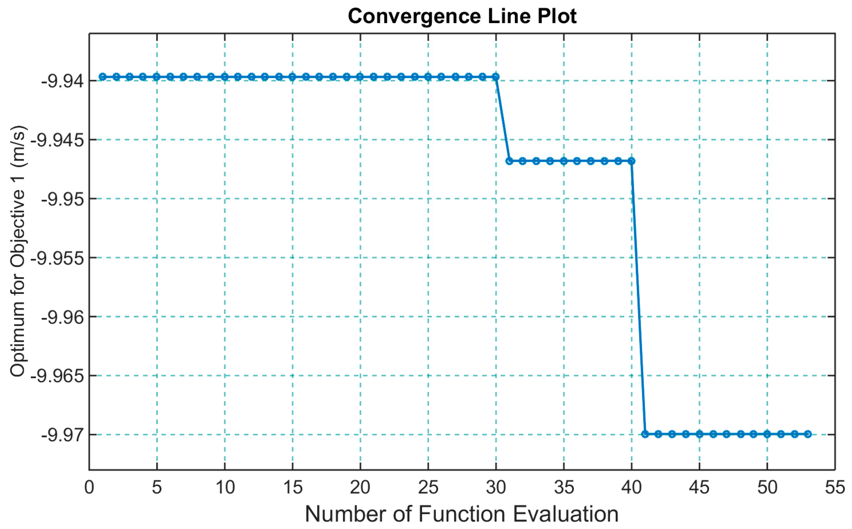
8.1. Optimization Results

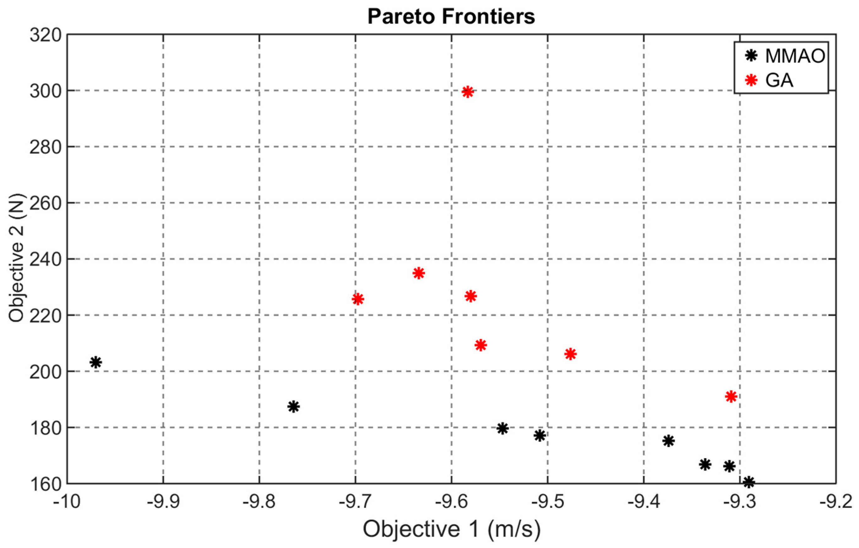
Figure 12 shows the convergence plot with the number of function evaluations for the Metamodel-Assisted Optimization (MMAO), i.e., OASIS optimization process; it can be observed that the optimization converged at the 53rd function evaluation count. The total time elapsed was 2 h, 50 min and 26 s. The best Pareto point (with respect to the turbine’s performance) from the Pareto frontier points, shown in Figure 13, is taken as the best optimum point (

Table 4. Parameter values from the optimization results and steady analyses’ results.

Turbine Model	${\mathit{P}}_1$ (m)	${\mathit{P}}_2$ (m)	${\mathit{P}}_3$ (m)	${\mathit{P}}_4$ (m)	${\mathit{P}}_5$ (m)	Power Output (Watt)
Original	0.151600	0.160920	0.24500	0.25000	0.13700	4841.83
GA	0.143077	0.16730	0.23089	0.24575	0.13308	5070.89
MMAO (OASIS)	0.142430	0.15588	0.23567	0.24059	0.12091	5099.85

) for our further comparative analyses.

Unlike the MMAO optimization, the multi-objective GA optimization carried out a total of 121 function evaluation counts, which led to the fact that it took around 3.69 h. Seven (7) Pareto front points are returned from the optimization process (Figure 13); similarly, the best Pareto point (Table 4) is taken as the best optimum point for our further comparative analyses.

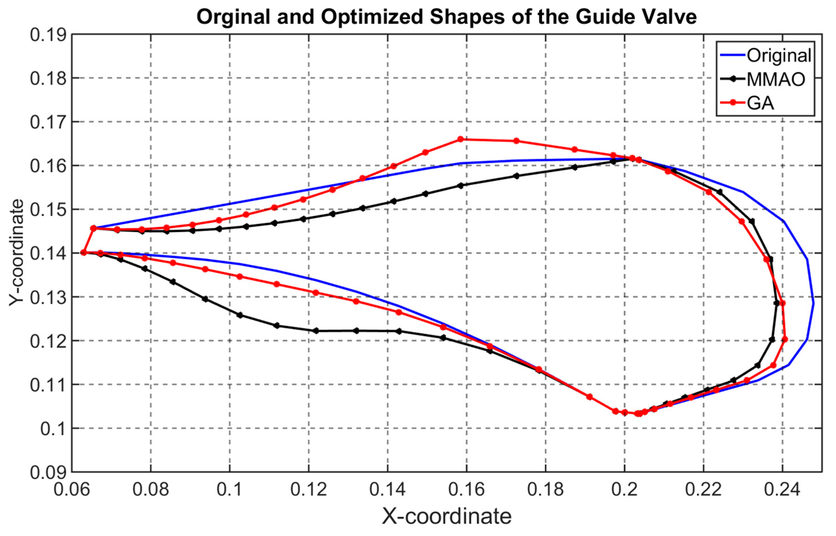
Apart from the differences in computational time and number of the function evaluations, a difference is also observed in the shape of the optimized valve models (see Figure 14). However, the shapes from both methods are not as complex as one may expect.

8.2. Comparative Analyses and Discussions

To see the actual impact of the optimized shapes on the full turbine design, both steady and transient CFD analyses (simulations) have been carried out and the responses collected and compared against the original design. In the transient simulations, the time step size was set at 0.001 and ran for 1000 time steps. Given the rotational speed of the rotor, around 5.83 rotations are expected in one second. An output parameter that has a direct relation to the performance of the turbine, which is the surface moment about the rotational axis of the rotor, has been chosen for comparison. The moment is the result of the effect of the sum of both pressure and viscous forces (Equation (11)). Time-dependent responses of the moments have been collected from the surfaces of the two parts:

(i).

From the surfaces of one of the rotors’ blade (1); see Figure 4b.

(ii).

From the surfaces of the entire set of rotor blades (2).

Note that in order to avoid some irregularities seen on the responses at the beginning of the first cycle, it was decided to consider the data from the second cycle in both cases of the comparative studies.

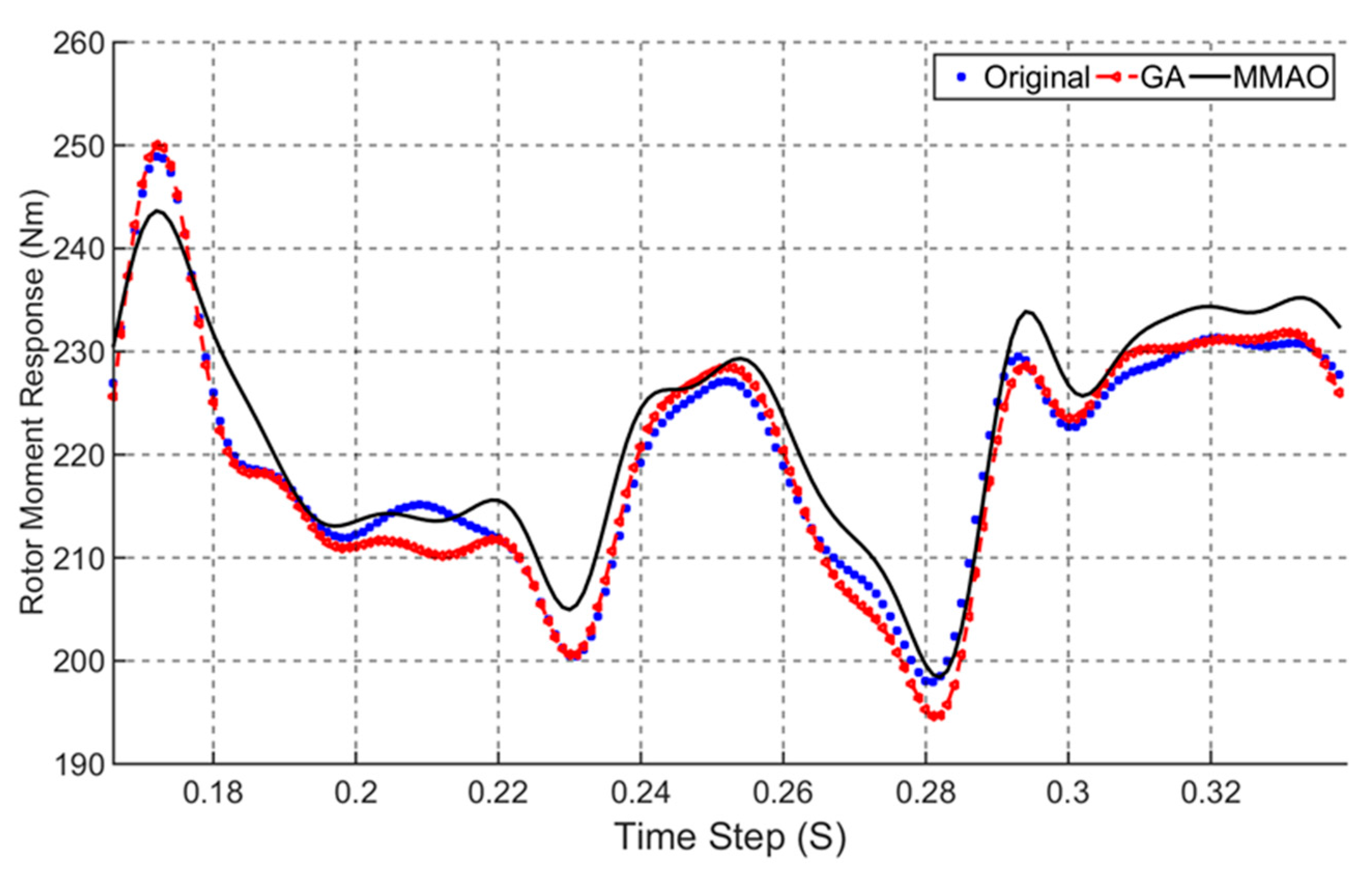
The moment responses and their peak values of the second rotation (cycle) from the transient analyses are examined using comparative graphs. The comparative graph of the moment responses from the entire set of rotor blade surfaces, depicted in Figure 15, shows that both the optimized designs return better responses than the original design at most of the time steps, except at the beginning of the cycles. On the other hand, the responses from the MMAO optimized design are seen to outperform the GA-optimized design. Therefore, as can be seen from Table 4, the total power output of the MMAO-optimized design from the time-independent (steady) analyses is higher than that of the other two designs.

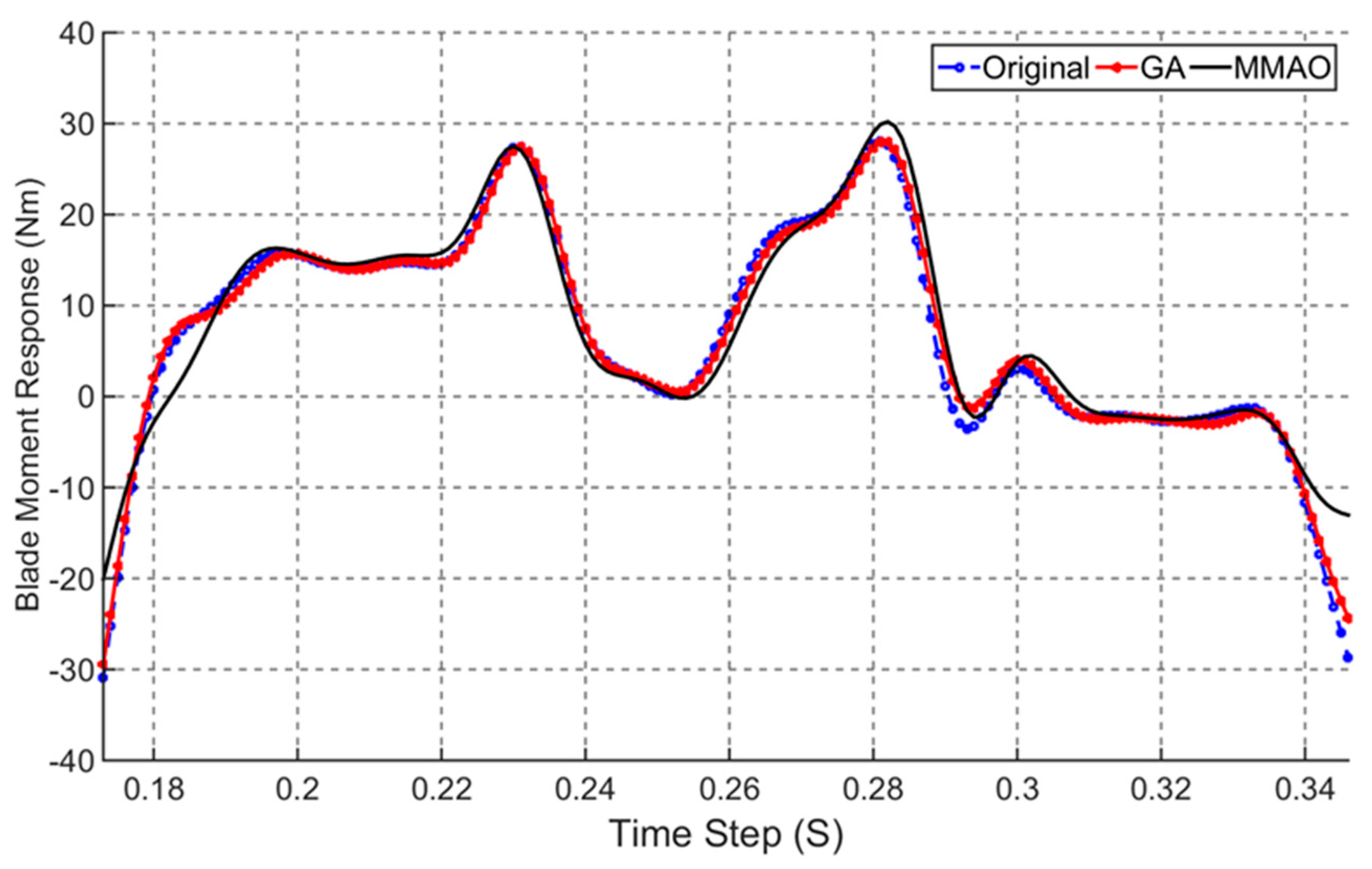
Unlike the responses from the surfaces of the entire set of rotor blade surfaces case, the plot in Figure 16 indicates that the moment responses collected from the single blade (1) show little variation. However, it is clear and possible to deduce that the optimized designs still return better responses in magnitude at most time steps than the original design.

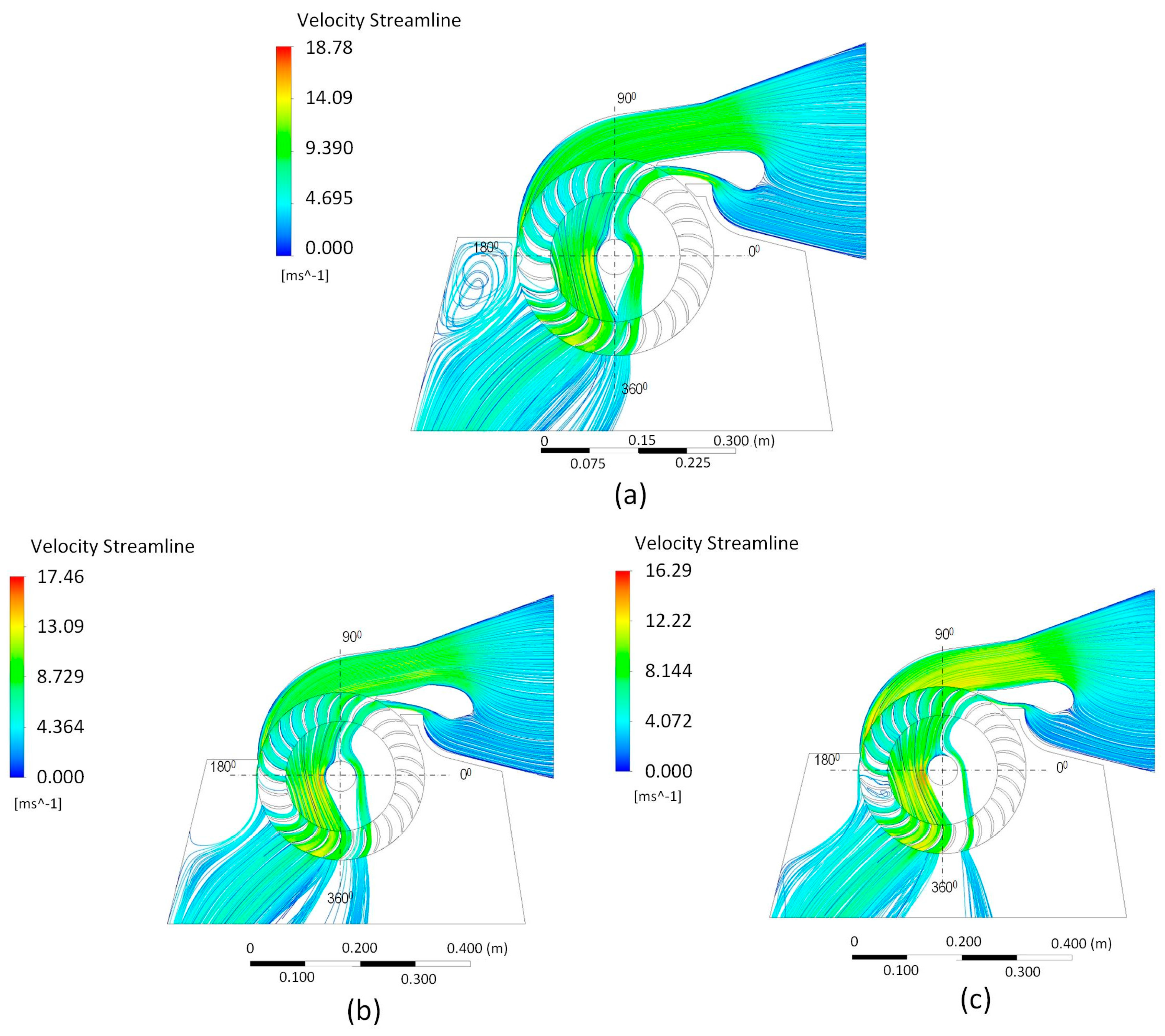
Moreover, the steady analyses’ results (Table 3) estimate a power improvement of around 5.33% and 4.73% from the MMAO-optimized design and the GA-optimized design, respectively. On the other hand, from the visual analysis of the fluid stream-band width in the first quarter of the velocity streamline from the steady analyses, Figure 17 illustrates the volumes of the ineffective fluid crossing the rotor in the three models. The optimized models have a thinner fluid stream-band width than that of the original model.

In addition, considering the ratio of the sum of all peak moment responses from the three models from the full rotor surface to the single blade surface, we have seen that an estimated average of 8.61 blades contributes to the power generation at each cycle of the rotor.

Moreover, as one can see from both moment response figures, the response curves from all models coincide in some cases, but show a similar trend in all cases, which verifies that the numerical model employed is valid and converging.

9. Conclusions and Recommendations

In this article, CFD-driven shape optimization is performed on the cross-flow turbine design. The approach provided promising results with regard to improving the performance of the cross-flow turbine. The motivation for the study is the fact that, since hydropower is one of the least expensive and most abundant renewable energy sources around the globe, efforts to improve performance by designing optimized critical parts for hydropower facilities are indispensable.

Two different optimization methods have been employed in the approach. One is the widely-applied multi-objective Genetic Algorithm (GA) optimization method, and the second is the Metamodel-Assisted Optimization (MMAO) method from the OASIS tool. Optimized models from both optimization methods showed an estimated 4.73% and 5.33% improvement on the output power, respectively, compared to the original un-optimized design model. Apart from that, the MMAO optimization process converged at fewer function evaluations and lesser processing time than its counterpart. One of the main reasons is that, unlike the GA method, the MMAO method generates samples towards the optimum region to assist the optimization process to converge with fewer function evaluations.

Therefore, we can conclude that the approach we have introduced is effective for such a shape optimization problem to improve the performance of impulse turbines. This approach can be applied to optimize the performance of similar turbines. It is also revealed through the study that the MMAO method offers a better performance design, and it is more effective than the GA method in identifying the Pareto frontier. The MMAO method has also been shown to be computationally less expensive than GA.