A Heuristic Algorithm to Compute Multimodal Criterial Function Weights for Demand Management in Residential Areas

Abstract

We present the conceptual design of a collective control scheme for appliances within a smart home. Based on the relevant energy acquisition procedures, three appliance groups are defined, modeled, and completed with an energy storage as well as a generator using renewable sources. At the following stage, a mixed quadratic optimization problem is presented, with the solution consisting in a time plan to regulate the operation of the individual devices. Importantly, the paper also proposes a heuristic algorithm securing consistent functionality of the computational process even despite the varying input and user conditions given in the receding horizon.

1. Introduction

Electricity consumption currently plays a central role in all fields of human activity. In the last 100 years, the world population has increased to such an extent that, at present, ample food or potable water to sustain the existing human community cannot be produced without electricity. In this context, however, it is also important to note that although the generation of electrical energy from fossil fuels has revolutionized the basic social processes, the resulting benefits are not without a major consequence: the irreversible changes of Earth’s environment could be largely regarded as following from the intensive use of the said fuels. The dwindling volumes and growing prices of these resources correspondingly increase the cost of energy, and the search for alternative energies has become ever more urgent. The gradual growth of energy costs is accompanied by increasing willingness on the part of users to change their behavior with the aim to cut the electricity expenditures or, in the very least, to maintain them at an acceptable level. Consumers are thus more inclined to purchase advanced energy saving devices and to install local generators of energy or technologies that facilitate its preservation and use at a later time.

This article discusses a universal method for optimal electricity consumption planning in residential areas and presents a software implementation to validate the related procedures. Based on end user demands, the technique coordinates the operation of electrical appliances, local generators, and accumulators within an intelligent home; it also considers changes in the input parameters such as ambient temperature, wind speed, and the level of sunlight. Moreover, the method also considers hourly basis electricity price fluctuation. The main benefit of the paper rests in a heuristic algorithm securing consistent functionality of the computational process even despite the varying input and user conditions given in the receding horizon.

Before the actual designing of optimal control, home appliances have to be categorized according to their typical usage and the offered possibilities with respect to a working cycle deferral or electricity consumption cutback. If the mathematical descriptions of appliances within the proposed classes are merged into a bundle, we obtain a model of the entire system, which represents a complex optimization problem.

A set of appliances can be managed via various optimality criteria. Two of these are intuitively definable as the most significant ones: the price paid for the consumed energy, and the preservation of a certain user comfort level. Specialized papers nevertheless present a number of other criteria, such as the minimization of carbon dioxide consumption in cases where the distributor provides updated information on the share of individual electrical energy sources in the actual production of electricity. Another criterion can then be, for example, accurate monitoring of the bidding curves given by the distributor. By combining the separate demands, it is possible to ensure the desired behavior of the entire system; however, as the said requirements can be partly or wholly contradictory, the tuning of their mutual priorities is not trivial, and the quid pro quo principle applies.

The following portion of this paper is organized as follows: The extended introduction is outlined in Section 2; the mathematical model, together with a discussion of relevant sources on each appliance category, is provided in Section 3; the optimization problem and criteria functions are specified in Section 4; Section 5 presents the case study, namely, the definition and computational results; the conclusions and discussion are provided in Section 6.

2. Demand Response

Electrical grids are currently facing a large number of problems and challenges, of which the most significant include aging infrastructure, insufficient capacity, and multiple system limitations. Owing to these issues, national governments across continents have reacted by supporting the various initiatives and efforts to introduce smart grid networks at a larger scale. This grid concept comprises a multitude of different technologies, solutions, and end user products, which are all required to comply with diverse technical and official regulations.

In order to reduce the required peak transmission capacity, it is desirable to ensure that the generated energy is consumed as close as possible to the place and time of its production. Even with the utilization of energy storage systems, there remains the persistent difficulty to achieve such an ambitious goal at a local scale. As the cross-regional power flows do not need to be zero, the task can be managed at regional and national levels. Moreover, the ability to keep the typical peak power flows reasonably low contributes to the resilience of the grid. To achieve the outlined goal, we first need to eliminate numerous technical limitations and secure an effective use of accurate wind flow and sunlight intensity predictions as inputs for sophisticated optimization algorithms. Based on the corresponding outputs, we can then decide on consuming or storing the energy via concrete technical means. Wholesale market electricity prices mostly fluctuate during a day: while high at peak hours, they generally remain low in off-peak periods [1]. This variation nevertheless relates to only a small proportion of consumers as the suppliers assigned fixed conditions and prices to most end users. Smart grids, however, would enable these users to enjoy the demand response mode, which further allows the customers to swiftly respond to electricity price changes between various periods of the day; thus, the cost of electricity for a home can be minimized and the required comfort maintained. The basic function and prerequisite of demand response consists in that the end user is able to partly reduce his or her energy consumption in the high price interval and then proportionally increase his offtake as soon as the price drops [2]. The resulting lower energy expenditures subsequently constitute the main benefit for the customer, who is nevertheless also burdened with the fact that any use of the demand response mode in conjunction with dynamic price tariffs makes the cost-minimizing consumption planning a complex activity [3].

From the perspective of the network operator, demand response is an instrument to improve the distribution grid stability via suppressing energy demand during shortage times at the expense of demand increase in surplus periods [4]. The obtained balance then positively reflects in the distribution grid properties and quality of the supplied energy. Moreover, the ever-intensifying requirements for the transmission of growing energy volumes causes increasing demands on the distribution infrastructure. Rational implementation of demand response methods can reduce such demands.

End customers are generally motivated via tariff programs. These are subdivided into two categories: energy price schedules and user stimuli. A typical price-based program is Day-Ahead Pricing (DAP), namely, a tariff where the market operator releases information on the energy price valid for the next day. The resulting price for the given period is a compromise between the supply and the demand. An example of stimuli-based programs consists in Interruptible/Curtailable Load (ICL), a mode built upon stimulating users, who—if they respond to calls to reduce peak time offtakes—are rewarded for their effort.

As demand response tariffs are usually capable of saving approximately 10% of consumed energy, which is markedly less than users commonly desire, it is vital to maintain the “set and forget” approach in implementing the discussed tariff, meaning that the system behavior is automatically modified based on user preferences upon a variation of the input conditions. In general, we may claim that users are not willing to consciously change their behavioral patterns related to their use of electrical appliances, but, simultaneously, they expect their demand response (DR) compatible devices to “do the right things at the right times” without increasing the risk of disproportionate growth in energy costs.

3. Building Energy Management

The applicability of the demand response approach within a smart home directly depends on the presence of a central device, a building energy manager system (EMS), which uses the communication network to control the various appliances, heating or cooling systems, solar panels, and related components. In addition to the data from the connected appliances, the manager acquires also information from other sources: for example, it utilizes a smart meter to receive data on the current energy consumption rate. The information on the energy price, its prediction, and possibly also the properties of a tariff for the concrete user are communicated to the BEM by either the smart meter or another channel. The weather forecast details, a very important item within the discussed data portfolio, are acquired from a suitable internet service; the current outer temperature, sunlight intensity, and wind velocity can be supplied from the EMS’s own measurement or conveyed by some of the appliances. Based on the acquired information, the EMS then creates and maintains a mathematical model of the entire system.

For modeling purposes, home appliances have to be classified into several categories according to their dynamic behavior over an examined time period, considering the magnitude of the time slot (i.e., the interval during which the appliances’ energy input is regarded as constant; it is the shortest time of a device run between two switch-offs or its idling between two switch-ons). In this paper, the time slot length chosen for calculation is 15 min. Appliances whose working cycles appear markedly shorter than the time slot length (such as electric kettles) or whose run cannot be predicted with at least a minor degree of certainty, for example, multimedia devices, are not analyzed in this article. In currently available papers on the topic, time slot magnitudes exhibit substantial variance, extending from 1 min in paper [5] to 1 h in [6]). The present report describes 5 appliance categories: deferrable appliances, interruptible appliances, thermostatically controlled appliances, distributed generators, and accumulators.

3.1. Deferrable Appliances

The concept involves appliances triggered only once or twice a day (if at all); in these devices, the working cycle length oscillates between a few minutes and several hours. The appliances are controlled by the energy manager, which—considering the user preferences—decides when to execute the relevant cycle. The interruption of an already running cycle, although theoretically possible, is not assumed in this paper. Typical representatives of the discussed appliances include a washing machine and a dishwasher.

The basic categorization of appliances, with a focus on deferrable ones, is outlined in references [3,5]. Consumption shifting is analyzed by multiple authors, such as those of [6,7,8,9,10]. The referenced paper [1] presents a method for optimizing energy offtake and realizing cost minimization within various tariff models. Further, source [11] proposes a technique to ensure, within a finite time, the achievement of at least one suboptimal solution. The referenced article [12] characterizes a model of a group of deferrable appliances, whose optimum running is secured via a Monte-Carlo simulation. Another approach, structured in [13], describes and solves the optimization problem using MILP, proposing a scheme of interaction between intelligent appliances and the user.

For modeling purposes, the cycle of each deferrable appliance is described by two parameter matrices, whose dimension corresponds to the number of appliances and the number of time intervals during which the working cycles of devices are executed. The first of these matrices, ${\mathbf{E}}^{DE}$, specifies the amount of energy consumed by appliances within individual time intervals of the working cycle. The matrix ${\mathbf{P}}^{DE}$ then describes the maximum value of devices energy input for every time slot of the cycle. Thus, if the length of the time slot is 15 min and measured values of energy taken off the grid ($\epsilon$) are available for the device with the period of 1 min, we can define the following expressions:

$$\begin{array}{c}{e}_{a,t}^{DE}=\frac{1}{60}·\sum _{i=15·(t-1)}^{15·t}{\epsilon }_i\forall t\in (1\cdots n)\hfill \end{array}$$

(1)

$$\begin{array}{c}{p}_{a,t}^{DE}=\underset{i=15·(t-1)}{\overset{15·t}{max}}{\epsilon }_i,\hfill \end{array}$$

(2)

where n denotes the length of the appliance cycle expressed in timeslot multipliers. Let $\mathbb{A}$ be the set of all deferrable appliances; then, for each appliance a from this set, we shall define the vector $\mathit{r}$ of a length corresponding to the length of the planning horizon T (the planning horizon denotes the number of time slots considered for planning). In each on-coming time slot t, we have $r_{a,t}=1$ if the cycle of an appliance a is to be triggered in the corresponding time slot. In all other cases, the elements of this vector are zero. This condition is embodied in Equation (3) below, namely

$$\begin{array}{cc}\sum _{t=1}^T{r}_{a,t}=1.\hfill & \hfill \forall a\in \mathbb{A}\end{array}$$

(3)

The user, however, mostly requires the device cycle to be executed within a time interval narrower than the full planning horizon. The value ${\alpha }_a$ represents the earliest start, and the value ${\beta }_a$ denotes the latest cycle end in the appliance a. The executed cycle length is then given by the value $l_a^{DE}$. Further, expression (4) ensures that the appliance cycle will start only in such a time slot where the entire cycle will finish within the user-specified interval. The user may select a fixed interval to run the appliance cycle by setting ${\beta }_a-{\alpha }_a=l_a^{DE}$. Apparently, if ${\beta }_a-{\alpha }_a\gg l_a^{DE}$, the EMS can plan a cycle in a wide range of times, and thus there is a higher probability of better optimization results.

$$\begin{array}{cc}{r}_{a,t}=0\hfill & \hfill \forall t\notin \left\{{\alpha }_a,{\beta }_a-l_a^{DE}\right\},\forall a\in \mathbb{A}\end{array}$$

(4)

In the course of its run, an appliance a does not exhibit uniform energy consumption. Thus, in the model, we can define for each time slot t different consumption $e_{a,t}^{DE}$ and with it the maximum appliance power $p_{a,t}^{DE}$. Being a property shared by all the appliances, reduction of the maximum power is described in Section 3.6.

$$\begin{array}{cc}{r}_{a,t}=1\Rightarrow s_a=t\hfill & \hfill \forall a\in \mathbb{A},t\in T\end{array}$$

(5)

$$\begin{array}{cc}{s}_{a2}\ge c_{a1,a2}^{DE}·\left(s_{a1}+l_{a1}^{DE}+1\right)\hfill & \hfill \forall a_1,a_2\in \mathbb{A},t\in T\end{array}$$

(6)

In planning a higher number of devices, the user may require that the consecution of the cycles of one or more appliances be taken into account; such consecution is defined by value $c_{a1,a2}^{DE}$ in the matrix ${\mathbf{C}}^{DE}$. If this value equals 1, then device $a_1$ must complete its cycle before the cycle of appliance $a_2$ can be run. To enable the definition of this prerequisite in the linear problem, we first introduce an integral variable s, which—for each appliance—denotes the sequence of the time slots where the cycle of the given device is activated. Equation (5) describes the relationship between vector $\overline{r}$ and the discussed variable s. If the variable s is used, we can easily define the time sequence of an appliance, as shown in Equation (6). Please make sure the format consistent throughout the Equation.

3.2. Interruptible Appliances

Generally, this group comprises devices which have to run for a certain period during a day, and it is not important when their cycles will be executed; however, we need to guarantee the required cycle length. The actual run of an appliance can be interrupted at any time, but the concrete device or technology may necessitate and define stricter rules.

Unlike the above-outlined category, interruptible appliances have been discussed in only a relatively limited number of studies. The devices are explicitly mentioned by, for example, research reports [11,12]; these papers also define a relevant linear mathematical model, for which optimum operating values are sought. Interestingly, source [14] characterizes such a model as a Markov decision process, and the author introduces his own algorithm to yield an optimum solution. However, other approaches to the modeling of interruptible appliances are available too: reference [9] describes a linear mathematical model applicable in the simulation of deferrable and, with certain restraints, interruptible units. A similar concept was proposed also by our research team [10]; the adopted method nevertheless produces a complex, computationally demanding model.

Such appliances include, for example, the swimming-pool pump, which ensures water circulation through filters, or an electrical boiler (the addition of a boiler into this category is possible only if certain simplifying conditions—its non-linear behavior in particular—are accepted. In any other case, the boiler must be considered a thermostatically controlled appliance, as presented in the following section of this paper). For modeling purposes, we use index IN to denote parameters related to interruptible appliances; value $l_i^{IN}$ then describes the number of time slots during which an appliance is to be run. Further, it is assumed that, in the course of its run, an interruptible appliance takes off a constant amount of electricity (it operates with an invariable energy input). Thus, the energy withdrawn by a device during one time slot can be described with value $e_i^{IN}$. The maximum continuous appliance run time is given by value $s_i^{IN}$, while the minimum run time after switch-on (or idle time after switch-off) is expressed via value $u_i^{IN}$, possibly $d_i^{IN}$.

Let $\mathbb{I}$ be the set of all interruptible devices; then, for each appliance i of this set, we shall define the vector m of a length corresponding to the length of the planning horizon T. We have $m_{i,t}=1$ for each time slot t if an appliance i is to run in this time slot. In an opposite case, the vector element contains value 0. This behavior is described in Equation (7). The user may define the time slot in which a concrete interruptible appliance can be run; outside this interval, the device is not allowed to operate. For each appliance i from the set $\mathbb{I}$, the beginning of the interval is denoted by ${\alpha }_i^{IN}$ and its end by ${\beta }_i^{IN}$. The requirement is formally defined as Equation (8).

$$\begin{array}{cc}\sum _{t=1}^T{m}_{i,t}=l_i^{IN}\hfill & \hfill \forall i\in \mathbb{I}\end{array}$$

(7)

$$\begin{array}{cc}{m}_{i,t}=0\hfill & \hfill \forall i\in \mathbb{I},t\in \langle {\alpha }_i^{IN},{\beta }_i^{IN}\rangle \end{array}$$

(8)

The demand for limiting the maximum appliance run time ($s_i^{IN}$) is formally characterized in Equation (9) (the symbol M denotes a sufficiently large positive number). The auxiliary variable n used in this equation is determined within rule (10); rules (11) or (12) utilize this variable to model the requirements for the minimum appliance run time after switch-on (denoted by $u_i^{IN}$) or the minimum idle time after switch-off ($d_i^{IN}$).

$$\begin{array}{cc}\sum _{k=t}^{t+s_i^{IN}}{m}_{i,k}\le s_i^{IN}+M·\left(1-n_{i,t}\right)\hfill & \hfill \forall i\in \mathbb{I},t\in \langle 1,T-s_i^{IN}+1\rangle \end{array}$$

(9)

$$\begin{array}{cc}{n}_{i,t}\le m_{i,t}-m_{i,t-1}\hfill & \hfill \forall i\in \mathbb{I},t\in (1,T\rangle \end{array}$$

(10)

$$\begin{array}{cc}\sum _{k=t-u_i^{IN}+1}^t{n}_{i,k}\le m_{i,k}\hfill & \hfill \forall t\in \langle {\alpha }_i^{IN}+u_i^{IN}+1,{\beta }_i^{IN}\rangle \end{array}$$

(11)

$$\begin{array}{cc}\sum _{k=t-d_i^{IN}+1}^t{n}_{i,k}\le 1-m_{i,k}·\left(t-d_i^{IN}\right)\hfill & \hfill \forall t\in \langle {\alpha }_i^{IN}+d_i^{IN}+1,{\beta }_i^{IN}\rangle \end{array}$$

(12)

3.3. Thermostatically Controlled Appliances

The basic function assigned to the devices discussed within this section is to maintain a required temperature (setpoint) in a certain room. The prerequisite for any effective incorporation of these appliances into a EMS system consists in prior availability of the physical model of the room whose temperature is to be maintained. In this category, the most prominent energy consumers are heating and air conditioning [15], and thus they constitute the main focus of this paper in the given respect. However, after simplification and modest adjustment, the proposed procedures can be applied in other thermostatically controlled devices too. Typical examples of the discussed type of appliances include, above all, heating, air conditioning, refrigerator, and freezer.

In addition to basic temperature regulation, current HVAC systems consider also the air humidity and, in some cases, carbon dioxide levels in the home [16]. The systems are being developed for two main purposes: First, the research and development of appliances to achieve more effective use of energy [17]; second, the investigation of methods to control the discussed systems [18,19,20]. However, the latter of these processes has become more prominent as already deployed and working HVAC systems cannot be changed if merely partial energy savings are desired, and thus the present paper will employ the said perspective to optimize the volume of energy consumed by concrete appliances.

At present, the mathematical modeling of HVAC systems embodies a major step in not only designing such systems for use in new buildings but also optimizing the energy consumption of already installed setups. Within this domain, multiple modeling or simulating applications are usable, including EnergyPlus [21] or TRNSYS [22]. The models generated via these applications nevertheless exhibit considerable complexity and difficulty to design a control scheme, mainly because they exploit comprehensive analyses of the physical properties of buildings [23]. The modeling of a thermal system comprising a HVAC appliance and utilizing physical principles is interestingly outlined in studies [24,25], among other papers.

Contrary to the above approach, articles [23,26] use parametric regression to identify the parametric model. Source [27] then presents the inclusion of such a model in a complex mathematical problem, together with a relevant solution based on commercial software, and report [28] resolves the optimization problem via dynamic programming. Besides the temperature and humidity, the actual user comfort is, as indicated above, markedly influenced by the concentration of ${\mathrm{CO}}_2$. A model respecting such concentration is optimized in [16].

The last option offered in corresponding studies combines both of the methods introduced above. The structure of the model and the initial parameters are then based on knowing the physical principles of heat transfer through houses. During the operation of the system, the model becomes progressively refined [29], exploiting the measurement of the input/output quantities inside the given building.

A concrete instance of the model setup is proposed in study [30]. The result of modeling the individual parts (thermal capacities) of a building and their interrelations is a system of non-linear differential equations, which can be written in the matrix form as

$$\begin{array}{cc}\dot{\mathit{x}}=\mathbf{A}\mathit{x}+f(x,u)+\mathit{d}\left(t\right)\hfill & \hfill \\ \mathit{y}=\mathbf{C}\mathit{x},\hfill & \hfill \end{array}$$

(13)

where $f(x,u)$ is the non-linearity in the form ($input·state$), and $\mathit{d}\left(t\right)$ denotes the vector of the time-variable errors affecting the system (the model variant presented in this paper assumes the influence of the outer temperature). As in this case it is presumed that the system condition (the set of inner temperatures) will be set close to a specific temperature (e.g., 21 °C) for most of the time, we can perform the linearization and discretization; the resulting discrete system can then be written as

$$\begin{array}{cc}\dot{\mathit{x}}=\mathbf{A}\mathit{x}+\mathbf{B}\mathit{u}\hfill & \hfill \end{array}$$

(14)

$$\begin{array}{cc}\mathit{y}=\mathbf{C}\mathit{x}.\hfill & \hfill \end{array}$$

(15)

While the optimal run of deferrable appliances can be planned within a rather coarse time scale (the cost of energy does usually not change oftener than once an hour, and the value of 15 min thus appears to be sufficient [9,31]), controlling a thermodynamic system requires more frequent correction of the control actions. In this paper, the period of 1 min is used. However, as it is not possible or beneficial to solve the entire optimization problem at such fine resolution, we introduced two time scales: the coarse scale, which—in addition to the optimal planning of the other appliance groups—is also used as the framework for solving the coarse estimate of thermostatically controlled appliances (TCA) activity, and the fine scale, finding application in tuning a concrete TCA control action based on more specific data.

The optimization problem must be defined as robust from the perspective of model uncertainty and noise, namely, its design must not contain any strict constraints on the output variable, as defined by Equation (16) [32]. The said restrictions may, owing to the effect of the stochastic component, lead to the infeasibility of the model. Thus, the bounds need to be relaxed via the addition of slack variables, forming Equation (17); the minimization of the slack variable $\epsilon$ then constitutes a part of the criteria function. Furthermore, a suitable selection of value W will enable us to achieve the required system behavior. In view of the above description, robustness is a property characterizing an optimization problem that does not comprise any strict constraints other than those bounding the control action.

$$\begin{array}{c}u\le T\hfill \end{array}$$

(16)

$$\begin{array}{c}u\le T+\epsilon \hfill \end{array}$$

(17)

The expression $\mathbb{H}$ describes the set of all TCAs. The physical model is, after discretization, represented by three matrices: the state matrix $\mathbf{A}$, the input matrix $\mathbf{B}$, and the output matrix $\mathbf{C}$. The dimensions of these matrices correspond to the following model properties: $\left|\mathbf{A}\right|=(\gamma \times \gamma )$, $\left|\mathbf{B}\right|=(\gamma ,|\mathbb{H}|+1)$, and $\left|\mathbf{C}\right|=\left(\right|\mathbb{H}|,\gamma )$, where $\gamma$ is the order of the model and $\left|\mathbb{H}\right|$ the number of devices. The order of the model is given by the number of thermal capacities (not only the capacities of the heated rooms but also those of the walls and other assumed parts of the building).

The state of the model during calculation is, in each time slot, fully described by the state variables’ vector, ${\mathbf{x}}_t={(x_{1,t},\cdots ,x_{\gamma ,t})}^{⊺}$. As regards the model described in this paper, the individual state variables correspond directly to the temperatures of relevant materials of the building. The vector of system inputs, ${\mathit{u}}_t={(u_{1,t},\cdots ,u_{\left|\mathbb{H}\right|,t},t_t^{amb})}^{⊺}$, then represents the energy outputs of the TCAs; its last element is the outer temperature. Then, formula (18) is the state equation of the model defining its dynamic behavior in time.

As already mentioned above, in the model proposed herein the particular state variables correspond to temperatures of the particular materials; $\mathbf{C}$ therefore denotes a rectangular matrix, where $c_{i,i}=1,\forall i\in \left|\mathbb{H}\right|$ and $c_{i,j}=0,\forall i\ne j$. Equation (19) formally determines the output temperature pattern $t_{h,t}$ in time t for individual devices $h\in \mathbb{H}$. We have

$$\begin{array}{cc}{\mathit{x}}_{t+1}=\mathbf{A}{\mathit{x}}_t+\mathbf{B}{\mathit{u}}_t\hfill & \hfill \forall t\end{array}$$

(18)

$$\begin{array}{cc}{\mathit{T}}_t=\mathbf{C}{\mathit{x}}_t.\hfill & \hfill \forall t\end{array}$$

(19)

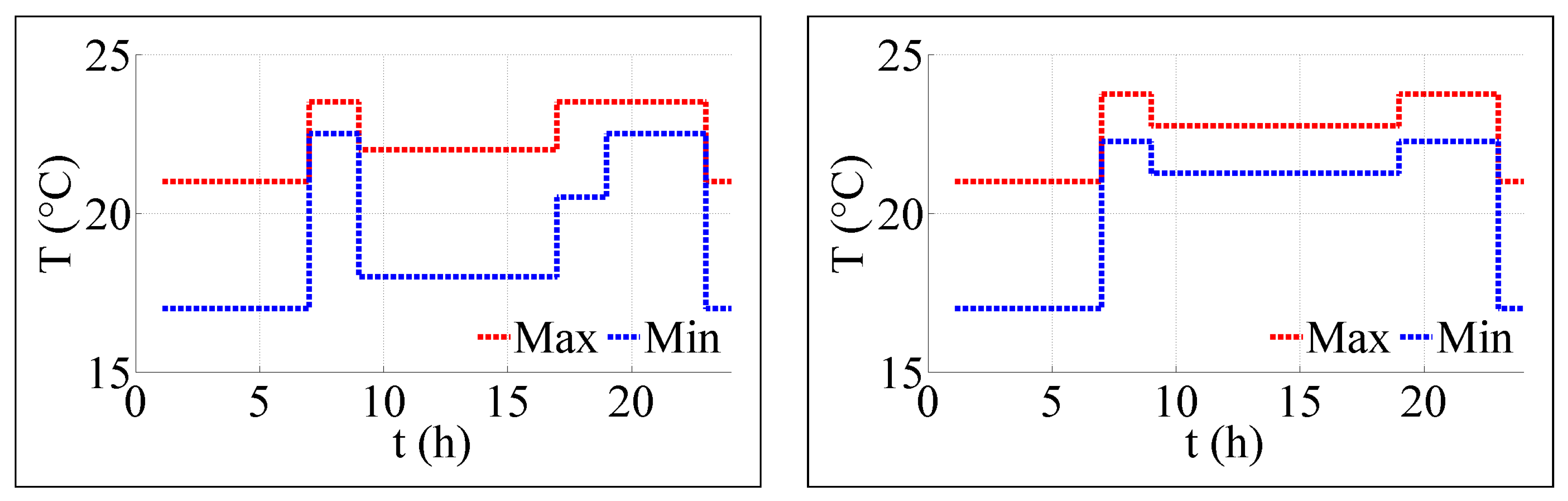
For each room and appliance h, the user is able to set the range of values between which the room temperature is to settle. Vectors ${\zeta }_h^{min}$ or ${\zeta }_h^{max}$ denote the minimum or maximum user-accepted room h temperature for all time slots t. Equation (20) defines this requirement formally. Without softening, the presented condition could result in the infeasibility of the optimization problem. However, by introducing variables $u_{h,t}^{min}$ and $u_{h,t}^{max}$ together with their minimization in the criteria function (23), the condition is softened, and the limits set by the user can be overstepped (yet at the expense of certain penalization in the criteria function). The slack variables matrices ${\mathbf{U}}^{min}$ and ${\mathbf{U}}^{max}$ always have to satisfy the condition (21).

$$\begin{array}{cc}{\zeta }_{h,t}^{min}-u_{h,t}^{min}\le T_{h,t}\le {\zeta }_{h,t}^{max}+u_{h,t}^{max}\hfill & \hfill \forall h,t\end{array}$$

(20)

$$\begin{array}{cc}{u}_{h,t}^{min}\ge 0,u_{h,t}^{max}\ge 0\hfill & \hfill \forall h,t\end{array}$$

(21)

$$\begin{array}{cc}0\le p_{h,t}\le P_{max,h}^{TC}\hfill & \hfill \forall h,t\end{array}$$

(22)

A finite output power of a TCA appliance can be described by constant $p_{h,t}^{TC}$ and must be less than the maximum output power $P_{max,h}$ (rule 22). Generally, a TCA is capable of both heating and cooling the given room. The simultaneous mode option (or the heating and cooling), namely, the configuration where it is possible to warm or cool based on the instantaneous difference of temperatures, has not found wide application in real conditions (the switching between the modes is usually performed twice a year only: during the spring and autumn periods) and, for this reason, is not discussed in this paper. The criteria function is as follows:

$$\begin{array}{cc}\hfill minJ(\Theta ,\Delta ,\mathit{P},{\mathit{u}}^{min},{\mathit{u}}^{max},w_{\Theta },w_{TH})=& \hfill \\ \hfill w_{\Theta }·\Delta ·\sum _{t=1}^T{\Theta }_t·\sum _{h=1}^{\left|\mathbb{H}\right|}{p}_{h,t}+w_{TH}& ·\sum _{t=1}^T\sum _{h=1}^{\left|\mathbb{H}\right|}\left({u_{h,t}^{min}}^2+{u_{h,t}^{max}}^2\right).\hfill \end{array}$$

(23)

3.4. Distributed Generators

This class of devices can be divided into two parts. The first subsection then comprises generators whose output power directly depends on the weather; thus, the generators are characterized by markedly limited controllability, and the energy production is predictable only with difficulty. In the second subsection, small micro-combined heat and power units ($\mu$CHP) are comprised; these devices produce electricity together with heat, which is then utilized as a source to heat or cool the building and to provide for warm water. Typical local generators include wind turbines, photovoltaic elements, solar thermal cells, and micro-combined heat and power units. In this paper, energy generation via wind turbines is considered.

Optimization models for systems with $\mu$CHP units are proposed within studies [33,34]. Thanks to their favorable cost and operating potential, cogeneration units are currently often employed to satisfy the heat and electricity requirements of multiple homes simultaneously; this option is analyzed in, for instance, study [31]. Further, sources [35,36] utilize wind speed prediction at the planning horizon to optimize energy production and transfer through wind generators; while the former paper assembles a MILP model to be resolved with an available solver, the latter one focuses on particle swarm optimization.

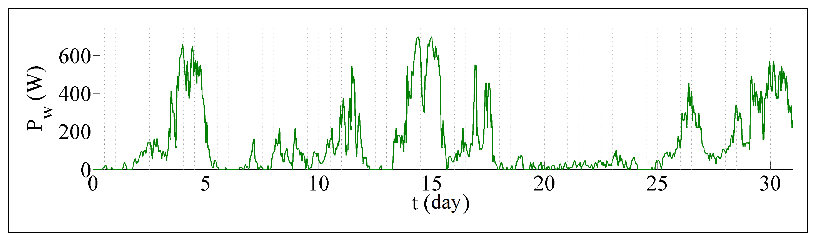
To ensure optimal use of the energy produced by a wind turbine, it is vital to possess a highly precise production estimate at the prediction horizon, and thus also an estimate of the wind flow velocity. The acquisition of such estimates is, due to the inhomogeneity of the atmosphere and constantly changing conditions, a complex and long-term problem analyzed systematically by meteorologists and mathematicians. An estimate of the future velocity of wind can be acquired either from an external source (weather forecast) or via compiling a probabilistic model based on historical data, as described in [37]. It is also possible to combine these two techniques, and such a procedure will enable us to use the probabilistic model for sufficiently accurate prediction to cover the first 4 h. The relationship between the generated energy volume and the velocity of wind is non-linear and depends on the concrete type of turbine and generator.

Before the actual optimization, the best prediction of the future values of wind flow velocity, $w_1\cdots w_T$, is determined in each time slot via applying the current data and the relevant historical model. The initial period of no more than first 3 h is defined through the most probable value from the model defined by Markov chains, and the rest of the planning horizon is predicted using publicly available mathematical model data. This technique, in spite of not being designed upon a solid scientific basis, provides very good results in real conditions [38].

$$\begin{array}{cc}{\mathbf{p}}_W^{RE}\left(t\right)=\left\{\begin{array}{cc}\Theta \left(v_{w,t}\right)& v_{\alpha }\le v_{w,t}\le v_{\beta }\\ P_n& v_{\beta }\le v_{w,t}\le v_{\gamma }\\ 0& otherwise\end{array}\right.\hfill & \hfill \forall t\in \langle 1\cdots T\rangle \end{array}$$

(24)

The amount of power generated by a turbine depends on the wind speed. The function describing this dependency is not linear (Equation (24)). For low wind speeds ($v_w\le v_{\alpha }$), the power is 0. The linear or quadratic relationship $\Theta \left(v_{w,t}\right)$ can be applied for medium speeds ($v_{\alpha }\le v_w\le v_{\beta }$). The maximum generated power is reached at high wind speeds ($v\beta \le v_w\le v_{\gamma }$). Above the value $v_{\gamma }$, the turbine must be stopped due to possible damage. The currently measured ($w_0$) and predicted ($w_1\cdots w_T$) values are, according to the above Expr. (24), used to calculate the vector ${\mathbf{P}}_W^{RE}$, whose individual elements then specify the predicted volume of energy produced by the wind turbine for the separate time slots on the planning horizon.

3.5. Accumulators

The integration of electromobile batteries into an energy management system is analyzed within references [39,40,41]; the benefits of connecting an electromobile are then discussed in detail by the authors of study [42]. In this context, let us note that energy storage within EMSs can be performed not only via batteries but also using other means, including, for example, fuel cells (as proposed in articles [43,44]). By extension, paper [45] outlines the connection of electric vehicles to the grid (V2G), and article [46] then examines, within the V2G problem, the planning of simultaneous charging in a large group of electromobiles from the perspective of cost optimization. Interestingly, study [47] describes the possibility of a large peak demand being generated during early night hours (namely, when large-scale charging of electromobiles is assumed); the paper also formulates a quadratic optimization problem to investigate different issues and economic benefits related to the various levels of the usage of electromobiles across the populace. The relevant paper [48] considers the stochastic character of the building energy management system; the introductory part of the study formulates the deterministic MILP. Further, a two-stage stochastic demand side management problem is created that addresses the stochastic nature of renewable energy generation, loads, EV availabilities, and EV energy demands.

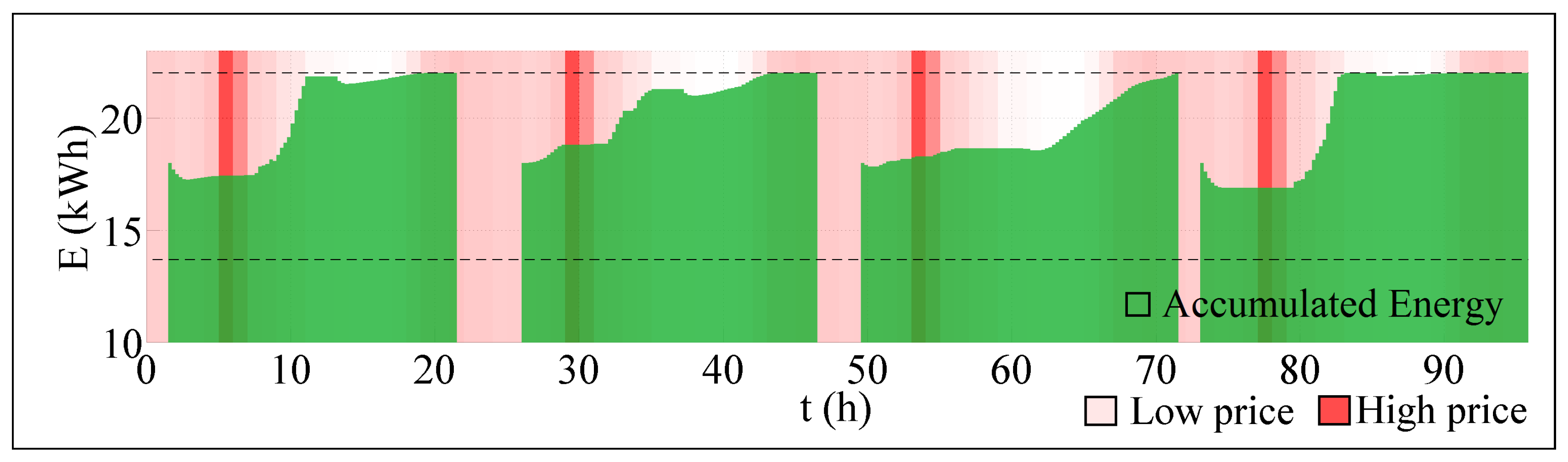
If the system comprises an accumulator, then energy can be taken off and stored at times of cheaper or easily available electricity and subsequently used whenever energy acquisition is expensive. Generally, it holds true that the higher the accumulator capacity, the wider the possibilites within the demand response system [39]; however, we also need to consider the relevant physical limitations, energy loss in time, and projected life of the accumulator.

Within the optimization problem, the battery condition is fully described by its remaining capacity in each time slot t, denoted as $q_t$. Due to the technical limitations of a concrete battery, this variable must lie within interval $\langle e_{min}^{ST},e_{max}^{ST}\rangle$ (Equation (25)). As follows from the relevant economic prospect [30], these two values may represent the battery discharge level corresponding to the maximum number of kilometers in a daily car trip and also the optimal charge level (which may amount to only 90% of energy due to the technical limitations of the given technology).

The energy remaining in the battery at the moment of the electromobile being connected to the system in time slot ${\alpha }^{ST}$ is denoted as $e_{\alpha }^{ST}$ (Equation (26)). By analogy, the desired energy in the battery after disconnection from the system in time slot ${\beta }^{ST}$ is expressed with $e_{\beta }^{ST}$ (Equation (27)). Outside the time interval represented by constants $\langle {\alpha }^{ST}$, ${\beta }^{ST}\rangle$, the battery remains disconnected (Equation (30)).

The energy volume charged into the battery in each time slot t is represented by the value of variable $c_t$; similarly, then, the discharged energy volume is denoted by the value of variable $d_t$. Equations (28) and (29) prevent the maximum energy volume charged during one time slot from exceeding $c_{max}^{ST}$ and, in the same sense, they ensure that the maximum discharged volume will not exceed $d_{max}^{ST}$.

$$\begin{array}{cc}0\le e_{min}^{ST}\le q_t\le e_{max}^{ST}\hfill & \hfill \forall t\end{array}$$

(25)

$$\begin{array}{c}{q}_{\alpha }^{ST}=e_{\alpha }^{ST}\hfill \end{array}$$

(26)

$$\begin{array}{c}{q}_{\beta }^{ST}=e_{\beta }^{ST}\hfill \end{array}$$

(27)

$$\begin{array}{cc}0\le c_t\le c_{max}^{ST}\hfill & \hfill \forall t\end{array}$$

(28)

$$\begin{array}{cc}0\le d_t\le d_{max}^{ST}\hfill & \hfill \forall t\end{array}$$

(29)

$$\begin{array}{cc}{c}_t=0,d_t=0\hfill & \hfill \forall t:t<{\alpha }^{ST}\vee t>{\beta }^{ST}\end{array}$$

(30)

The process of energy charging and discharging into/out of a battery, as described in Equation (31), is burdened with loss. Its efficiency is specified by constants ${\eta }_c$ for charging, or ${\eta }_d$ for discharging (${\eta }_c\in (0,1),{\eta }_d\in (0,1)$). Energy storage in a battery is accompanied by self-discharging; the proportional amount of energy drop in the battery during one time slot $\Delta$ is described by the constant $\kappa$ ($\kappa \to 0$). We have

$$\begin{array}{cc}{q}_t=q_{t-1}(1-\kappa )+\Delta \left(c_t{\eta }_c-\frac{d_t}{{\eta }_d}\right).\hfill & \hfill \forall t:{\alpha }^{ST}\le t\le {\beta }^{ST}\end{array}$$

(31)

The amortization to be considered for every 1 kWh of energy taken off the battery is denoted as ${\theta }_{unit}^{ST}$ and can be traced in the criteria function, which is further described in Section 4.

3.6. Energy Balance

The rules for modeling separate classes of home appliances have hitherto been defined separately; all these appliances nevertheless operate jointly within a single system, and they also consume shared electrical energy. In the mathematical model, this property is determined by the energy balance Equation (32). The left-hand side of the equation describes the total power taken off by a household, namely, the sum of the inputs of appliances included in the relevant categories (DE, IN, TH) and the input charged into the accumulator $c_t$ for the given time slot t; the right-hand side then specifies the supplied power. Here, the sum is that of the power taken off the accumulator, $d_t$; the power acquired via the generator from renewable resources, $p_t^{RE}$; and the power taken off the grid, $p_t^{MAINS}$, in the same time slot. The relaxation variable $u_t^{MAINS}$ ensures the feasibility of the entire optimization problem. We have

$$\begin{array}{cc}\sum _{a=1}^{\mathbb{A}}{p}_{a,t}^{DE}+\sum _{i=1}^{\mathbb{I}}{e}_i^{IN}+\sum _{h=1}^{\mathbb{H}}{p}_{h,t}^{TH}+c_t=p_t^{RE}+d_t+p_t^{MAINS}\hfill & \hfill \forall t\end{array}$$

(32)

$$\begin{array}{cc}0\le p_t^{MAINS}\le P_{MAX}^{MAINS}+u_t^{MAINS}\hfill & \hfill \forall t\end{array}$$

(33)

$$\begin{array}{cc}{u}_t^{MAINS}\ge 0.\hfill & \hfill \forall t\end{array}$$

(34)

4. Optimization Problem

For EMSs, this paper defines a mixed integer quadratic problem (MIQP) consisting of the following elements: the rules and bounds for individual appliances defined within previous chapters; global technical and other restrictions (such as energy balance); and criteria function, whose shape corresponds to the selected strategy. For this article, we chose several requirements specified in [30]; these requirements and the resulting control strategy are described below.

4.1. Price Minimization

The basic end user requirement addressed at the demand response system is to reduce the relevant cost. The expression ${\Psi }_{\Theta }$ in function (39) indicates the total cost of energy consumed by all appliance categories for the entire prediction horizon. This price is obtained as the product of the unit price in time slot ${\Theta }_t$ and the energy taken off the grid in individual time slots (96 intervals, each 15 min long). For each time slot, the extracted energy is calculated as the sum of the following components: the energy consumed by deferrable (DE, Equation (35)), interruptible (IN, Equation (36)), and thermostatically controlled (TH, Equation (37)) appliances; the energy charged into the accumulator; the negatively assumed value of energy discharged from the accumulator (Equation (38)); and the values of energy produced by the wind turbine $p_t^{RE}$.

$$\begin{array}{c}{\psi }_t^{DE}=\sum _{a=1}^{\left|\mathbb{A}\right|}\sum _{j=1}^{l_a^{DE}}{r}_{a,t-j+1}{e}_{a,t}^{DE}\hfill \end{array}$$

(35)

$$\begin{array}{c}{\psi }_t^{IN}=\sum _{i=1}^{\left|\mathbb{I}\right|}\Delta ·e_i^{IN}·m_{i,t}\hfill \end{array}$$

(36)

$$\begin{array}{c}{\psi }_t^{TH}=\sum _{h=1}^{\left|\mathbb{H}\right|}\Delta ·p_{h,t}^{TH}\hfill \end{array}$$

(37)

$$\begin{array}{c}{\psi }_t^{ST}=c_t-d_t\hfill \end{array}$$

(38)

$$\begin{array}{c}{\Psi }_{\Theta }=\sum _{t=1}^T{\Theta }_t·\left({\psi }_t^{DE}+{\psi }_t^{IN}+{\psi }_t^{TH}+{\psi }_t^{ST}-\Delta ·p_t^{RE}\right)\hfill \end{array}$$

(39)

4.2. Observation of Preferred Times to Run DE Appliances

The minimization of Equation (40) leads to such system behavior in which the working cycle of deferrable appliances is executed as early as possible within the user-selected interval.

In Real-time pricing (RTP) tariffs, where it is necessary to rely significantly on the prediction of future energy prices (as described by, for example, [49]), the combination of the requirements for observing the preferred times and minimizing the price eventually reduces the risk of wrong price estimation. The prediction reliability is generally highest at the beginning of the predicted interval and gradually decreases into the future. In simple words, shifting the appliance cycle far into the future is not beneficial, because the corresponding price is predicted with only low probability.

While this paper does not consider RTP tariffs, minimizing the criteria function below does not provide any value added for this study; however, we present the relevant formula to demonstrate the ability of the optimization algorithm. We have

$$\begin{array}{c}{\Psi }_{DE}=\frac{1}{\left|\mathbb{A}\right|}\sum _{a\in \mathbb{A}}\left(s_a-{\alpha }_a\right).\hfill \end{array}$$

(40)

4.3. Maximization of Thermal Comfort

The minimization of Equation (41) ensures the observance of optimal temperature patterns in individual rooms (maximizes the thermal comfort) because it penalizes higher values of slack variables ${\mathbf{u}}^{min}$ and ${\mathbf{u}}^{max}$, which constitute the difference between the real temperature and the minimum/maximum temperature desired by the user under simultaneous adherence to the restricting conditions for a concrete device. The optimum solution of this equation leads to maintaining the temperature at the mean value between the minimum and maximum limits within the entire planning horizon:

$$\begin{array}{c}{\Psi }_{TH}=\frac{1}{\left|\mathbb{H}\right|}\sum _{t=1}^T\sum _{h\in \mathbb{H}}\left({u_{h,t}^{min}}^2+{u_{h,t}^{max}}^2\right).\hfill \end{array}$$

(41)

4.4. Minimizing the Frequency of Control Actions

In cases when a control action in thermostatically controlled appliances is changed via an electromechanical element (such as a servo drive), it appears suitable that the controller minimize the frequency of desired control actions. To satisfy such a condition, we can either add rules which will ensure the equality of control actions always in several neighboring action slots or adjust the criteria function. For simplicity, this paper utilizes the method of modifying the said function by adding Equation (42), which is to guarantee the minimization of the difference between control actions always in two neighboring time slots. We define

$$\begin{array}{c}{\Psi }_{TH,P}=\sum _{h=1}^{\mathbb{H}}\sum _{t=2}^T{\left(p_{h,t}-p_{h,t-1}\right)}^2.\hfill \end{array}$$

(42)

4.5. Multicriteria Optimization and the Heuristic Algorithm

During multicriteria optimization, the setting of preferences (weights of individual members) constitutes a key problem, especially because each of the variables ${\Psi }_{\Theta }$, ${\Psi }_{DE}$, ${\Psi }_{TH}$, and ${\Psi }_{TH,P}$ may assume different values, and these may differ by up to several orders. At the same time, however, the magnitudes of the variables change substantially in individual control cycles with receding horizon.

If, in optimization, the setting of the weights of particular members is to be meaningful, we have to ensure that individual variables assume only values within certain limits. Thus, it is necessary to establish the presumed lowest and highest values of each of the variables and perform normalization, which will not only approximately unify (within an order) the values of the variables but also compensate for their large variations during the run of the system.

The limits ${\Psi }^{min}$ and ${\Psi }^{max}$ of individual variables thus have to be determined before each optimization process, always on the basis of actual input parameters. In this paper, a heuristic algorithm to calculate the said limits is presented. This algorithm has to be invariably triggered with current parameters before the optimization of the model within a new time slot. The algorithm determines the price limits related to the consumed energy (${\Psi }_{\Theta }$ for individual appliance classes: ${\Psi }_{\Theta ,DE}$, ${\Psi }_{\Theta ,IN}$, ${\Psi }_{\Theta ,TH}$ and ${\Psi }_{\Theta ,ST}$), the range of variables ${\Psi }_{DE}$ and ${\Psi }_{TH}$ for determining the comfort of devices DE and TH, and the range of variable ${\Psi }_{TH,P}$ for restricting the magnitude of the control action of TH appliances.

• In deferrable appliances, the procedure of determining the lower limit ${\Psi }_{\Theta ,DE}^{min}$ involves a simple search of such positioning of the device within the user-preferred interval that will ensure the lowest price of the consumed energy. The upper limit ${\Psi }_{\Theta ,DE}^{max}$ is then determined as the average of several random simulated runs of the appliance within the said interval.
• The discussed procedure in interruptible appliances is trivial only if no additional rules are defined for their run (Equations (10)–(12)). In such a case, the lower limit ${\Psi }_{\Theta ,IN}^{min}$ is calculated with positioning the appliance cycles into the time slots that exhibit the lowest price, and the upper limit ${\Psi }_{\Theta ,IN}^{max}$ is then established as the average price for several random cycle positions. As regards the situation where further rules are defined for the running of interruptible appliances, a detailed description is available in [30].
• In thermostatically controlled appliances, the upper limit ${\Psi }_{\Theta ,TH}^{max}$ is determined by the algorithm, which simulates a simple two-state regulator on the prediction horizon. The lower limit ${\Psi }_{\Theta ,TH}^{min}$ is then established via calculation as a proportional part of the upper limit or based on the results of previous optimizations.
• The boundaries for the index of comfort violation in deferrable appliances, ${\Psi }_{DE}^{min}$ or ${\Psi }_{DE}^{max}$, can be easily determined from the knowledge of the user-preferred time window to run the appliance. If no explicit definition of the preferred time window is available, we can use its beginning or, possibly, a half of the whole interval. The limits of the other variables, such as the comfort violation levels ${\Psi }_{TH}$ and ${\Psi }_{TH,P}$, are obtained based on empirically defined input parameters.

After establishing the above-presented parameters, individual variables in the criteria function can be normalized according to formulas (43)–(46). We have

$$\begin{array}{c}{\overline{\Psi }}_{\Theta }=\frac{{\Psi }_{\Theta }-{\Psi }_{\Theta }^{min}}{{\Psi }_{\Theta }^{max}-{\Psi }_{\Theta }^{min}}\hfill \end{array}$$

(43)

$$\begin{array}{c}{\overline{\Psi }}_{DE}=\frac{{\Psi }_{DE}-{\Psi }_{DE}^{min}}{{\Psi }_{DE}^{max}-{\Psi }_{DE}^{min}}\hfill \end{array}$$

(44)

$$\begin{array}{c}{\overline{\Psi }}_{TH}=\frac{{\Psi }_{TH}-{\Psi }_{TH}^{min}}{{\Psi }_{TH}^{max}-{\Psi }_{TH}^{min}}\hfill \end{array}$$

(45)

$$\begin{array}{c}{\overline{\Psi }}_{TH,P}=\frac{{\Psi }_{TH,P}-{\Psi }_{TH,P}^{min}}{{\Psi }_{TH,P}^{max}-{\Psi }_{TH,P}^{min}}\hfill \end{array}$$

(46)

$$\begin{array}{c}{\overline{\Psi }}_{PP}={\Psi }_{PP}.\hfill \end{array}$$

(47)

4.6. Weight Setting

Upon user decision, each of the specified criteria, ${\overline{\Psi }}_{\Theta }(·)$, ${\overline{\Psi }}_{DE}(·)$, ${\overline{\Psi }}_{TH}(·)$, and ${\overline{\Psi }}_{TH,P}(·)$, is assigned a weight w, which then decides on the relative importance of the given criterion. While cost-conscious users accentuate price minimization, and thus a higher weight has to be allocated to this objective, those preferring thermal comfort naturally behave in a different manner. Optimization therefore enables us to set all the criteria in the required balance, and some of them can also be excluded from the calculation by assigning zero value to the corresponding weights. The resulting criteria function for the energy manager then corresponds to the sum of individual weighted variables, and the whole optimization task is formally defined as

$$\begin{array}{c}\mathrm{minimize}{\omega }_{\Theta }·{\overline{\Psi }}_{\Theta }+{\omega }_{DE}·{\overline{\Psi }}_{DE}+{\omega }_{TH}·{\overline{\Psi }}_{TH}+{\omega }_{TH,P}·{\overline{\Psi }}_{TH,P}+{\overline{\Psi }}_{PP}\hfill \\ \mathrm{based}\mathrm{on}\mathrm{rules}\left(3\right)–\left(34\right).\hfill \end{array}$$

(48)

Due to the normalization described within the last subsection, we can set the individual weighting coefficients as indicated below:

$$\begin{array}{c}\hfill \sum \left({\omega }_{\Theta }+{\omega }_{DE}+{\omega }_{TH}+{\omega }_{TH,P}\right)=1.\end{array}$$

(49)

The optimization problem solution can be found using algorithms specialized in searching a solution to combinatorial optimization problems. In this paper, the CPLEX solver [50] is exploited as a tool to effectively compute the overall optimization problem solution.

5. Case Study

To verify the functionality of the proposed method, we use in this section a concrete mathematical model of a system for all types of appliances.

5.1. Building Energy Management Model

Within this section, we define five groups of appliances, corresponding to the classification introduced previously in Section 3.

5.1.1. Deferrable Appliances

We modeled three deferrable appliances: a washing machine (WM), a dishwasher (DW), and a tumble dryer (TD). According to source [51], we determined the average number of cycles per year to obtain the probability of running a specific appliance during a specific simulation day (

Table 1. The average number of cycles for specific DE appliances.

Appliance	Cycles Per Year	Probability for a Concrete Day
WM	220	0.6023
DW	240	0.6570
TD	147	0.4024

). The energy consumption and peak power cycles were yielded through a measurement of real appliances. Relevant examples are shown in Figure 1. The user preferences for a particular appliances’ schedule are summarized within

Table 2. The user preferences for the related DE appliances’ schedule.

Appliance	Earliest Start Time Slot	Latest End Time Slot
WM	$X_{WM,s}^{DE}\sim \mathcal{U}(24,48)$	$X_{WM,f}^{DE}\sim \mathcal{U}(60,80)$
DW	$X_{DW,s}^{DE}\sim \mathcal{U}(16,40)$	$X_{DW,f}^{DE}\sim \mathcal{U}(60,80)$
TD	$X_{TD,s}^{DE}\sim \mathcal{U}(24,48)$	$X_{TD,f}^{DE}\sim \mathcal{U}(50,80)$

(the earliest start and latest end of an appliance cycle for a simulation day are uniformly distributed values).

5.1.2. Interruptible Appliances

We modeled two interruptible appliances: a pool pump (PP) and an electric water heater (EWH).

Table 3. The parameters of the IN appliances.

Appliance	Power (W)	Power Cycle Length (h)	Restrictions
PP	300	5	2 slots
EWH	2200	3.5	-

summarizes all the necessary parameters for these appliances. Both the devices are scheduled for all the simulation days. The restriction for scheduling a specific appliance only during particular time slots was not applied in this case study.

5.1.3. Thermostatically Controlled Appliances

We used a simplified model of a building with 4 equally large rooms [30]; for simplicity, no windows are considered. Moreover, only the thermal conduction principle is used to exchange thermal energy between the rooms. An electrical heating unit (2350 watts of input power) is employed to heat each room. The inner dynamics of the unit are neglected as they are significantly faster than the building thermal dynamics. The system of differential equations corresponds to the equivalent electrical circuit described in [30].

Table 4. The physical parameters of the particular rooms.

Room	V$\left({\mathit{m}}^3\right)$	${\mathit{c}}_{\mathit{r}}$$\left(\frac{\mathit{kJ}}{\mathit{kg}·\mathit{K}}\right)$	$\mathit{\lambda }$$\left(\frac{\mathit{W}}{\mathit{m}·\mathit{K}}\right)$	$\mathit{\rho }$$\left(\frac{\mathit{kg}}{{\mathit{m}}^3}\right)$
$r_1$, $r_2$, $r_3$, $r_4$	62.5	$c_a$	0.0252	1.188

describes the physical parameters of the particular rooms, while

Table 5. The physical parameters of the particular walls.

Wall	d$\left(\mathit{m}\right)$	S$\left({\mathit{m}}^2\right)$	c$\left(\frac{\mathit{kJ}}{\mathit{kg}·{\mathit{K}}^{-1}}\right)$	$\mathit{\lambda }$$\left(\frac{\mathit{W}}{\mathit{m}·\mathit{K}}\right)$	$\mathit{\rho }$$\left(\frac{\mathit{kg}}{{\mathit{m}}^3}\right)$
$w_1$, $w_3$, $w_5$, $w_7$	0.375	25.0	1000	0.150	850
$w_2$, $w_4$, $w_6$, $w_8$	0.100	12.5	1000	0.170	700

characterizes the physical parameters of the walls. The thermal transmittance values $h_{in}$ and $h_{out}$ are selected to be $7.6923$, and 25, respectively. The thermal power of each heating unit is 1170 watts, the corresponding hot air volume amounts to 106 m${}^3·$h${}^{-1}$, and the temperature equals 43 °C.

For the first stage of the simulation, the initial values for all the room temperatures are set to a half of the interval specified by the user setpoints. The temperature of the walls is set to a half of the temperature difference between neighboring rooms, or a half of the temperature difference between the room and the ambient temperature.

For clarity, the user setpoints are equal for all the rooms and throughout the simulation. The setpoints for a regular weekday are shown in Figure 2 on the left-hand side, whereas the setpoints for the weekend are available on the right-hand side.

5.1.4. Accumulators

In this case study, we model an accumulator used in a Nissan Leaf EV. A detailed description of this accumulator and its technical parameters is provided in reference [52]. The first and last time slots to connect or disconnect the accumulator in the EMS are characterized as uniformly distributed random variables $X_c^{ST}\sim \mathcal{U}(20,32)$ and $X_d^{ST}\sim \mathcal{U}(60,76)$, respectively, for each day. The amount of kilometers driven by the EV before its connection to the system is computed as $X_{range}^{ST}\sim \mathcal{N}(40,100)$ for each day.

5.1.5. Wind Turbine

The wind energy generation problem comprises two parts. The probabilistic model adopted from paper [53] was constructed based on historical wind speed measurements at Brno Airport (LKTB) between the years of 2004 and 2014. All the values are handled as follows: The fractional parts are cut and the values branched into categories; for each hour of the day, there are categories according to the wind speed, namely, (0 m·s${}^{-1}$, 1 m·s${}^{-1}$], (1 m·s${}^{-1}$, 2 m·s${}^{-1}$], ..., ($n-1$ m·s${}^{-1}$, $n$m·s${}^{-1}$]. Each of these describes the number of the occurrences of a particular wind speed at a particular hour of the day. For each hour k, the first order Markov Chain with transition matrix $P_k$ is created. The elements $(i,j)$ of this matrix then characterize the probability that the wind speed i m·s${}^{-1}$ will change to the value j m·s${}^{-1}$ during the hour k. More details of the probabilistic model are defined in study [30]. For the simulation, we selected a three blade wind turbine with the diameter of 2.5 m for the nominal wind speed 8 m·s${}^{-1}$ (detailed information is available in [54]).

5.1.6. Other Simulation Parameters

To simulate the system behavior, a winter period (November 2014–January 2015) was considered. The ambient temperature (Figure 3) was adopted from source [55]. The model is influenced by not only the ambient temperature but also the wind speed. Based on the parameters described within Section 5.1.5, we calculated the expected power to be generated through the wind turbine. The computed values for the first simulation month are available in Figure 4.

5.2. Results

The case study contains two interconnected parts. While the former section verifies the functionality of the complete proposed model, the latter one responds to the question of how it is possible to simulate various user preferences (reduced costs—timely triggering of appliances—maintenance of thermal comfort & technical aspects) by tuning the individual parameters of the optimization function; the above-outlined user settings are then used to describe differences in the system behavior. Thus, the heuristic algorithm functionality is verified to facilitate the estimation of the limits of the criteria function variables.

The study encompasses a period of three months, during which we simulate the use of home appliances according to preassigned parameters over weekdays, weekends, and holidays (this being a time when the users are not present in the monitored homes). Based on the type of day, the actual manner of running the individual appliances progressively changes.

For each simulated day, the data are processed by means of the heuristic algorithm to calculate the normalization coefficients. The mean values of the coefficients are summarized in the corresponding

Table 6. The normalization coefficients calculated by the heuristic algorithm.

Appliances	Type	Symbol	Minimal ${\mathbf{\Psi }}_{\diamond }^{\mathit{min}}$	Maximal ${\mathbf{\Psi }}_{\diamond }^{\mathit{max}}$
DE	Price	${\Psi }_{\Theta ,DE}$	0	11.41
DE	Comfort	${\Psi }_{DE}$	0	732.5
TCA	Price	${\Psi }_{\Theta ,TH}$	19.61	69.15
TCA	Comfort	${\Psi }_{TH}$	0	16
TCA	Control action	${\Psi }_{TH,P}$	2.788 × 10${}^{-3}$	2.788 × 10${}^{-2}$
IN	Price	${\Psi }_{\Theta ,IN}$	3.58	30.32
ST	Price	${\Psi }_{\Theta ,ST}$	0	31.58

, and Figure 5 then shows the graphically represented values for the individual components of the total cost (each concrete color field denotes, for separate days, the lowest ${\Psi }_{\diamond }^{min}$ and highest ${\Psi }_{\diamond }^{max}$ values for concrete appliance types. Thus, for instance, the first simulated day shows the difference between the minimum and maximum prices for the TCAs ${\Psi }_{\Theta }^{DE}$ amounting to 31 CZK.

The diagram in Figure 5 indicates the evolution of the lowest and highest values of the individual cost components during the simulation interval. Here, it becomes obvious that, while the cost of operating thermostatically controlled appliances remains (excepting the holiday) without major differences throughout the entire interval, the cost of operating deferrable appliances is markedly volatile, depending on which appliances are triggered and run during a concrete day. Generally, the price fluctuation would not constitute an essential problem if absolute values for the other normalization coefficients did not differ by up to several orders, as outlined in Table 6. The optimization function specified as Equation (48) therefore must comprise the normalized values obtained by substituting the calculated coefficients ${\Psi }_{\diamond }^{min}$ a ${\Psi }_{\diamond }^{max}$ into the expressions in Equations (43)–(46).

After normalization, the individual members of the optimization function can be weighted via multiplication by the constants. This action enables emphasizing or suppressing the significance of the cost reduction (${\omega }_{\Theta }$), preferred running interval of deferrable appliances (${\omega }_{DE}$), maintenance of thermal comfort (${\omega }_{TH}$), and reduction of the magnitude and frequency of control action in thermostatically controlled appliances (${\omega }_{TH,P}$).

5.3. Verification of the System Model

In this section, we simulate the system behavior with the weights set to ${\omega }_{\Theta }=0.33$, ${\omega }_{DE}=0.33$, ${\omega }_{TH}=0.33$, and ${\omega }_{TH,P}=0.01$. Figure 6 indicates the cost of running the individual types of appliances during the simulated period. As regards the days on which the values of the diagram start from the negative section of the price axis ${\Theta }_t$, the local generator supplied the system with energy at a corresponding cost, and the total bill is thus reduced by this amount. The diagram shows a marked drop of cost in interruptible appliances and accumulator charging between the 30th and 40th days defined within the input conditions. Although the said days involved also reduction of the desired temperature in the building, this fact did not visually reflect in the cost of energy for thermostatically controlled appliances; such behavior can be attributed to the lower outer temperature during the monitored period, and thus the difference between the outer and inner desired temperatures was approximately the same as in other periods of simulation.

Figure 7 then presents, for the entire simulated period, the resulting values of the individual parts of the criterion after the end of the optimization. It is obvious from this figure that the values correspond to the input requirements given by the individual weights: the first three values (${\overline{\Psi }}_{\Theta }$, ${\overline{\Psi }}_{DE}$, and ${\overline{\Psi }}_{TH}$), roughly oscillate between 0 and 1, while the last one, (${\overline{\Psi }}_{TH,P}$), whose weight was markedly lower, reached multiply higher levels. We can also notice that the values are not strictly enclosed in the above interval, and thus, for example, the price criterion values (${\overline{\Psi }}_{\Theta }$) assume also a negative character. This is given by both the design of the heuristic algorithm and the fact that the calculated values constitute only estimates of the upper and lower limits of the individual values. Such behavior, however, is not a difficulty.

The operation of separate appliances within the first four simulation days is shown in Figure 8, Figure 9 and Figure 10. For all the figures, the deepness of the red in the background corresponds to the energy price fluctuation in time (the deeper the color, the more expensive the energy for the time slot). The first of the figures referred to above, Figure 8, describes the activity of interruptible (patterns WM, DW, TD) and deferrable (patterns PP, EWH) appliances. In the diagram, the gray tinge indicates the user preferences, or the allowed run intervals in separate appliances. Even though the scheduling of these intervals may appear flawed because some appliances are run at times when the cost of energy stands at the highest level, Figure 11 informs us that the power needed for the actual triggering was not taken off the grid but acquired from an accumulator or a local energy source.

Figure 9 displays the behavior of temperatures in separate spaces. For simplicity, we chose the same patterns for all four rooms involved, and as these rooms and the relationships between them are modeled identically, we also obtain identical optimal patterns of the desired values.

Figure 10 then shows the optimal behavior of residual energy in the accumulator for each day between its connection (accumulator discharged, start of the green block) and disconnection (accumulator charged, end of the green block). The connection and disconnection times, as well as the residual capacity at connection and the desired capacity at disconnection, are given by the input conditions.

The figure below (Figure 11) presents the balance between the energy input and output during the first four days of simulation, and it captures the expected optimal behavior of the system in time. The negative section of the diagram relates to the power supplied to the system, and the concrete power sources are as follows: the black path determines the power taken off the distribution grid (limited to the value of 3850 W indicated via the dashed line; the green path indicates the output provided by the accumulator; and the yellow one defines the predicated output supplied by the local generator. The positive values represent the inputs of the individual appliance classes, namely, the deferrable (violet), interruptible (cyan), and thermostatically controlled (blue) groups. The power loaded in the accumulator is then displayed with the red path. The sum of the outputs in each time slot equals zero.

The text above summarizes the results obtained for one concrete setting of the weights of the criteria function members. The presented diagrams were outlined to provide the simplest possible view of the functionality of the model of the entire system; the correct functioning of the model for EMSs was verified via the testing and detailed analysis of both the patterns and the numerical results.

5.4. Heuristic Algorithm Validation

As we have already pointed out, multicriteria optimization was used in several studies published previously; however, in all these papers it was necessary to set experimentally the weights of the members in the optimization function. The said drawback is effectively solved via applying the heuristic algorithm; then, based on the obtained result, the optimization function members can be simply weighted.

This chapter describes four optimization cases to which there correspond four members in the optimization function and four different weighting variables. The actual testing was performed such that for each of the weights ${\omega }_{\diamond }$ we progressively set the values 0, 0.01, 0.1, 0.2,⋯,0.8, 0.9, 0.99, 1, and the other weights ${\omega }_{⧫}$ were invariably assigned values according to the formula ${\omega }_{⧫}=\frac{1}{3}·(1-{\omega }_{\diamond })$.

5.4.1. Price Preference

Figure 12 displays the patterns of the individual optimization function members. The member ${\overline{\Psi }}_{\Theta }$ represents the gradually decreasing price in relation to its increasing preference ${\omega }_{\Theta }$. It becomes obvious that as soon as we have ${\omega }_{\Theta }=0$, the price is not included in the optimization function and thus exhibits a high value (the vertical axis of the diagram has a logarithmic scale). With the progressive price preference growth, the price decreases at the expense of the other three properties of the system. At the moment when the weight ${\omega }_{\Theta }=1$ is set, the price is optimized regardless of the values of the other members, and the cost specification for this variant is missing in the logarithmic diagram because the calculation here yields a small negative value (the negative value of the member does not constitute a problem: it only refers to the fact that the heuristic normalization algorithm did not calculate the minimum value precisely. In this case, at ${\omega }_{\Theta }=1$, the system reaches a state when (for example) TCA appliances are not triggered at all, a condition for which the algorithm is not designed). The values of the other three members then increase abruptly.

5.4.2. Preference of the Deferrable Appliances Comfort

The results of this option are presented in Figure 13. The first sight reveals that a change of the weight ${\omega }_{DE}$ does not markedly affect the behavior of the system in the given case; this is caused by a favorable combination of the time behavior of the energy price, the user preferences in deferrable appliances, and the fact that the discussed member is not too closely connected with the other members considered. Thus, during optimization, it is not difficult to set up an optimal value of the member ${\overline{\Psi }}_{DE}$ to obtain an optimal solution. In an extreme case, ${\omega }_{DE}=1$, the other members of the criteria function are weighted by the value of 0 (the price member ${\overline{\Psi }}_{\Theta }$ in particular), a large number of the model parts are not applied, and the optimization process generates incorrect results.

5.4.3. Thermal Comfort Preference

The variation of the system behavior based on a weight change in the thermal comfort member ${\omega }_{TH}$ is shown in Figure 14. The model behavior becomes extreme also in cases ${\omega }_{TH}=0$ and ${\omega }_{TH}=1$. As regards the former case, then again no triggering of thermostatically controlled appliances occurs: the normalized member for price minimization, ${\overline{\Psi }}_{\Theta }$, equals 0, in the same manner as the member to minimize the control action for TCA ${\overline{\Psi }}_{TH,P}$ (which is a logical condition, given the fact that the said member is defined in the criteria function as a sum of the output differences characterizing the TCA appliances in the adjacent time slots). With the growing weight of ${\omega }_{TH}$, we can observe a gradual decrease of the member ${\overline{\Psi }}_{TH}$, meaning an improvement in the quality of the thermal comfort within the building. However, excessive suppression of the other weights (${\omega }_{TH}>0.9$) affects the magnitude of the other members: the optimization algorithm is not forced to minimize their sizes, and again the system behaves incorrectly.

5.4.4. Preference of Reducing the Control Action of TCA

The pattern of the values of the individual members of the optimization function at various weight levels, ${\omega }_{TH,P}$, is presented in Figure 15. As its magnitude grows, the value of this weight becomes an influence on “softening” the alteration of the control action for TCAs. This characteristic then manifests itself especially via a decrease of thermal comfort, in which—assuming this concrete case—the system is not capable of reacting to fast demand changes. In the case of ${\omega }_{TH,P}=0$, the member ${\overline{\Psi }}_{TH,P}$ is ignored, and the control action is not modified in any manner. The opposite condition, ${\omega }_{TH,P}=1$, again involves the suppression of the weights of the other criteria function members, which then reflects in a rapid increase of their values, and the system ceases to function as required.

6. Evaluation and Conclusions

The above-presented scenarios indicate how the behavior of the system changes under variation of the constants weighting individual members of the criteria function. Generally, the investigation of the discussed cases and patterns allows us to formulate the following points:

• As the individual members of the optimization function are normalized using values obtained through applying the heuristic algorithm, it is possible to influence the system behavior comprehensively via multiplying the normalized members by weighting coefficients within the range of between 0 and 1. The sum of all weighting coefficients may equal 1, but this does not constitute a necessary precondition. However, if the weighting coefficients were set directly by the user over the corresponding system interface, the sum of the individual request weights equal to 1 (or 100%) would retain in the user an awareness of the quid pro quo principle.
• Setting any of the weights to the value of 0 or 1 would lead to its complete omission or one-sided preference; however, the technique of defining the optimization problem is not ready for such a scenario, and the results are unusable. For this reason, the discussed type of setting has to be avoided to preclude unnecessary difficulties.

This work presents a design of a universal method for optimal electricity consumption planning in a smart home. The technique was validated via software implementation. We considered not only home appliances but also local electricity sources, and these entities were classified into five categories (according to their typical use and related properties) as follows: devices with deferrable and uninterruptible cycles; interruptible cycle appliances; thermostatically controlled devices; accumulators and local generators operating on the basis of renewable sources. Each of the categories was subsequently complemented with a relevant mathematical model. By extension, the article also partly considers the problem of non-controllable appliances. The proposed method enables the end user to utilize the demand response principle in optimizing the cost of consumed electricity. In view of the above facts, it is important to note that the concept introduced herein assumes the inclusion of an energy manager, namely, a tool to coordinate the triggering of individual smart home appliances based on a series of input data, including information acquired from the distributor’s infrastructure. An energy manager is a comprehensive instrument for maintaining a mathematical model synthetized from models of separate appliances, and this instrument also secures the implementation of the method designed to resolve the complex optimization problem. The basic purpose of the manager consists in ensuring cost reduction at the level of appliance operation comfort adopted by the user. Significantly, the discussed tool is also capable of respecting the technical limitations of the individual devices. Within this paper, we solve a part of the above-defined task, which relates to optimizing the run of appliances in a single home. The solution of the optimization task consists in minimizing the quadratic function formed by a weighted sum of partial functions representing individual demands with respect to linear bounds, namely, the function defined for separate appliances and also user preferences (the problem is therefore one of mixed integer quadratic programming). Considering the fact that the requirements are often contradictory, the optimization task solution falls within the set of multicriteria combinatorial problems. By changing the values of the weighting constants of the individual parts of the criteria function, we can then emphasize or suppress a certain behavioral aspect.

The proposed method, extended with the heuristic algorithm, was validated using a pair of universal software tools: Matlab (MathWorks, Massachusetts, United States) and CPLEX (IBM, New York, United States) Optimization Studio. While the former toolkit enabled us to generate the input parameters and present the results, the latter one ensured the solution of the actual optimization task. Within the research related to this paper, we also created a software simulation tool to model the behavior of a group of deferrable cycle appliances on a receding horizon. This tool was compiled as a contribution to project FP7-ARTEMIS (333020-ACCUS-Adaptive Cooperative Control in Urban Subsystems). Using the described software, we then carried out several case studies facilitating the verification of the desired properties of the system.

The implementation of the above-specified technique into a device coordinating the run of appliances in a smart home system will enable us to materialize the demand response principle; thus, the system will be capable of swiftly reacting to a change in the input conditions by adjusting the electricity consumption rate. Importantly, the case study has shown that the proposed solution satisfies the conditions stipulated within the underlying research presented via this paper.

References

1. Mohsenian-Rad, A.H.; Leon-Garcia, A. Optimal Residential Load Control With Price Prediction in Real-Time Electricity Pricing Environments. IEEE Trans. Smart Grid 2010, 1, 120–133. [Google Scholar] [CrossRef]
2. Braithwait, S.D. Real-Time Pricing and Demand Response Can Work within Limits. Nat. Gas Electr. 2005, 21, 1–31. [Google Scholar]
3. Soares, J.; Canizes, B.; Lobo, C.; Vale, Z.; Morais, H. Electric Vehicle Scenario Simulator Tool for Smart Grid Operators. Energies 2012, 5, 1881–1899. [Google Scholar] [CrossRef]
4. LeMay, M.; Nelli, R.; Gross, G.; Gunter, C. An Integrated Architecture for Demand Response Communications and Control. In Proceedings of the 41st Annual Hawaii International Conference on System Sciences, Big Island, HI, USA, 7–10 January 2008; p. 174. [Google Scholar]
5. Widén, J.; Wäckelgard, E. A high-resolution stochastic model of domestic activity patterns and electricity demand. Appl. Energy 2010, 87, 1880–1892. [Google Scholar] [CrossRef]
6. Zhu, Z.; Tang, J.; Lambotharan, S.; Chin, W.H.; Fan, Z. An integer linear programming based optimization for home demand-side management in smart grid. In Proceedings of the IEEE PES Innovative Smart Grid Technologies (ISGT), Washington, DC, USA, 16–20 January 2012; pp. 1–5. [Google Scholar]
7. Gottwalt, S.; Ketter, W.; Block, C.; Collins, J.; Weinhardt, C. Demand side management: A simulation of household behavior under variable prices. Energy Policy 2011, 39, 8163–8174. [Google Scholar] [CrossRef]
8. Zhang, D.; Papageorgiou, L.G.; Samsatli, N.J.; Shah, N. Optimal Scheduling of Smart Homes Energy Consumption with Microgrid. In Proceedings of the First International Conference on Smart Grids, Green Communications and IT Energy-aware Technologies, Venice, Italy, 22–27 May 2011. [Google Scholar]
9. Sou, K.C.; Weimer, J.; Sandberg, H.; Johansson, K.H. Scheduling smart home appliances using mixed integer linear programming. In Proceedings of the 50th IEEE Conference on Decision and Control and European Control Conference (CDC-ECC), Orlando, FL, USA, 12–15 December 2011; pp. 5144–5149. [Google Scholar]
10. Bradac, Z.; Kaczmarczyk, V.; Fiedler, P. Optimal Scheduling of Domestic Appliances via MILP. Energies 2015, 8, 217–232. [Google Scholar] [CrossRef]
11. Agnetis, A.; de Pascale, G.; Detti, P.; Vicino, A. Load Scheduling for Household Energy Consumption Optimization. IEEE Trans. Smart Grid 2013, 4, 2364–2373. [Google Scholar] [CrossRef]
12. Chen, Z.; Wu, L.; Fu, Y. Real-Time Price-Based Demand Response Management for Residential Appliances via Stochastic Optimization and Robust Optimization. IEEE Trans. Smart Grid 2012, 3, 1822–1831. [Google Scholar] [CrossRef]
13. Giorgio, A.D.; Pimpinella, L. An event driven Smart Home Controller enabling consumer economic saving and automated Demand Side Management. Appl. Energy 2012, 96, 92–103. [Google Scholar] [CrossRef]
14. Kim, T.; Poor, H. Scheduling Power Consumption With Price Uncertainty. IEEE Trans. Smart Grid 2011, 2, 519–527. [Google Scholar] [CrossRef]
15. European Environment Agency. Household Energy Consumption by End-Use in the EU-27. 2009. Available online: http://www.eea.europa.eu/data-and-maps/figures/households-energy-consumption-by-end-uses-4 (accessed on 11 January 2015).
16. Kang, C.S.; Park, J.I.; Park, M.; Baek, J. Novel Modeling and Control Strategies for a HVAC System Including Carbon Dioxide Control. Energies 2014, 7, 3599–3617. [Google Scholar] [CrossRef]
17. Schiavon, S.; Lee, K.H.; Bauman, F.; Webster, T. Influence of raised floor on zone design cooling load in commercial buildings. Energy Build. 2010, 42, 1182–1191. [Google Scholar] [CrossRef]
18. Nghiem, T.; Pappas, G. Receding-horizon supervisory control of green buildings. In Proceedings of the American Control Conference (ACC), San Francisco, CA, USA, 29 June–1 July 2011; pp. 4416–4421. [Google Scholar]
19. Ma, Y.; Anderson, G.; Borrelli, F. A distributed predictive control approach to building temperature regulation. In Proceedings of the American Control Conference (ACC), San Francisco, CA, USA, 29 June–1 July 2011; pp. 2089–2094. [Google Scholar]
20. Oldewurtel, F.; Parisio, A.; Jones, C.; Morari, M.; Gyalistras, D.; Gwerder, M.; Stauch, V.; Lehmann, B.; Wirth, K. Energy efficient building climate control using Stochastic Model Predictive Control and weather predictions. In Proceedings of the American Control Conference (ACC), Baltimore, MD, USA, 30 June–2 July 2010; pp. 5100–5105. [Google Scholar]
21. Crawley, D.; Pedersen, C.; Lawrie, L.; Winkelmann, F. Energyplus: Energy simulation program. ASHRAE J. 2000, 42, 49–56. [Google Scholar]
22. Duffy, M.; Hiller, M.; Bradley, D.; Keilholz, W.; Thornton, J. TRNSYS—Features and functionality for building simulation. In Proceedings of the IBPSA Conference, Glasgow, Scotland, 27–30 July 2009; pp. 1950–1954. [Google Scholar]
23. Aswani, A.; Master, N.; Taneja, J.; Smith, V.; Krioukov, A.; Culler, D.; Tomlin, C. Identifying models of HVAC systems using semiparametric regression. In Proceedings of the American Control Conference (ACC), Montreal, QC, Canada, 27–29 June 2012; pp. 3675–3680. [Google Scholar]
24. Bargiotas, D.; Birdwell, J. Residential air conditioner dynamic model for direct load control. IEEE Trans. Power Deliv. 1988, 3, 2119–2126. [Google Scholar] [CrossRef]
25. Pedrasa, M.; Spooner, T.; MacGill, I. Coordinated Scheduling of Residential Distributed Energy Resources to Optimize Smart Home Energy Services. IEEE Trans. Smart Grid 2010, 1, 134–143. [Google Scholar] [CrossRef]
26. Yu, Z.; McLaughlin, L.; Jia, L.; Murphy-Hoye, M.; Pratt, A.; Tong, L. Modeling and stochastic control for Home Energy Management. In Proceedings of the IEEE Power and Energy Society General Meeting, San Diego, CA, USA, 22–26 July 2012. [Google Scholar]
27. Hubert, T.; Grijalva, S. Modeling for Residential Electricity Optimization in Dynamic Pricing Environments. IEEE Trans. Smart Grid 2012, 3, 2224–2231. [Google Scholar] [CrossRef]
28. Nguyen, H.T.; Nguyen, D.; Le, L.B. Home energy management with generic thermal dynamics and user temperature preference. In Proceedings of the IEEE International Conference on Smart Grid Communications (SmartGridComm), Vancouver, BC, Canada, 21–24 October 2013; pp. 552–557. [Google Scholar]
29. Oldewurtel, F.; Parisio, A.; Jones, C.N.; Gyalistras, D.; Gwerder, M.; Stauch, V.; Lehmann, B.; Morari, M. Use of model predictive control and weather forecasts for energy efficient building climate control. Energy Build. 2012, 45, 15–27. [Google Scholar] [CrossRef]
30. Kaczmarczyk, V. Optimal Control Strategies for Building Energy Consumption. Ph.D. Thesis, Brno University of Technology, Brno, Czech, 2015. [Google Scholar]
31. Molderink, A.; Bakker, V.; Bosman, M.G.C.; Hurink, J.; Smit, G.J.M. Management and Control of Domestic Smart Grid Technology. IEEE Trans. Smart Grid 2010, 1, 109–119. [Google Scholar] [CrossRef]
32. Bemporad, A.; Morari, M. Robust model predictive control: A survey. In Robustness in Identification and Control; Garulli, A., Tesi, A., Eds.; Lecture Notes in Control and Information Sciences; Springer: London, UK, 1999; Volume 245, pp. 207–226. [Google Scholar]
33. Bischi, A.; Taccari, L.; Martelli, E.; Amaldi, E.; Manzolini, G.; Silva, P.; Campanari, S.; Macchi, E. A detailed MILP optimization model for combined cooling, heat and power system operation planning. Energy 2014, 74, 12–26. [Google Scholar] [CrossRef]
34. Wille-Haussmann, B.; Erge, T.; Wittwer, C. Decentralised optimisation of cogeneration in virtual power plants. Solar Energy 2010, 84, 604–611. [Google Scholar] [CrossRef]
35. Venkatesh, B.; Yu, P.; Gooi, H.; Choling, D. Fuzzy MILP Unit Commitment Incorporating Wind Generators. IEEE Trans. Power Syst. 2008, 23, 1738–1746. [Google Scholar] [CrossRef]
36. Gudi, N.; Wang, L.; Devabhaktuni, V.; Depuru, S. Demand response simulation implementing heuristic optimization for home energy management. In Proceedings of the North American Power Symposium (NAPS), Arlington, TX, USA, 26–28 September 2010; pp. 1–6. [Google Scholar]
37. Togelou, A.; Sideratos, G.; Hatziargyriou, N.D. Wind power forecasting in the absence of historical data. IEEE Trans. Power Syst. 2012, 27, 579–586. [Google Scholar] [CrossRef]
38. Boyd, S. Model Predictive Control. 2015. Available online: http://stanford.edu/class/ee364b/lectures/mpc_slides.pdf (accessed on 3 April 2015).
39. Barbato, A.; Carpentieri, G. Model and algorithms for the real time management of residential electricity demand. In Proceedings of the IEEE International Energy Conference and Exhibition (ENERGYCON), Florence, Italy, 9–12 September 2012; pp. 701–706. [Google Scholar]
40. Mets, K.; Verschueren, T.; Haerick, W.; Develder, C.; De Turck, F. Optimizing smart energy control strategies for plug-in hybrid electric vehicle charging. In Proceedings of the IEEE/IFIP Network Operations and Management Symposium Workshops (NOMS Wksps), Osaka, Japan, 19–23 April 2010; pp. 293–299. [Google Scholar]
41. Slanina, Z.; Docekal, T. Energy monitoring and managing for electromobility purposes. Proc. SPIE 2016, 10031. [Google Scholar] [CrossRef]
42. Stadler, M.; Marnay, C.; Sharma, R.; Mendes, G.; Kloess, M.; Cardoso, G.; Megel, O.; Siddiqui, A. Modeling electric vehicle benefits connected to smart grids. In Proceedings of the IEEE Vehicle Power and Propulsion Conference (VPPC), Chicago, IL, USA, 6–9 September 2011; pp. 1–8. [Google Scholar]
43. Kazarik, J.; Slanina, Z.; Vala, D.; Minarik, D. Method and Device for Long-Term Cycling Tests of Reversible Fuel Cells. IFAC-PapersOnLine 2015, 48, 252–255. [Google Scholar] [CrossRef]
44. Minarik, D.; Horak, B.; Moldrik, P.; Slanina, Z. An Experimental Study of Laboratory Hybrid Power System with the Hydrogen Technologies. Adv. Electr. Electron. Eng. 2014, 12, 518–528. [Google Scholar] [CrossRef]
45. Hutson, C.; Venayagamoorthy, G.; Corzine, K. Intelligent Scheduling of Hybrid and Electric Vehicle Storage Capacity in a Parking Lot for Profit Maximization in Grid Power Transactions. In Proceedings of the IEEE Energy 2030 Conference, Atlanta, GA, USA, 17–18 November 2008; pp. 1–8. [Google Scholar]
46. He, Y.; Venkatesh, B.; Guan, L. Optimal Scheduling for Charging and Discharging of Electric Vehicles. IEEE Trans. Smart Grid 2012, 3, 1095–1105. [Google Scholar] [CrossRef]
47. Shrestha, G.; Chew, B. Study on the optimization of charge-discharge cycle of electric vehicle batteries in the context of Singapore. In Proceedings of the AUPEC Australasian Universities Power Engineering Conference, Perth, Australia, 9–12 December 2007; pp. 1–7. [Google Scholar]
48. Wang, Y.; Wang, B.; Chu, C.C.; Pota, H.; Gadh, R. Energy management for a commercial building microgrid with stationary and mobile battery storage. Energy Build. 2016, 116, 141–150. [Google Scholar] [CrossRef]
49. Zhao, J.; Dong, Z.; Xu, Z.; Wong, K. A statistical approach for interval forecasting of the electricity price. IEEE Trans. Power Syst. 2008, 23, 267–276. [Google Scholar] [CrossRef]
50. IBM. IBM ILOG CPLEX Optimization Studio. 2014. Available online: http://www-03.ibm.com/software/products/en/ibmilogcpleoptistud (accessed on 12 December 2014).
51. Siemens. Home Appliances. 2013. Available online: http://www.bekl.cz/katalogy_ds/Siemens_Katalog%20_mk_podzim13.pdf (accessed on 22 June 2014).
52. Nissan. Nový Nissan Leaf. 2015. Available online: www.nissan.cz (accessed on 29 January 2015).
53. Sahin, A.D.; Sen, Z. First-order Markov chain approach to wind speed modelling. J. Wind Eng. Ind. Aerodyn. 2001, 89, 263–269. [Google Scholar] [CrossRef]
54. ecoShop. Wind Power Generator 2.5 m. 2015. Available online: http://www.ecoshop.cz (accessed on 7 March 2015).
55. Channel, T.W. Weather Underground. 2015. Available online: http://www.wunderground.com/ (accessed on 7 February 2015).
Figure 1. The detailed power cycles for the WMs and DWs.
Energies 10 01049 g001
Figure 2. The setpoints for all the 4 rooms related to a weekday and weekend.
Energies 10 01049 g002
Figure 3. The ambient temperatures for the simulation period.
Energies 10 01049 g003
Figure 4. The power generated by the wind turbine during the first 31 simulation days.
Energies 10 01049 g004
Figure 5. The minimal and maximal values of Ψ Θ for all types of appliances.
Energies 10 01049 g005
Figure 6. The incremental costs of appliances run during simulation period.
Energies 10 01049 g006
Figure 7. The values of the individual parts of the criteria function.
Energies 10 01049 g007
Figure 8. The DE and IN appliance cycles for the first 96 simulation hours.
Energies 10 01049 g008
Figure 9. The temperatures for the first 96 simulation hours.
Energies 10 01049 g009
Figure 10. The energy accumulated in the battery for the first 96 simulation hours.
Energies 10 01049 g010
Figure 11. The power balance for the first 96 h.
Energies 10 01049 g011
Figure 12. The criteria function member values as the function of ω Θ .
Energies 10 01049 g012
Figure 13. The criteria function member values as the function of ω D E .
Energies 10 01049 g013
Figure 14. The criteria function member values as the function of ω T H .
Energies 10 01049 g014
Figure 15. The criteria function member values as the function of ω T H , P .
Energies 10 01049 g015