Freeway Driving Cycle Construction Based on Real-Time Traffic Information and Global Optimal Energy Management for Plug-In Hybrid Electric Vehicles

Abstract

This paper presents a freeway driving cycle (FDC) construction method based on traffic information. A float car collected different type of roads in California and we built a velocity fragment database. We selected a real freeway driving cycle (RFDC) and established the corresponding time traffic information tensor model by using the data in California Department of Transportation performance measure system (PeMS). The correlation of road velocity in the time dimension and spatial dimension are analyzed. According to the average velocity of road sections at different times, the kinematic fragments are stochastically selected in the velocity fragment database to construct a real-time FDC of each section. The comparison between construction freeway driving cycle (CFDC) and real freeway driving cycle (RFDC) show that the CFDC well reflects the RFDC characteristic parameters. Compared to its application in plug-in electric hybrid vehicle (PHEV) optimal energy management based on a dynamic programming (DP) algorithm, CFDC and RFDC fuel consumption are similar within approximately 5.09% error, and non-rush hour fuel economy is better than rush hour 3.51 (L/100 km) at non-rush hour, 4.29 (L/km) at rush hour)). Moreover, the fuel consumption ratio can be up to 13.17% in the same CFDC at non-rush hour.

1. Introduction

Vehicle road driving cycles provide data support for the inspection of vehicle emissions levels and their dynamic matching parameter design [1,2,3]. In the process of PHEVs’ design and development, sufficient road driving cycle analysis is the basis step related to whether the control strategy could meet the dynamic demand of the PHEV or not, as well as realizing the optimal allocation of energy, improving fuel economy [4].

The driving cycle varies in different conditions such as the countries, regions, road conditions and traffic flow distribution, and so forth. The traditional methods, including short trip method, cluster analysis method, and Markov process theory, are core unified ideas that mainly rely on random probability to construct the driving cycle [5,6]. Many scholars have done research in this field: Peng Jang proposed a method based on cluster and Markov to construct city mixed driving cycle [7]. Peng Jang, Qin Shi and Wuwei Chen using multiresolution signal decomposition algorithm based on discrete wavelet transform to realize driving cycle construction [8]. Hung W. T., et al. proposed a practical driving cycle construction method using data collection, route selection process to construct a Hong Kong driving cycle [9]. However, these driving cycles can only be used in the offline condition due to the fact that they do not consider real traffic information from the start location to the destination. Due to map traffic information, which in the past could not be accessed conveniently through the map application, the driving cycle construction field considering real-time traffic information is rarely studied. With the development of navigation system and real-time map application technology, obtaining the driving cycles between the start location to the destination has become possible. Therefore, it is essential to develop a novel driving cycle construction approach using both modern navigation system and map application technology.

Moreover, the driving cycle development promotes the development of control strategy technology, especially energy control strategy in automated electric vehicles and PHEVs. In this field, Zeyu Chen proposed a predictive energy management using future prediction driving cycle with dynamic neighborhood particle swarm optimization and an online correction algorithm [10]. Liang Li using historical driving data and an online estimation route of a city-bus route as an input for the optimal energy management with a dynamic programming algorithm [11]. Earlier research about real-time energy management control strategy mainly focused on rule-based or model predictive control strategy [12,13,14,15]. In terms of the dynamic programming (DP) algorithm used in energy management control strategy, it is well known as the one of the best control strategies and usually as the fuel benchmark compared with other control strategies [16]. However, this algorithm is not widely used in online energy control strategy mainly for two reasons: the lack of driving cycle from the start to the destination, and the calculation time cannot achieve online use standards.

Hence, we proposed a novel method called the economic driving system (EDC) in this paper to realize online DP optimal energy management control strategy for the first time. It contains two main parts: freeway driving cycle (FDC) construction process and DP optimal energy management control strategy process. Here is a brief explanation of the methodology: in terms of the driving cycle, we establish a local database using the historic driving cycle and access real-time map traffic information via the internet, while the construction of the driving cycle step is mainly based on a local database; in terms of the control strategy, we used a reasonable computation solving set and high-efficiency CPU to achieve fast calculation speed. The driving cycle approach, which considers real-time traffic information according to the navigation system and map application, is one of the highlights of this paper. Moreover, using the constructed driving cycle to achieve PHEV energy management control strategy using the DP algorithm, which optimally distributes the electricity and fuel, is a contribution as well.

The remainder of this paper is organized as follows. Section 2 shows the velocity database construction and Section 3 illustrates the freeway construction methodology. In Section 4, the optimal problem is depicted with the application of optimal management. A comparison of the results and discussion are in Section 5, and Section 6 is the conclusion of this paper.

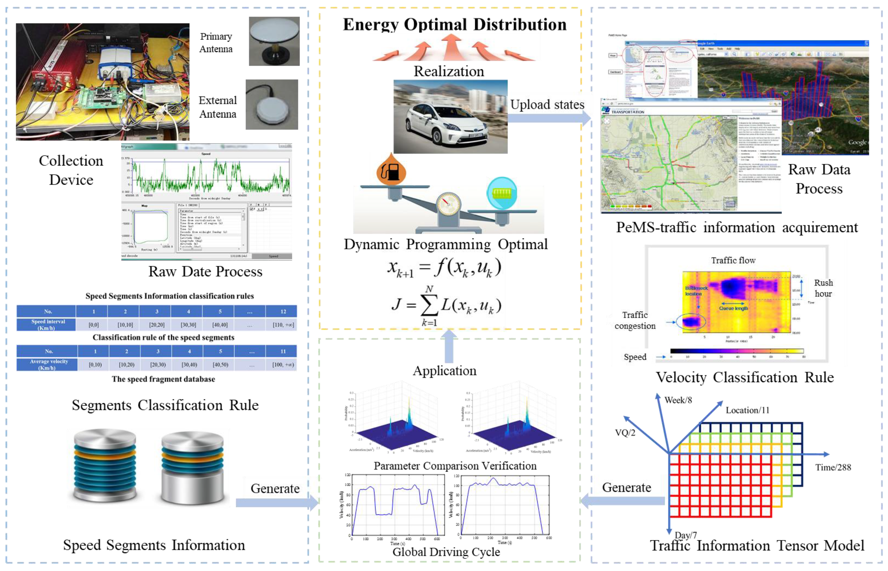
2. Local Database Construction Method

2.1. Velocity Segments Database Construction

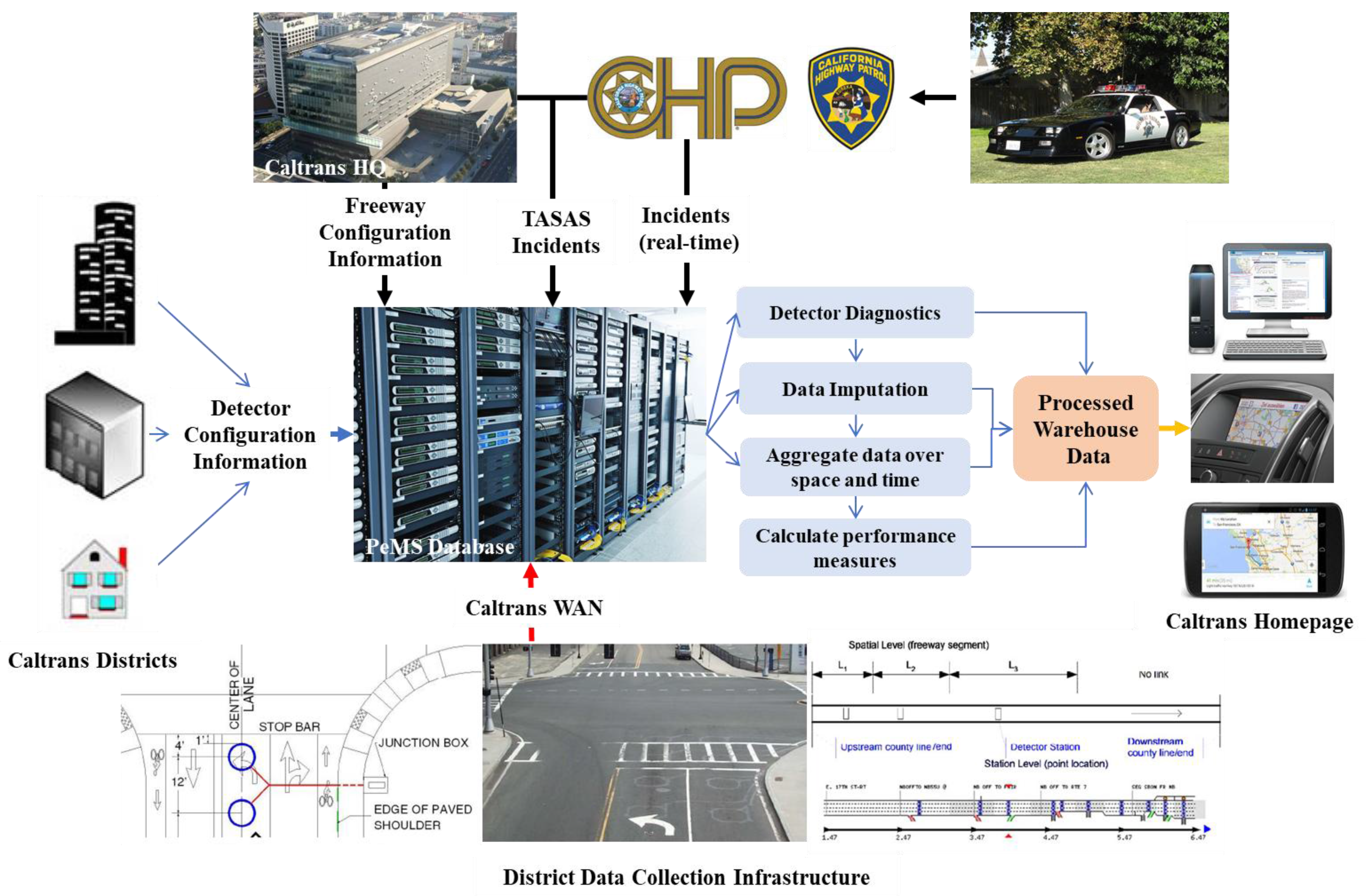
2.1.1. Driving Cycle Data Acquisition

The vehicle driving cycle is influenced by many factor, such as the road grade (main road, freeway, number of road lanes); traffic intensity (vehicle average velocity, vehicle volume, road saturation); cross density (cross type and quantity within the section); time influence (early rush, late rush, working day), and so on.

The driving cycles are downloaded from the California Department of Transportation performance measure system (PeMS), which were collected by floating cars on urban roads, suburban roads and freeways in California [17,18,19]. The acquisition period is approximately from 7:00 to approximately 22:00, and lasted for eight weeks.

2.1.2. Driving Cycle Data Classification Rule

The traditional kinematic sequences usually use the velocity segments from when the vehicle starts to its next idle for one velocity fragment, and this method is mainly used in the construction of urban public transport driving cycles or urban rush hour vehicles driving cycle construction [20,21]. However, with circumstance such as suburbs or urban highways with a high velocity and low idle time, they cannot well reflect true road driving conditions. In this paper, the working conditions are collected on different types of roads, so the kinematic parameters of the working conditions are obviously different. It is especially obvious in the morning and evening rush hours. According to the traditional kinematic segmentation method, this will lead to long kinematic fragments, moreover, there is only one kinematic segment in a construct driving cycle. To construct a more general-velocity database, the principle of this paper is as follows. Firstly, the collected data are divided into different velocity interval kinematic segments according to the ladder velocity interval. The velocity segments classification rule can be seen in

Table 1. Classification rule of the velocity segments.

Classification Items	1	2	…	12
Velocity interval (km/h)	[0,0]	[10,10]	…	[110,110]

.

The velocity fragment database is constructed based on the average velocity of the kinematic sequences. Every velocity fragment set is classified by the average velocity range. The detail classification rule is shown in

Table 2. The velocity fragment database.

Classification Items	1	2	…	11
Average velocity (km/h)	[0,10)	[10,20)	…	[100,+∞)

.

To prevent a long kinematic fragment leading the formation driving cycle that only has one velocity segment, the maximum velocity segment length based on the empirical method is set to 200 s.

2.2. Real-Time Traffic Information Model Construction

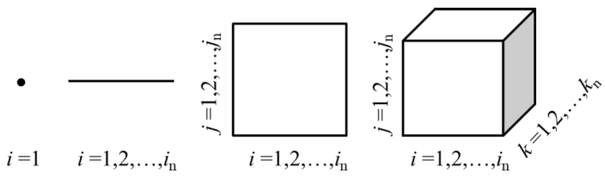
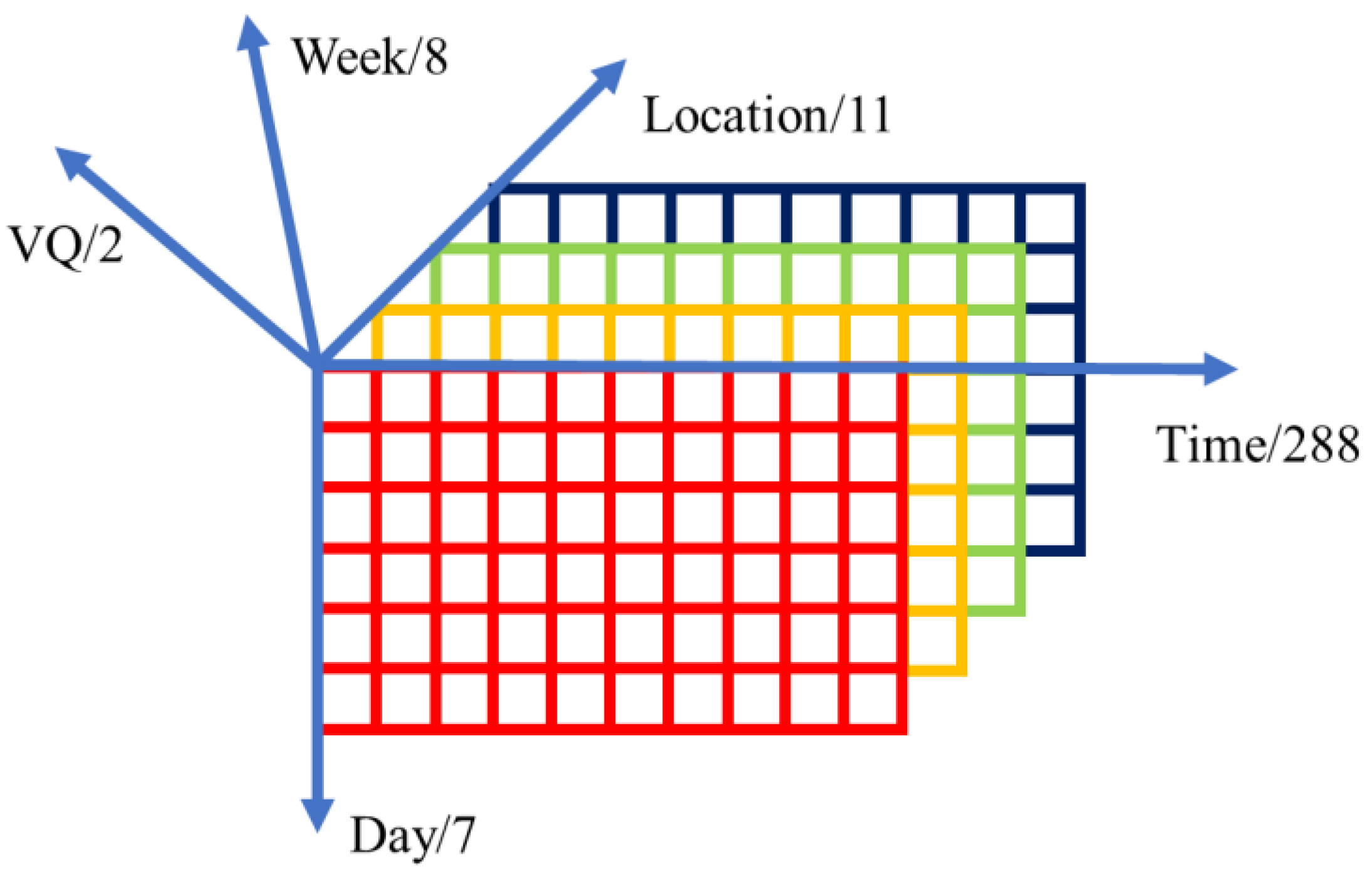
2.2.1. Tensor Introduction

Tensor, also known as N-mode matrix, is a high-order generalization of scalar, vector and matrix [22,23,24,25]. The scalar can be regarded as a zero-order tensor, the vector can be regarded as a first-order tensor and the matrix can be regarded as a second-order tensor. $A\in R^{I_1{I}_2\dots I_n}$ can be regarded as a N-order tensor. The elements of A can be demonstrated as with 1 ≤ i_n ≤ I_n. When the I_n = 3, the third-order tensor can be shown as a cube. The zero-, first-, second- and third-order tensor is shown in Figure 1 below.

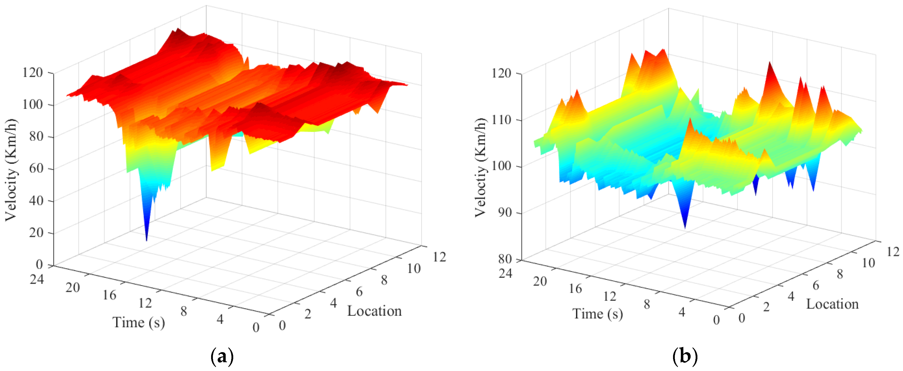
2.2.2. Traffic Information Analysis

This paper constructs a traffic information tensor model from the perspective of multi-mode information mining. The freeway data in the model are from the data of the open source traffic information database of PeMS as well. The brief structure of the system is shown in Figure 2. The vehicle detector station (VDS), which uses traffic loop pre-placement under the road to collect traffic information, including vehicle velocity and number, and so forth. This information will be provided as reference to evaluates road traffic condition. All the traffic information uploads in the database every five minutes, which will record 288 traffic information in 24 h. The raw data through further processed by the system traffic information process can be accessed conveniently by selecting the required traffic information from the Caltrans homepage.

In this paper, the traffic information is collected from the California section of the freeway for eight weeks, which contains 11 traffic loops, a total length of about 13 km. According to the multi-mode characteristic of traffic information, it can construct the five-dimensional tensor form of Time (288) × Day (7) × Week (8) × Location (11) × VQ (2) (Figure 3). Where Day has 288 dimensions, indicating the number of times the traffic is detected in the day; Day has seven dimensions, representing the week’s data, Week has eight dimensions, representing the tensor model for eight weeks’ mode; location has 11 dimensions, indicating that there are 11 vehicle detection base stations; VQ has two dimensions, indicating that the tensor model has two modes, namely, the average road velocity and road traffic volume. Based on the tensor model, the real-time traffic data is analyzed by using the multi-linear analysis. The relationship between the real-time traffic information and the real-time vehicle velocity can be clearly revealed by the tensor model.

The reason we chose the tensor structure to store data is the convenience of the transform process. For example, based on the tensor model of Tensor_VQ, Tensor_VQ (:, 1, 2, 1, 1) means the velocity of the first day at the second week at position 1 in time domain form database, and Tensor_VQ (204, 1, 2, :, 1) means the road velocity distribution in the first day at the second week at 17:00 in the spatial domain. We can change the number to realize different kinds of data from the time domain to the spatial domain that we needed. Due to the convenience of the tensor model calculation, this paper uses the tensor model to store traffic information; the data structure can quickly construct the required data sets and reveals the relationship between the traffic information and vehicle velocity.

In probability theory, covariance is a parameter measuring the intensity and direction relationship of two stochastic numbers. It is widely used in linear relation between stochastic numbers. The calculation formula is given below.

$$\mathrm{cov}(x,y)=E[(x-E(x))(y-E(y))]$$

(1)

where E(x) means the expected value of x, known, as the mean of x.

Correlation coefficient is a number quantifying the correlation and dependence between two or more stochastic numbers. The formula is

$${\rho }_{x,y}=\frac{\mathrm{cov}(x,y)}{{\sigma }_x{\sigma }_y}=\frac{E(xy)-E(x)E(y)}{\sqrt{E(x^2-E^2(x))}\sqrt{E(y^2-E^2(y))}}$$

(2)

where cov(x, y) means the covariance between x, and y. σ_x is the standard deviation.

Correlation coefficient matrix is constructed by the correlation coefficient among the elements. The construction law is shown below.

$${\theta }_{i,j}=\frac{\mathrm{cov}(x_i,x_j)}{{\sigma }_{x_i}{\sigma }_{x_j}}=\frac{E(x_i{x}_j)-E(x_i)E(x_j)}{\sqrt{E(x_i^2-E^2(x_i))}\sqrt{E(x_j^2-E^2(x_j))}}$$

(3)

$$CM=\left[\begin{array}{ccc}{\theta }_{1,1}& \dots & {\theta }_{1,n}\\ \dots & \dots & \dots \\ {\theta }_{n,1}& \dots & {\theta }_{n,n}\end{array}\right]$$

(4)

The correlation coefficient matrix of the two most basic properties: correlation coefficient matrix is symmetric, and its angular elements are 1.

If we considering the whole traffic information as one part, then the correlation coefficient can be calculated by

$$C=\frac{{\displaystyle {\sum }_{n\ge i\ge j\ge 1}{\theta }_{i,j}}}{n(n-1)/2}$$

(5)

Table 3. Road average velocity correlation coefficient matrix.

Time	8:00	8:05	8:10	8:15	8:20	8:25	8:30	8:35	8:40
8:00	1.000	0.996	0.990	0.986	0.964	0.949	0.818	0.700	0.793
8:05	0.996	1.000	0.998	0.997	0.982	0.975	0.867	0.765	0.846
8:10	0.990	0.998	1.000	1.000	0.991	0.982	0.877	0.786	0.860
8:15	0.986	0.997	1.000	1.000	0.994	0.986	0.887	0.802	0.871
8:20	0.964	0.982	0.991	0.994	1.000	0.991	0.908	0.846	0.898
8:25	0.949	0.975	0.982	0.986	0.991	1.000	0.952	0.889	0.941
8:30	0.818	0.867	0.877	0.887	0.908	0.952	1.000	0.974	0.998
8:35	0.700	0.765	0.786	0.802	0.846	0.889	0.974	1.000	0.985
8:40	0.793	0.846	0.860	0.871	0.898	0.941	0.998	0.985	1.000

is the road average velocity correlation coefficient matrix from 8:00 to 8:40. The correlation coefficient distribute between 0.7 and 1.0, which means that the road average velocity has a strong correlation. Using average velocity to generate driving cycle based on high correlation can improve the accuracy of driving cycle parameters.

The Figure 4a below shows the average velocity of the road at different times on Monday, x-axis represents 288 velocity data which were collected in 24 h; y-axis shows the 11 VDS locations in the test road; z-axis represents the average velocity in the test road. Red color means high velocity and blue color means low velocity. The average daily velocity of the test road obviously changes: the average velocity of the test road is clearly declining at the early rush (about 7:00 to 9:00) and the late rush (17:00 to 19:00), for which the road average velocity is lower, approximately 30 km/h–60 km/h.

The Figure 4b shows the road average velocity on Sunday. Compared with the average road velocity on Monday (Figure 4a), the road velocity does not change obviously on Sunday. It has no obvious morning and evening rush, full-day velocity is relatively stable compared with workdays. The velocity is mainly distributed in the 100 km/h to 110 km/h range. And the average velocity is the same as the non-rush hour velocity on Monday. Overall, the road average velocity has a strong relationship with time, and the y-axis shows the whole road velocity changing slightly at non-rush hour; therefore, it is reasonable to generate the driving cycle considering the road average velocity according to the time.

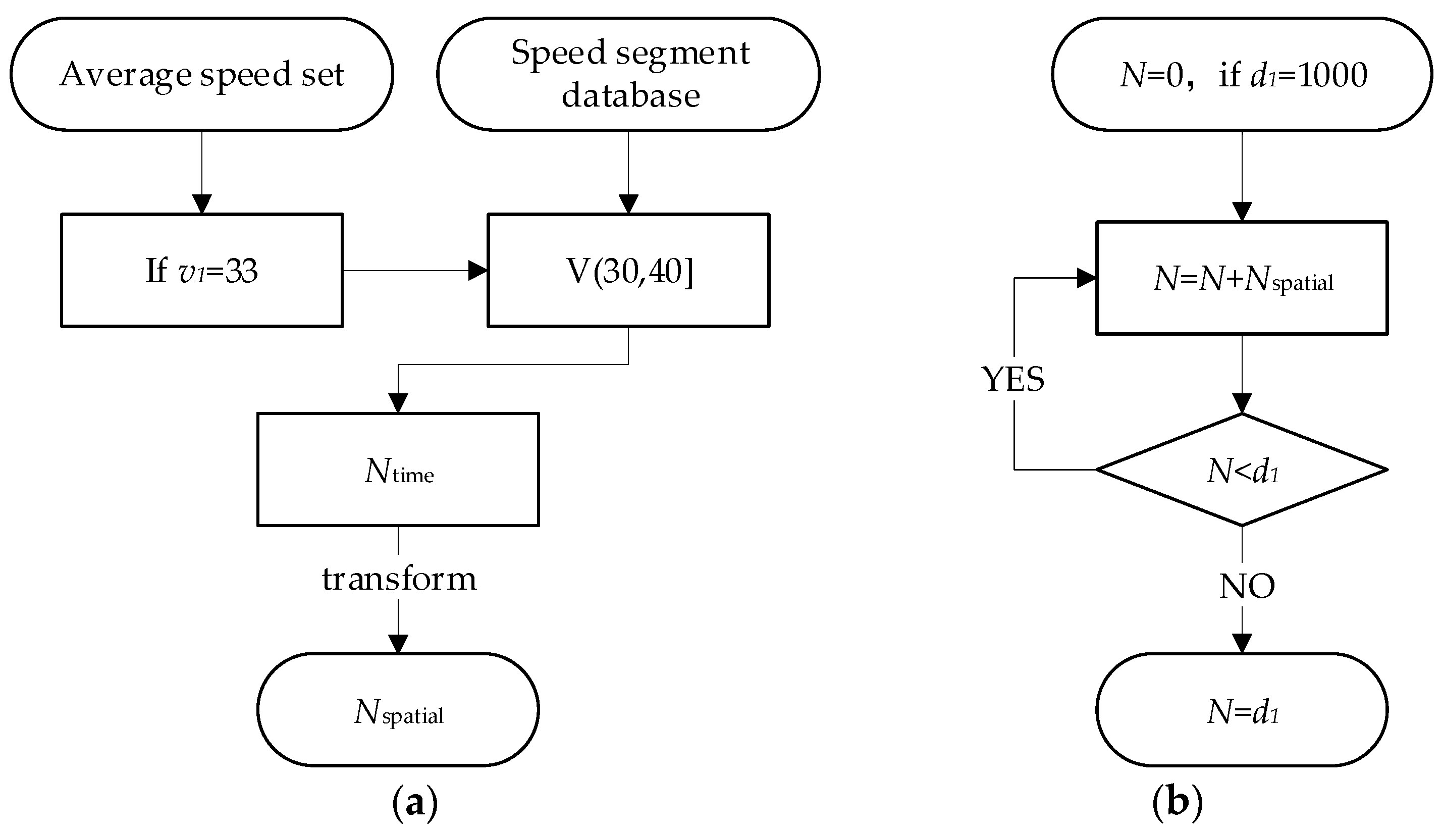
3. Freeway Driving Cycle Construction

According to the 11 VDSs on the experiment road, the freeway was divided into 11 sections, recorded as d_i (i = 1, 2, …, 11). Each road section has its own average velocity in traffic information tensor model, which is the main driving cycle construction reference. According to the current time of the road section, the average velocity is randomly chosen from the velocity segments database to combine the real-time driving cycle. The specific real-time driving cycle is achieved as follows: supposing that the vehicle start at t, then the control unit calculated with each road section velocity form the current position to the destination at this time based on the traffic information tensor model. Then the selected velocity segments form the corresponding database to sequentially construct the first road section driving cycle. The construction will stop when the construction freeway driving cycle (CFDC) extends beyond current road section length. The next road section will construct until all the road section driving cycles are completely constructed. At the start and end phases of the vehicle, we selected the velocity segment database average acceleration synthesis rate from 0 to the segment average velocity of the fragment, and vice versa. Because of the sudden change in the velocity of the connection between the different velocity segments during the process synthesis, this is different from the actual driving velocity. Therefore, it is necessary to eliminate the error caused by the velocity changing suddenly by filtering. The filtered driving cycle can be used as a driving cycle at time t. Then, 300 s later, we updated the current position road section average velocity, repeating the method above to generate the current time driving cycle.

Figure 5a is an example showing how we constructed the minimum segment constructing driving cycle segment based on real-time. Note that N_spatial is the minimum segment in this method. When we get the average velocity set form PeMS at the t moment, assuming the average velocity on this road segments is 33 km/h in this example, then we stochastically choose the velocity segment in the corresponding database. Due to this segment are stored in the time domain (velocity changing with time), we should transform it to the spatial domain (distance changing with time).

Figure 5b depicts the principle of generate a driving cycle between VDS. When we get the N_sptial, we use it to structure the road segments’ driving cycle, assuming the road segment is 1000 m and N equal to sum of N + N_spatial. Then, judging whether the distance of N is beyond the d₁, if N is less than d₁, we repeat the cycle until N is more than the d₁ length. We then scratch the length equal to d₁ from the beginning.

4. Global Optimal Energy Management Control Strategy

4.1. Economic Driving System

Figure 6 depicts the EDS methodology which contains four procedures to construct a closed-loop frame structure, including the local database construction process, PeMS data download process, FDC generation process and energy optimal control management process. Before the driver leaves the start position, the driver inputs the destination in the car navigation system, the navigation system will calculate the optimal route from the local position to the destination, and download the real-time traffic information stored in tensor model from the PeMS database through the internet; then, this information and velocity segments information, which download in advance in nearly all kinds of driving conditions, are provided as a database; the FDC is generated based on the classification rule and speed segments information, as well as real-time traffic information tensor model; finally, these FDCs are applied as the inputs of optimal energy management control strategy in PHEV with using a DP algorithm to calculate the optimal control sequence including state of charge (SOC) consumption curve to program the energy distribution. To achieve a closed loop, the vehicle real-time corresponding traffic information is collected by the vehicle detector system (VDS) on the freeway and uploaded to the PeMS in real time.

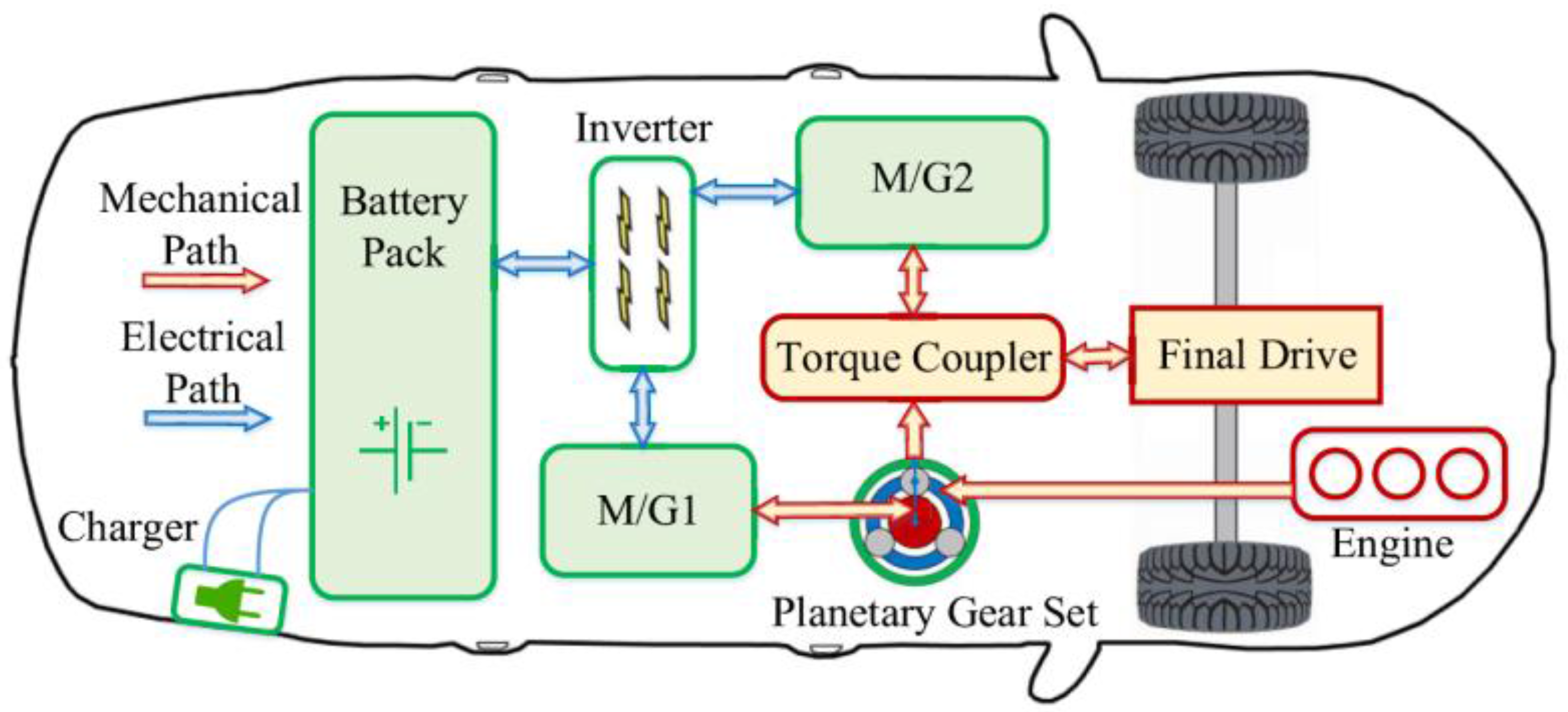
4.2. PHEV Transection Structure and Parameters

There are three kinds of power transfer structure in PHEV: series type; parallel type, and; mixed type. In this paper, the model vehicle adopts dynamic separation transmission with mixed type (Figure 7) [26,27,28], and the specific vehicle parameters are shown in the

Table 4. Plug-in electric hybrid vehicle (PHEV) parameters in this paper.

Component	Parameters	Quantity
Engine	Displacement	1.8 L
	Max Power	57 kw
	Max Torque	110 Nm
Motor/Generator	M/G1 Max power	30 kW
	M/G2 Max power	35 kW
Battery	C-LiFePO4	6.5 Ah
Transmission	E-CVT
Vehicle	Curb weight	1400 kg
	Frontal area	2.23 m2
	Drag coefficient	0.26
	Drive wheel radius	0.287 m

. M/G1 M/G2 are motor which has generator function to realize braking energy recovery.

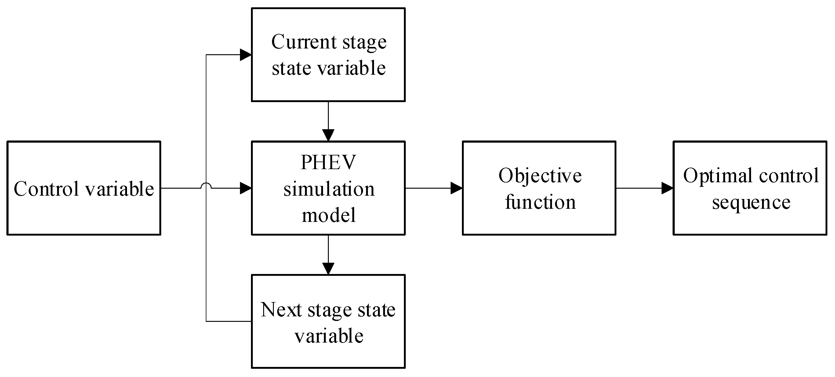
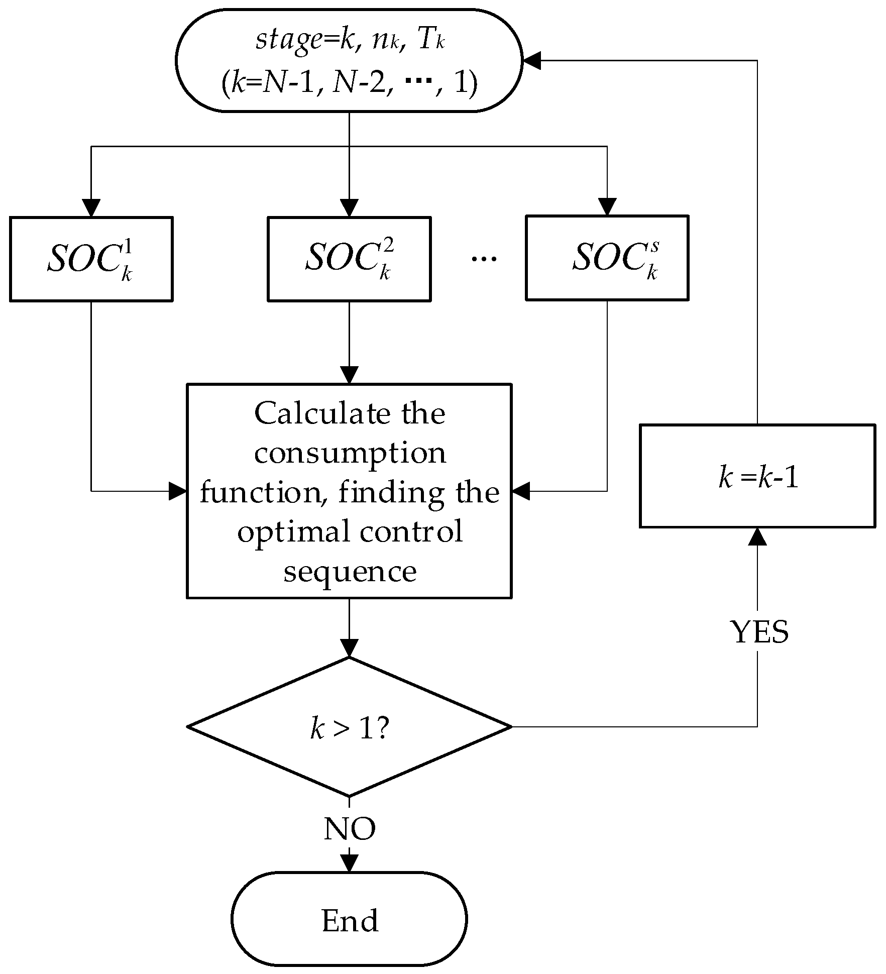
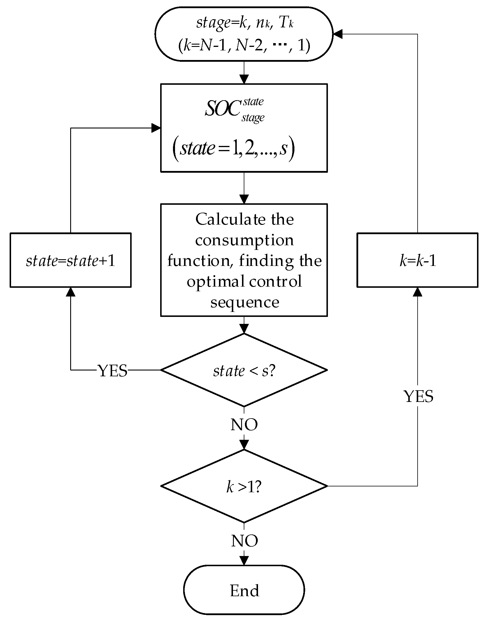
4.3. Optiamal Problem Construction

DP algorithm is a method which decomposes a problem to some sub-problems, solving each of those sub-problems just one time, and storing the results [29,30]. Optimal substructure and overlapping sub-problems are the prerequisites for using DP. When the same sub-problem occurs again, the CPU does not need to repeat calculate it twice, only needing to look up the database which was stored before. Therefore, DP algorithm saves calculation time by using a storage database, and this idea in the academic field is called “memoization” (not to be confused with memorization).

Optimal substructure and overlapping sub-problems are the prerequisites for using DP. If an optimization problem solution can be solved by the combination of problems to its sub-problems. These optimal substructures are called recursion in the field of computing. For a classic problem of calculating the shortest path from the start to the end, if the recursive algorithm dealing with the problem computation method is the same as the sub-problems rather than computing a new sub-problem, these problems are called overlapping sub-problems. The recursive formulation for generating the Fibonacci series is a classic example.

As the global energy management based on DP can achieve optimal energy control compared to other energy management strategies, it is usually used to calibrate the effectiveness of other control strategies such as charge deleting, charge sustaining control strategy (CDCS), which uses electricity at first then maintains SOC to protect battery health (Figure 8).

The application of this method requires the vehicle driving cycle in advance, but the global driving cycle construction method is seldom studied, which leads to the fact that this method has not been applied in real vehicles. From the method based on traffic information, the tensor model and velocity segment database we discussed above, this article realizes the online reconfiguration of the driving cycle, and provides data support for DP of online vehicle applications.

The methodology of DP using in PHEV energy management control strategy contains several parts, including state variable, control variable, simulation model and objective function. The working structure is shown below. In the current stage, the control variables act on the system model, which leads to the transfer of the state of the system and the transfer of the state cost to the objective function. At the next stage, the state of the system after the transfer will be the original state of the stage, thus cycle, and output the optimal set of control variables (Figure 9).

In the discrete time domain, PHEV is used as a system which can be described by the equation

$$x_{k+1}=f(x_k,u_k)$$

(6)

where x_k+1 is the system state at k + 1 moment, x_k and u_k are the system state and corresponding control variable, respectively.

The PHEV, which carries larger batteries, hopes to partially substitute fossil fuels with grid power. Therefore, the global optimal energy management problem of PHEV becomes the problem of minimizing the cost function of hybrid system control sequences. The cost function is shown in the formula below.

$$J={\displaystyle \sum _{k=1}^{N}L(x_k,u_k)}$$

(7)

where J is the total fuel consumption in the optimization process; N is the number of phases after time domain discretization depending on the sampling step of the working condition; L(x_k, u_k) is the instantaneous fuel consumption at k moment.

The constraint conditions of the cost function are shown below.

$$\begin{array}{c}{T}_{eng\_min}\le T_{eng}\le T_{eng\_max};{\omega }_{eng\_min}\le {\omega }_{eng}\le {\omega }_{eng\_max};T_{MG1\_min}\le T_{MG1}\le T_{MG1\_max};\\ {\omega }_{MG1\_min}\le {\omega }_{MG1}\le {\omega }_{MG1\_max};T_{MG2\_min}\le T_{MG2}\le T_{MG2\_max};{\omega }_{MG2\_min}\le {\omega }_{MG2}\le {\omega }_{MG2\_max};\\ SO{C}_{batt\_min}\le SOC\le SO{C}_{batt\_max};I_{batt\_min}\le I_{batt}\le I_{batt\_max};P_{batt\_min}\le P_{batt}\le P_{batt\_max};\end{array}$$

(8)

The computation time affects the real-time application in the vehicle, therefore, it is one of the essential points to consider in DP energy control management strategy. Calculation time mainly depends on the computation velocity of the processor and computation amounts. With the rapid development of autopilot technology, efficient CPU is widely applied in automobile control systems. The control CPU used in this paper is i5-6500, with a main frequency of 3.2 GHz, and a maximum of 3.6 GHz.

For the computation amounts, the question is how to select the appropriate calculation set in relation to the amount of calculation time. According to the preview studies, we select an optimal calculation interval, which is show below.

The state calculation is 0.001, which will get the ideal calculation time based on experiment and previous research group studies [31].

According to the driving distance, we selected a reasonable SOC interval for the DP to compute. This interval selected rule is based on historical data and empirical formula. For instance, the vehicle will be driving for approximately 10 km, assuming the SOC is 0.8 at this moment, the control unit will set this driving process consuming 0.1 SOC according to historical data and the empirical formula, then the DP algorithm will calculate the optimal driving control sequence with the SOC interval from 0.8 to 0.6.

To save the DP calculation time, the parallel solve method (Figure 10) is applied instead of the traditional series solve method (Figure 11). The stage various calculation process is process at the same time. Therefore, the calculation time will be nearly 1/N compared with series solve method.

5. Results and Discussion

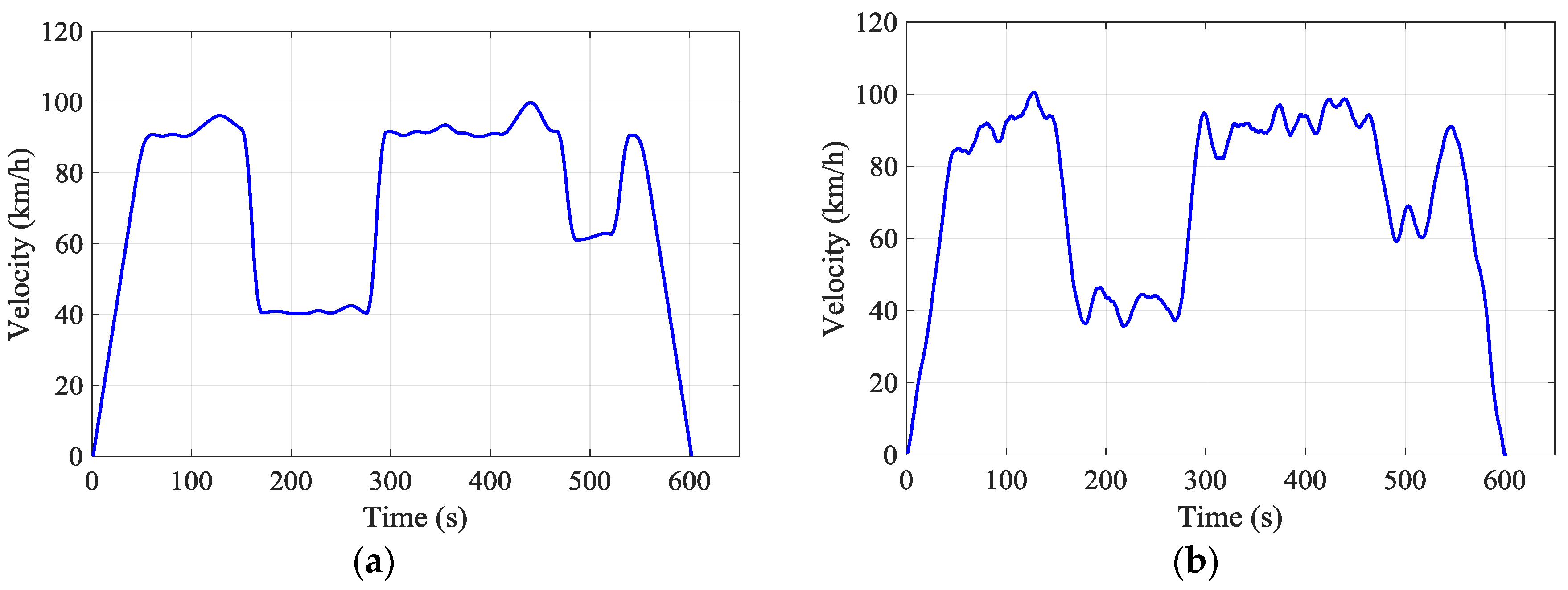
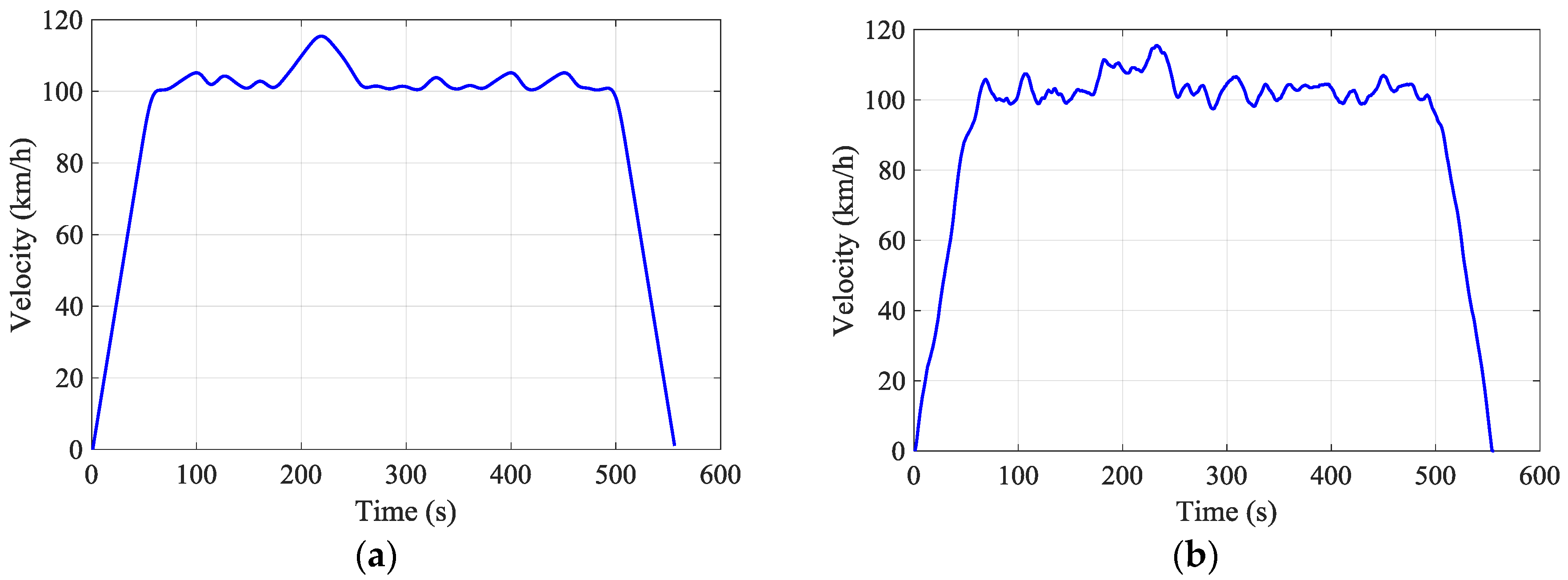
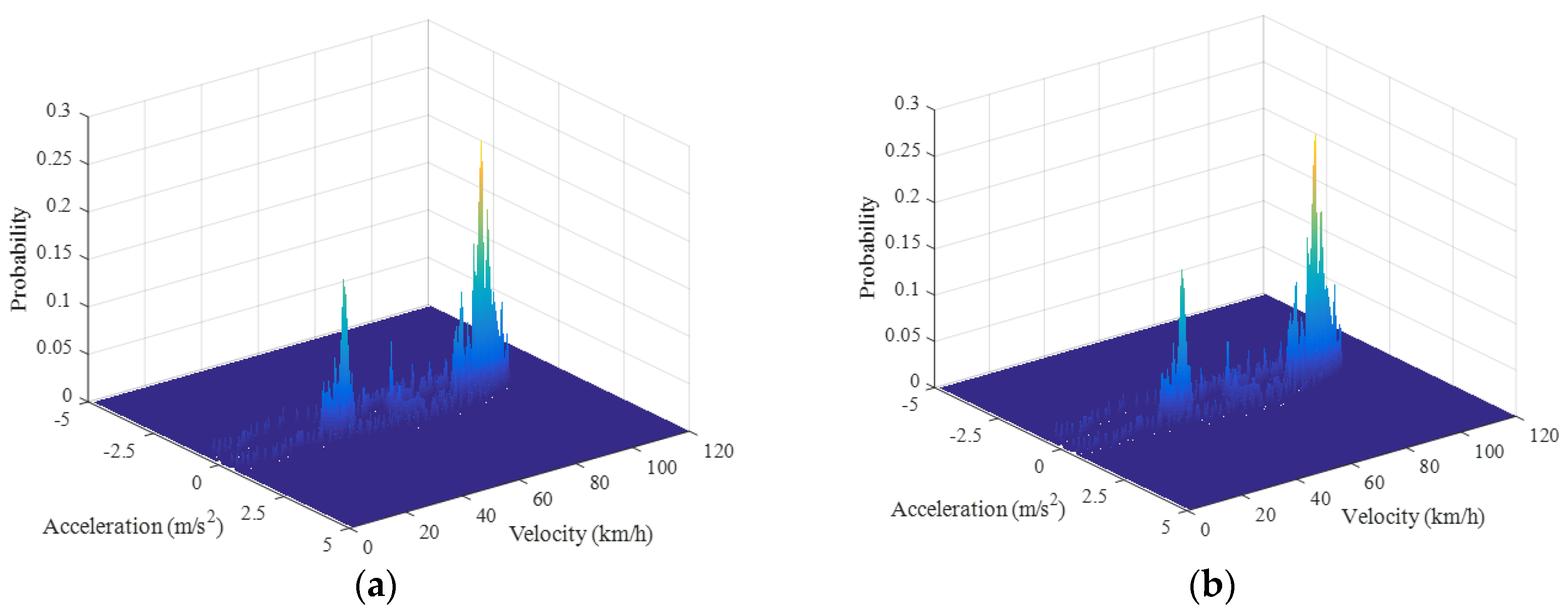
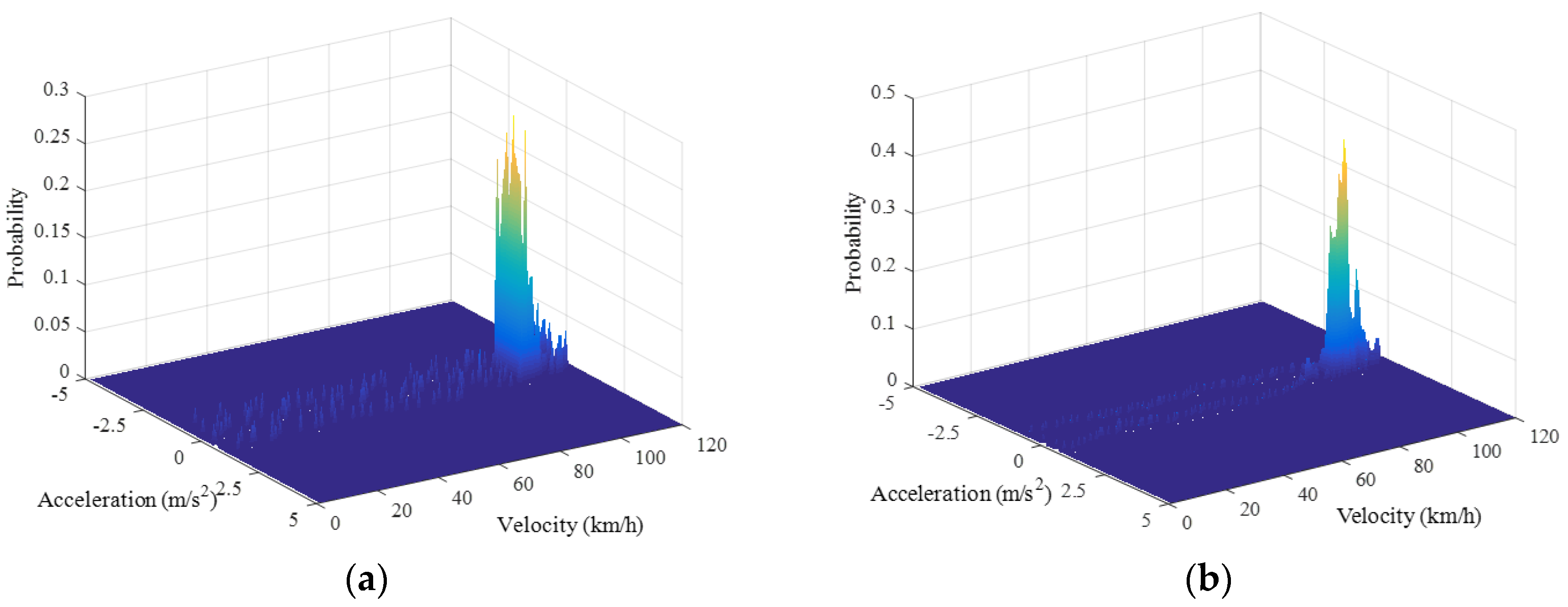
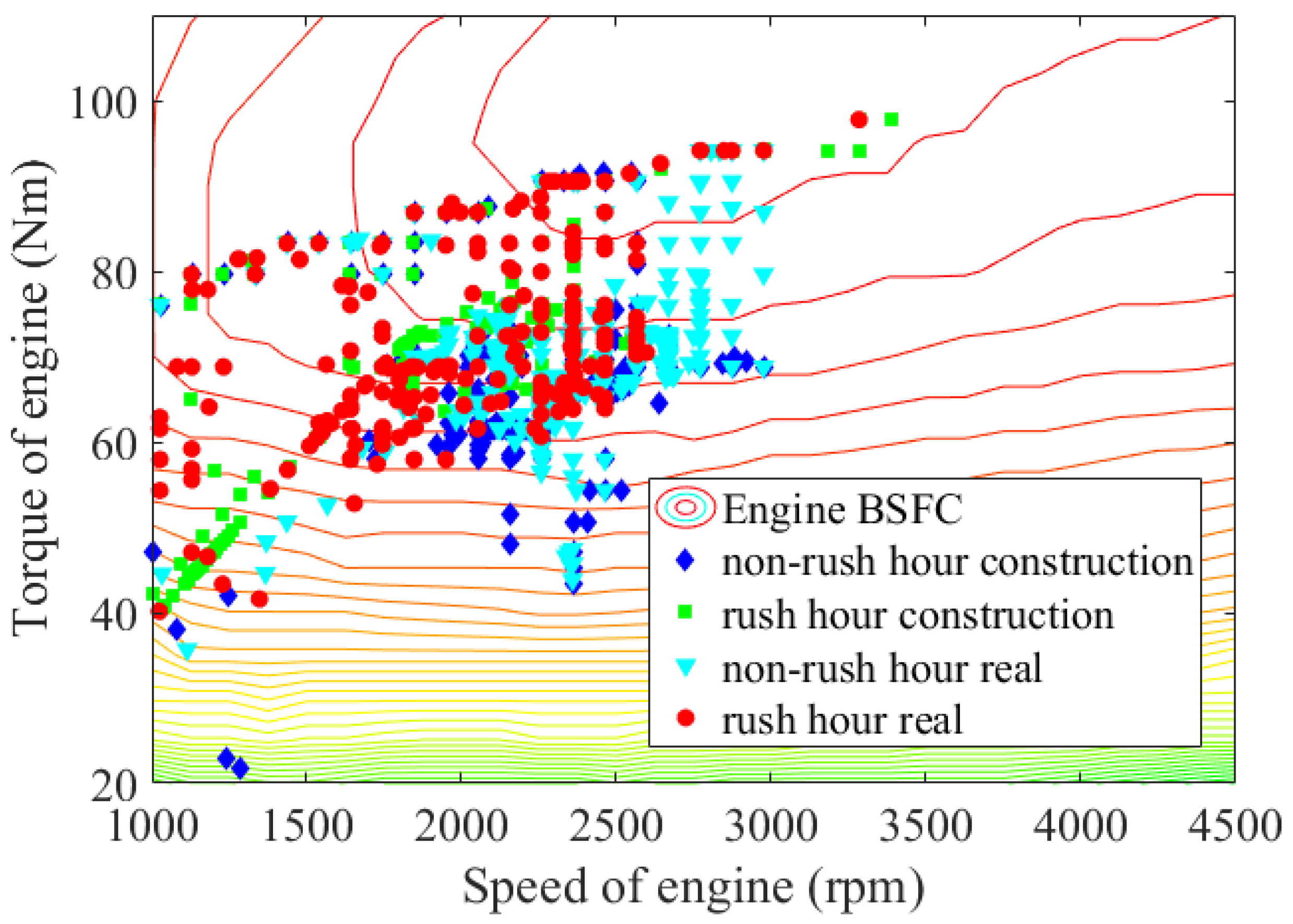
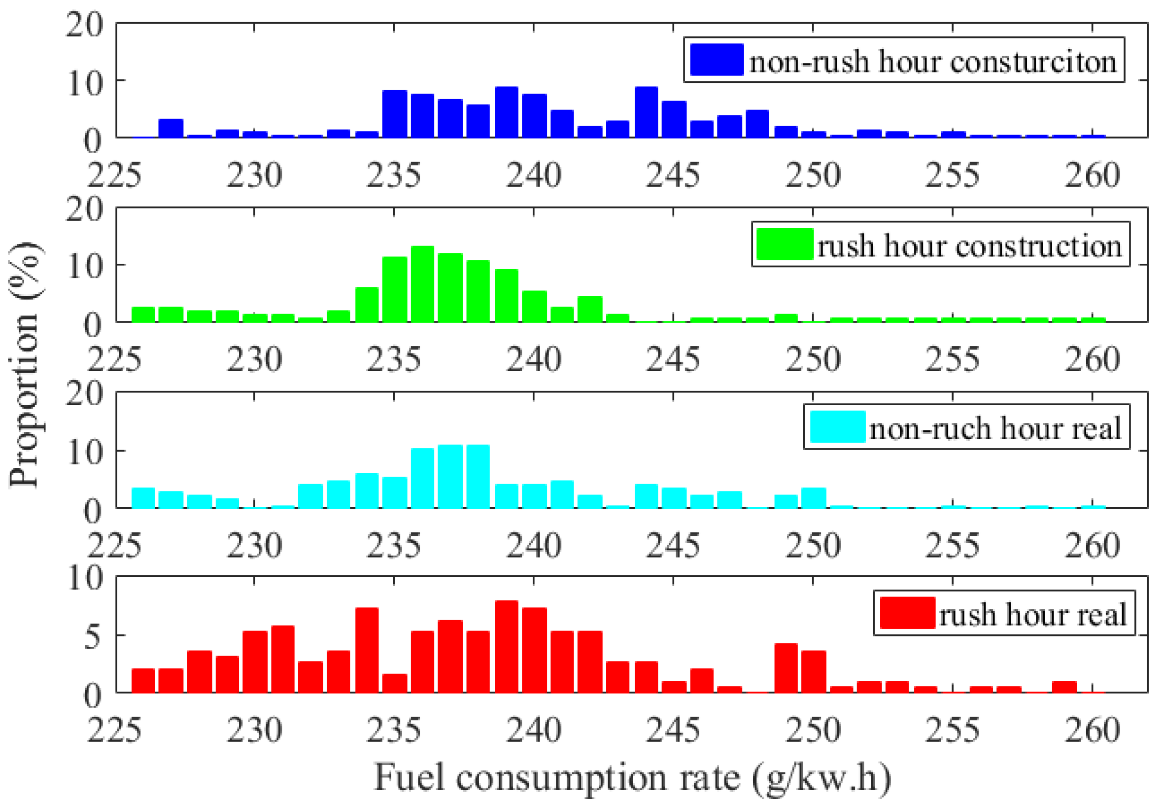
5.1. Analysis of the Freeway Driving Cycles

It is reasonable to generate the overall situation at morning or evening rush hour due to the fact that the average velocity will obviously be reduced compared with other time. In this circumstance, the driving cycle has a typical parameter which has great influence on the diving construction process. The CFDC shows this method can indicate the RFDC when the road average changes due to the traffic congestion phenomenon. The CFDC and collection RFDC are shown in Figure 12a,b, respectively. The CFDC velocity changing tendency resembles the RFDC and this method responds efficiently when the average road velocity changes suddenly, such as at approximately 180 s to 280 s. The kinematic parameters of the various conditions are shown in

Table 5. Characteristic parameters at rush hour.

Items	CFDC	RFDC
Avg. velocity (km/h)	70.85	70.75
Max. velocity (km/h)	99.87	100.51
Max. acceleration (m/s2)	4.06	3.21
Max. deceleration (m/s2)	−4.05	−3.77
Acceleration time proportion	52.25%	49.58%
Deceleration time proportion	47.75%	50.08%

. By contrast, it can be concluded that the construction conditions can be a good response to the actual operating conditions.

The CFDC generated during the non-rush hour are compared with the RFDC in Figure 13a,b, respectively. The kinematic parameters are shown in the

Table 6. Characteristic parameters at non-rush hour.

Items	CFDC	RFDC
Avg. velocity (km/h)	92.57	92.81
Max. velocity (km/h)	115.39	115.51
Max. acceleration (m/s2)	2.8	3.05
Max. deceleration (m/s2)	−2.5	−2.77
Acceleration time proportion	52.79%	50.63%
Deceleration time proportion	47.21%	49.19%

. The parameters are similar to the real vehicle acquisition parameters, and the generated future conditions can well approximate the real vehicle conditions.

The following Figure 14 is the velocity-acceleration probability distribution (VAPD) map describing the acquaintance between the CFDC and the RFDC at rush hour. The velocity and acceleration distributions are similar at rush hours, and parameter probability are concentrated in similar acceleration and velocity intervals.

Figure 15 shows the VAPD at non-rush hour section, the kinematic parameters probability distribution is similar between CFDC and RFDC, and all the driving cycle velocity are concentrated at around 100 km/h. This means that the CFDC well reflects the RFDC. All these results proved that this method can properly construct the global real-time driving cycle.

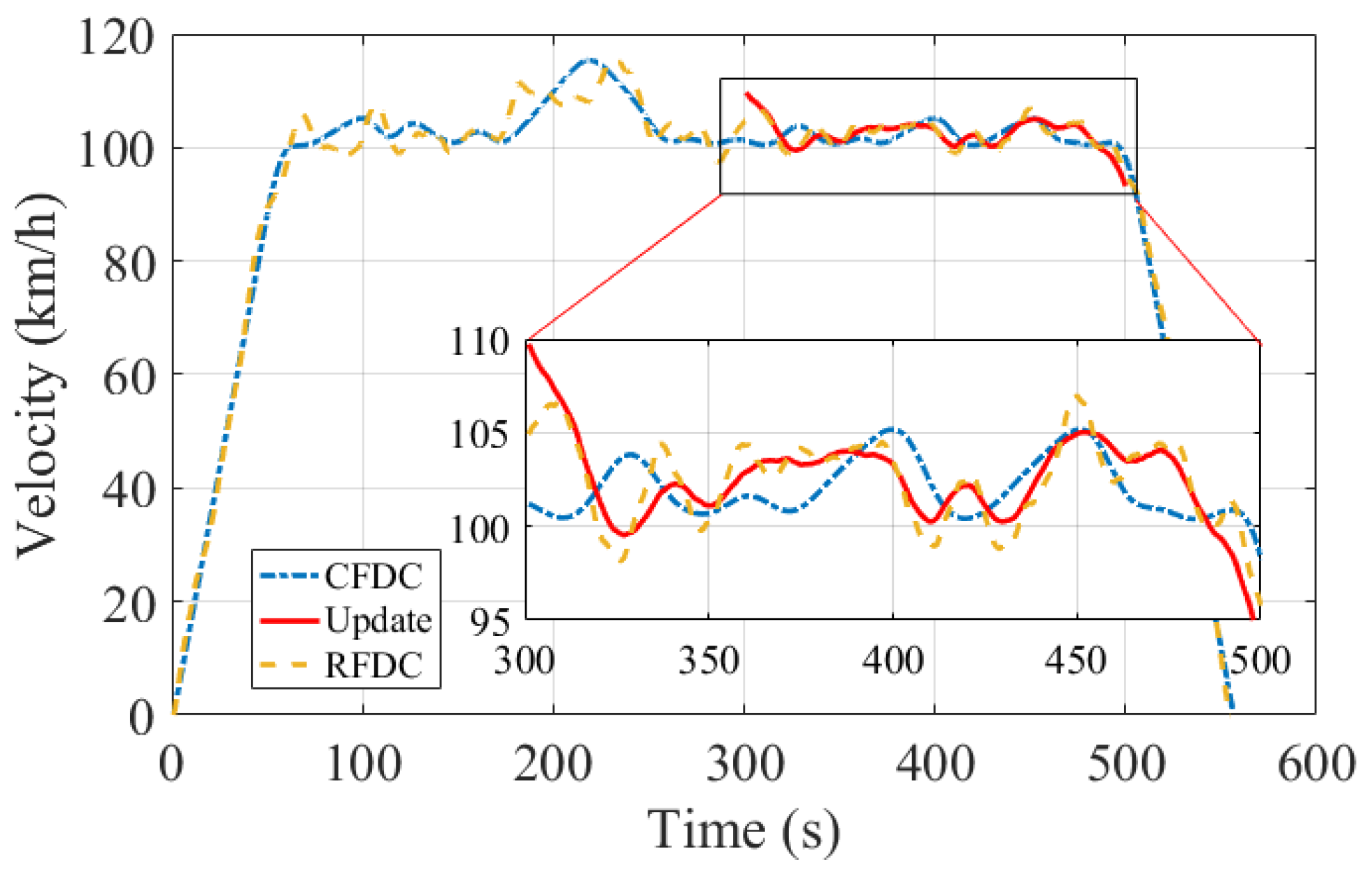
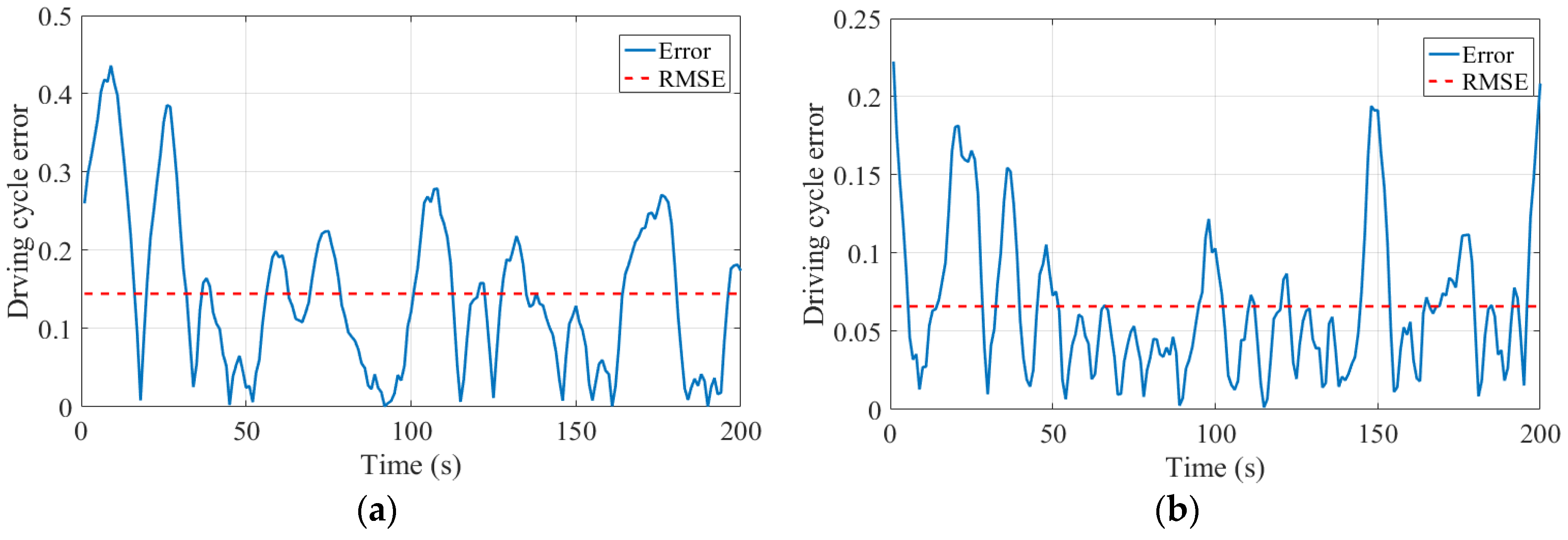
5.2. Update Construction Freeway Driving Cycle Error Analysis

When it has completed a set of global FDC, the vehicle can refer to it to realize optimal rational distribution of oil and electricity. After 300 s, the global FDC will be reconstructed from the current position to the end point. The starting velocity of the new generator starts from the current average speed. Due to the update traffic information compared with original traffic information, the new global FDC at the current moment can be more accurately (Figure 16) compared with previous global FDC. The global FDC (root mean squared error) RMSE after 300 s has obviously declined from approximately 0.141 to 0.065 (Figure 17a,b), which quite well reflects the actual road conditions.

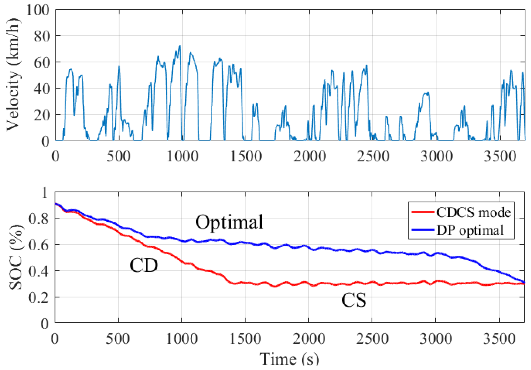
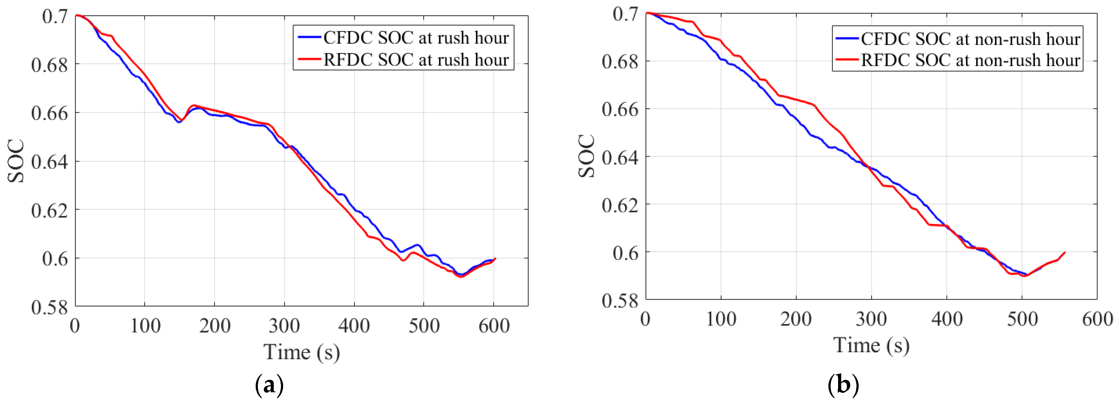
5.3. Global Optimal Energy Management

We applied the global FDC which was mentioned above in the simulation PHEV model. The engine working points distribution map (Figure 18) shows that DP energy control strategy making the engine work, in a majority of conditions, in the high efficiency area. The corresponding fuel cost proportion of each CFDCs’ fuel is specifically shown in Figure 19.

Based on the driving distance, the SOC reduces 0.07 from 0.7 to 0.63 at rush hour and reduces 0.1 from 0.7 to 0.6 at non-rush hour (Figure 20). The SOC consumption curves have similar features in the same circumstances. Due to the vehicle velocity at rush hour being reduced at a rate of approximately 150 s to 300 s, the SOC consumption rate has a reduced tendency in the same time interval, and this proves that the vehicle model is reasonable, which reflects the optimal SOC curve with a different driving cycle.

DP control strategy and rule-based control strategy with the same driving cycle are simulated with the PHEV model (

Table 7. Energy consumption comparison at rush hour.

Item	DP		Rule Based
Driving cycle	RFDC	CFDC	RFDC	CFDC
Fuel cost (L/100 km)	4.15	4.29	4.63	4.75
SOC cost	0.1	0.1	0.1	0.1
Ratio of fuel cost	100.00%	103.37%	111.57%	114.46%

and

Table 8. Energy consumption comparison at non-rush hour.

Item	DP		Rule Based
Driving cycle	RFDC	CFDC	RFDC	CFDC
Fuel cost (L/100 km)	3.34	3.51	3.82	3.95
SOC cost	0.07	0.07	0.07	0.07
Ratio of fuel cost	100.00%	105.09%	114.37%	118.26%

).

Specifically speaking, compared with rule-based control strategy [32,33], the DP control strategy ratio of fuel cost is much lower: a reduction of almost 13.17% in fuel cost compared with ruled-based control strategy in the same CFDC at non-rush hour. This result proved control strategy based on DP has the best performance In rule-based control strategy, the fuel efficiency at rush hour is much more efficient than at non-rush hour (fuel cost 11.57% higher than DP compared with fuel cost 14.37% higher than DP). Moreover, in DP control strategy, the CFDC fuel consumption error (3.37%) at rush hour is less than at non-rush hour error (5.09%).

Overall, all of the CFDCs’ fuel consumption are higher than RFDCs. At nearly the same driving distance, non-rush hour fuel consumption is less than rush hour fuel consumption (3.51 (L/100 km) at non-rush hour, 4.29 (L/km) at rush hour); steady state is one of the reasons in this circumstance, which is like cruise control function in some vehicles and has great energy economy characteristics.

6. Conclusions

A novel FDC construction method and global optimal energy management is proposed in this paper to improve the fuel economy of PHEVs.

• The history and real-time traffic information tensor model are constructed and the correlation between real-time traffic information from the perspective of time domain and spatial domain are deeply explored.
• The variation law of road velocity and the change rule of working day and weekend are clarified. The validity of the FDC construction method is proved by comparing the CFDC and RFDC.
• The FDC uses real-time traffic information, which is applied for the first time in the driving cycle construction method, and the parameter between CFDC and RFDC are in the reasonable error horizon.
• The driving cycles are applied in PHEVs to achieve real-time optimal control strategy based on the DP algorithm. There are fuel economy rates of up to 14.37% compared with rule-based control strategy.

In the future, tensor filling algorithms with missing traffic information and road section completion will be further explored. Moreover, hardware-in-loop will be introduced to further verify the fuel economy as well.

In the future, we will explore how to construct the driving cycle with incomplete traffic information, which we preliminarily plan to solve by using tensor filling algorithm and explore a method to increase road sections to enhance FDC construction accuracy. Moreover, urban driving cycle construction method will be explored in the future as well.

References

1. Armas, O.; García-Contreras, R.; Ramos, Á. Impact of alternative fuels on performance and pollutant emissions of a light duty engine tested under the new European driving cycle. Appl. Energy 2013, 107, 183–190. [Google Scholar] [CrossRef]
2. Fontaras, G.; Franco, V.; Dilara, P.; Martini, G.; Manfredi, U. Development and review of Euro 5 passenger car emission factors based on experimental results over various driving cycles. Sci. Total Environ. 2014, 469, 1034–1042. [Google Scholar] [CrossRef] [PubMed]
3. Damiano, A.; Musio, C.; Marongiu, I. Experimental validation of a dynamic energy model of a battery electric vehicle. In Proceedings of the International Conference on Renewable Energy Research and Applications, Palermo, Italy, 22–25 November 2015; pp. 803–808. [Google Scholar]
4. Zhang, S.; Xiong, R. Adaptive energy management of a plug-in hybrid electric vehicle based on driving pattern recognition and dynamic programming. Appl. Energy 2015, 155, 68–78. [Google Scholar] [CrossRef]
5. Galgamuwa, U.; Perera, L.; Bandara, S. Developing a General Methodology for Driving Cycle Construction: Comparison of Various Established Driving Cycles in the World to Propose a General Approach. J. Transp. Technol. 2015, 5, 191–203. [Google Scholar] [CrossRef]
6. Li, M.; Zhu, X.; Zhang, J. A Study on the Construction of Driving Cycle for Typical Cities in China. Automot. Eng. 2005, 27, 557–560. [Google Scholar]
7. Jian, P. Study on the Construction of Urban Mixed Road Driving Condition; Hefei University of Technology: Hefei, China, 2011. [Google Scholar]
8. Jiang, P.; Shi, Q.; Chen, W.; Huang, Z. A Research on the Construction of City Road Driving Cycle Based on Wavelet Analysis. Automot. Eng. 2011, 33, 70–73. [Google Scholar]
9. Hung, W.T.; Tong, H.Y.; Lee, C.P.; Ha, K.; Pao, L.Y. Development of a practical driving cycle construction methodology: A case study in Hong Kong. Transp. Res. Part D Transp. Environ. 2007, 12, 115–128. [Google Scholar] [CrossRef]
10. Chen, Z.; Xiong, R.; Wang, C.; Cao, J. An on-line predictive energy management strategy for plug-in hybrid electric vehicles to counter the uncertain prediction of the driving cycle. Appl. Energy 2017, 185, 1663–1672. [Google Scholar] [CrossRef]
11. Li, L.; Yang, C.; Zhang, Y.; Zhang, L.; Song, J. Correctional DP-Based Energy Management Strategy of Plug-In Hybrid Electric Bus for City-Bus Route. IEEE Trans. Veh. Technol. 2015, 64, 2792–2803. [Google Scholar] [CrossRef]
12. Banvait, H.; Anwar, S.; Chen, Y. A rule-based energy management strategy for plug-in hybrid electric vehicle (PHEV). In Proceedings of the American Control Conference, St. Louis, MO, USA, 10–12 June 2009; pp. 3938–3943. [Google Scholar]
13. Padmarajan, B.; Mcgordon, A.; Jennings, P. Blended rule based energy management for PHEV: System Structure and Strategy. IEEE Trans. Veh. Technol. 2016, 66, 8757–8762. [Google Scholar] [CrossRef]
14. Zhang, J.; Shen, T. Real-Time Fuel Economy Optimization with Nonlinear MPC for PHEVs. IEEE Trans. Control Syst. Technol. 2016, 24, 2167–2175. [Google Scholar] [CrossRef]
15. Pahasa, J.; Ngamroo, I. PHEVs Bidirectional Charging/Discharging and SoC Control for Microgrid Frequency Stabilization Using Multiple MPC. IEEE Trans. Smart Grid 2015, 6, 526–533. [Google Scholar] [CrossRef]
16. Son, H.; Kim, H. Development of Near Optimal Rule-Based Control for Plug-In Hybrid Electric Vehicles Taking into Account Drivetrain Component Losses. Energies 2016, 9, 420. [Google Scholar] [CrossRef]
17. Chen, C. Freeway Performance Measurement System (PeMS); University of California, Berkeley: Berkeley, CA, USA, 1 July 2003. [Google Scholar]
18. Varaiya, P.P. The Freeway Performance Measurement System (PeMS), PeMS 9.0: Final Report; Path Research Report; University of California, Berkeley: Berkeley, CA, USA, 30 November 2008. [Google Scholar]
19. Jia, Z.; Chen, C.; Coifman, B.; Varaiya, P. The PeMS algorithms for accurate, real-time estimates of g-factors and speeds from single-loop detectors. In Proceedings of the 2001 IEEE Intelligent Transportation Systems, Oakland, CA, USA, 25–29 August 2001; pp. 536–541. [Google Scholar]
20. Tong, H.Y.; Hung, W.T.; Cheung, C.S. Development of a driving cycle for Hong Kong. Atmos. Environ. 1999, 33, 2323–2335. [Google Scholar] [CrossRef]
21. Shi, Q.; Zheng, Y.; Jiang, P. A Research on Driving Cycle of City Roads Based on Microtrips. Automot. Eng. 2011, 33, 256–261. (In Chinese) [Google Scholar]
22. Kolda, T.G.; Bader, B.W. Tensor Decompositions and Applications. Siam Rev. 2009, 51, 455–500. [Google Scholar] [CrossRef]
23. Ali, M.; Foroosh, H. Character recognition in natural scene images using rank-1 tensor decomposition. In Proceedings of the IEEE International Conference on Image Processing, Phoenix, AZ, USA, 25–28 September 2016; pp. 2891–2895. [Google Scholar]
24. Sidiropoulos, N.D.; Lathauwer, L.D.; Fu, X.; Huang, K.; Papalexakis, E.E.; Faloutsos, C. Tensor Decomposition for Signal Processing and Machine Learning. IEEE Trans. Signal Process. 2017, 65, 3551–3582. [Google Scholar] [CrossRef]
25. Huang, K.; Sidiropoulos, N.D.; Liavas, A.P. A Flexible and Efficient Algorithmic Framework for Constrained Matrix and Tensor Factorization; IEEE Press: Piscatway, NJ, USA, 2016. [Google Scholar]
26. Zhou, Y.; Han, C.; Wang, X.; Yu, T. Research on power train source matching for single-axle PHEV. In Proceedings of the 2008 IEEE Vehicle Power and Propulsion Conference (VPPC’08), Harbin, China, 3–5 September 2008; pp. 1–4. [Google Scholar]
27. Pourabdollah, M.; Murgovski, N.; Grauers, A.; Egardt, B. Optimal Sizing of a Parallel PHEV Powertrain. IEEE Trans. Veh. Technol. 2013, 62, 2469–2480. [Google Scholar] [CrossRef]
28. Domingues, G.; Reinap, A.; Alaküla, M. Design and cost optimization of electrified automotive powertrain. In Proceedings of the International Conference on Electrical Systems for Aircraft, Railway, Ship Propulsion and Road Vehicles & International Transportation Electrification Conference, Toulouse, France, 2–4 November 2016; pp. 1–6. [Google Scholar]
29. Howard, R.A. Dynamic Programming and Markov Processes; The Technology Press of the Massachusetts Institute of Technology and John Wiley & Sons, Inc.: Providence, RI, USA, April 1961. [Google Scholar]
30. Bellman, R. Dynamic Programming. Science 1966, 153, 34–37. [Google Scholar] [CrossRef] [PubMed]
31. Wang, X. Optimization Study on Powertrain Matching and System Control for Plug-In Hybrid Electric Urban Bus; Beijing Institute of Technology: Beijing, China, 2015. [Google Scholar]
32. Cai, Y.; Ouyang, M.; Yang, F. Energy management and design optimization for a series-parallel PHEV city bus. Int. J. Automot. Technol. 2017, 18, 473–487. [Google Scholar] [CrossRef]
33. Huang, Y.J.; Yin, C.L.; Zhang, J.W. Design of an energy management strategy for parallel hybrid electric vehicles using a logic threshold and instantaneous optimization method. Int. J. Automot. Technol. 2009, 10, 513–521. [Google Scholar] [CrossRef]
Figure 1. Zero-, first-, second- and third-order tensor.
Energies 10 01796 g001
Figure 2. Brief structure of the performance measure system (PeMS).
Energies 10 01796 g002
Figure 3. Traffic information tensor model.
Energies 10 01796 g003
Figure 4. (a) Velocity on Monday; (b) Velocity on Sunday. Red color means high velocity and blue color means low velocity.
Energies 10 01796 g004
Figure 5. (a) Nspatial flow chart; (b) Segment flow chart.
Energies 10 01796 g005
Figure 6. Economy driving system.
Energies 10 01796 g006
Figure 7. Power transmission structure.
Energies 10 01796 g007
Figure 8. State of charge (SOC) comparison between charge deleting charge sustaining (CDCS) and dynamic programming (DP).
Energies 10 01796 g008
Figure 9. Schematic diagram of DP structure and operation process.
Energies 10 01796 g009
Figure 10. Parallel solver flow chart.
Energies 10 01796 g010
Figure 11. Series solver flow chart.
Energies 10 01796 g011
Figure 12. (a) Construction freeway driving cycle (CFDC) at rush hour; (b) real freeway driving cycle (RFDC) at rush hour.
Energies 10 01796 g012
Figure 13. (a) CFDC at non-rush hour; (b) RFDC at non-rush hour.
Energies 10 01796 g013
Figure 14. (a) CFDC velocity-acceleration probability distribution (VAPD) at rush hour; (b) RFDC VAPD at rush hour.
Energies 10 01796 g014
Figure 15. (a) CFDC VAPD at non-rush hour; (b) RFDC VAPD at non-rush hour.
Energies 10 01796 g015
Figure 16. Updated global freeway driving cycle.
Energies 10 01796 g016
Figure 17. (a) CFDC error and root mean squared error (RMES); (b) Updated CFDC error and root mean squared error (RMSE).
Energies 10 01796 g017
Figure 18. Working point distribution of engine in different driving cycles.
Energies 10 01796 g018
Figure 19. Fuel cost proportion of different control strategies.
Energies 10 01796 g019
Figure 20. (a) SOC comparison at rush hour; (b) SOC comparison at non-rush hour.
Energies 10 01796 g020