1. Introduction
Financial institutions are facing increasing challenges in mitigating various kinds of risks. In his “taxonomy of risks”,
Christoffersen (
2011) defines risks as market volatility, liquidity, operational, credit and business risks. Due to uncertainties, financial risk evaluation (FRE) is increasingly playing a pivotal role in ensuring organizations maximize their profitability by minimizing losses due to a failure to mitigate risks.
Noor and Abdalla (
2014) argue that there is a direct negative impact on profitability in proportion to unmitigated risks. Hence, the primary approach of FRE is to identify risks in advance to allow for an appropriate course of action before any investments or decisions can be made. As financial risks evolve over time due to factors such as economic fluctuations, market conditions and other factors beyond control, the evaluation process requires constant update to keep up with market conditions.
Credit risk analysis undertaken in recent years mostly involves financial risk prediction. For example, loan default analysis, which often comes in the form of binary classification problems, has become an integral part of FRE. As financial institutions today are dealing with millions of customers, the traditional human approach for loan approval processes are no longer feasible. Moreover, with the advent of computing power today coupled with the advancement of machine learning algorithms and the availability of large volume of information, the world has entered the renaissance of computational modeling with non-parametric classification methods and machine learning for loan default prediction becoming widely adopted. It is worth noting that machine learning classification achieves an accuracy that directly increases the bottom line whilst providing instantaneous approval decision through real-time decisions.
The use of advanced computing power and machine learning algorithms to predict whether a loan is performing or non-performing (NPL) is increasingly essential for the longevity of any lending institute. As the pool of consumers enlarges with proportional increases in spending, the ability to provide early warnings by accurately predicting the probability of defaulting a loan has become even more crucial. Deploying advanced machine learning algorithms to identify patterns from large features in high-volume data has become a mandatory process by banks to minimize the NPLs, and thus to increase their profitability and consumers’ confidence.
In this study, we aim our attention at loan default detection as an element of credit risk analysis through models built in k-nearest neighbour, naïve-bayes, decision tree, logistic regression, and random forest. The intention is to answer the following questions:
Is there a significant performance difference between the five machine learning algorithms piping through Scikit-learn data transformation steps?
Can the steps be repeated with the same level of consistency using different data sets but similar analytics pipelines with data transformation?
The study is arranged in the following way:
In
Section 2, we briefly cover the background of the rise of statistical methods used from the 60s to the 80s, primarily in the form of parametric approaches in predicting bankruptcy. This section also covers how modern predictive techniques were born in the 90s and beyond in conjunction with the availability of computing power, resulting in the advancements of this field.
In
Section 3, we conduct a case study to illustrate the use of the five machine learning algorithms to predict the loan default based on University of California at Irvine (UCI) data set. In this section, we present the analytics life-cycle methodology with emphasis on data pre-processing. It highlights the repeatability and validity of the methodology in conducting research.
In
Section 4, we construct various models and measure them using various tools, of which ROC-AUC is the main measurement. Other measurements are accuracy, precision, F1 score, etc. In this section, we draw comparisons between five classifiers and present the results neatly in various tables. We also present the out-of-sample prediction results to validate model accuracy.
2. Related Work
It is imperative for financial institutes to detect NPLs in advance and segregate them for further treatments. Unlike today, however, the ability to predict NPLs in the 60s was not commonplace due to the fact that data mining and predictive capabilities were in their embryonic state. During that era, financial analysis using a quantitative approach was in its nascent form. Mathematical models and statistical methods were basic compared to modern quantitative techniques. Apart from relying on studying a company’s financial statements, most financial risks analysis primarily relied on fundamental analysis which involves studying external factors such as market trends and economic indicators.
Beaver (
1966) laid a foundation of groundbreaking work in accounting, earning himself management using financial ratios. “Beaver’s Model” involved seminal univariate analysis to predict corporate failure.
Altman (
1968) devised the “Altman Z-Score” to predict the probability of whether a company will undergo bankruptcy. Beaver and Altman’s work pioneered approaches to financial risk analysis for the next decade.
Finance-related prediction in the 1970s hinged on Altman’s Z-Score, which had garnered popularity since the late 1960s. Although Altman’s work primarily involved predicting bankruptcy, academics and researchers adapted the underlying principles to perform prediction of risks to maintain financial health. The 1970s marked the emergence of modern risk management concepts with financial institutes becoming aware of the importance of identifying and managing various risk portfolios. The 1970s laid the groundwork for identifying and understanding financial risk prediction and management. This development was the beginning of the evolution of risk assessment methodologies and the adoption of risk management practices together. The regulatory frameworks aimed to enhance stability and resilience were set up by regulatory bodies.
Black and Scholes (
1973) developed the Black–Scholes–Merton (BSM) model in 1973 which aimed to calculate the theoretical price of European-style options. The model uses complex mathematical formulas and assumes standard normal distribution including logarithms, standard deviations (precursor to Z-Score) and cumulative distribution functions. The Black–Scholes–Merton model remains a foundation of today’s market risk assessment and serves as a fundamental tool for pricing options. Although specific research publications in the 1970s may not be common enough to be readily cited, many ideas, concepts and methodologies established during that timeframe set the stage for subsequent developments. Most notable is the gaining of traction of the quantitative approach to credit risk modeling and scoring. The rise of algorithms such as regression, discriminant analysis and logistic regression dominated the 1970s. The duo’s empirical results also demonstrated how efficient regulatory policy should be formulated from the regression outcomes.
Deakin (
1972), standing on the shoulders of Beaver and Altman, brought the analysis one notch higher using a more complex, albeit discriminatory, analysis to improve on the 20% error in misclassification of bankruptcy for the year prior. Deakin’s model of an early warning system assumed a random draw of samples and used various financial ratios and indicators including profitability ratios, efficiency ratios and liquidity ratios (amongst others) to distinguish between troubled and healthy firms.
Martin (
1977) leveraged the logit regression approach to predict the likelihood of banks experiencing financial distress.
The 1980s saw an increased focus on credit risk measurement within banking industries. Managing creditworthiness, credit exposures and the probabilities to default were key research topics by researchers and practitioners. Ohlson took interest of White and Turnbull’s unpublished work on systematically developed probabilistic estimates of failures.
Ohlson (
1980) used the maximum likelihood estimation methodology, which is a form of conditional logit model (logistic regression), to avoid the pitfall of well-known issues associated with multivariate discriminant analysis (MDA) deployed in previous studies. Ohlson’s model, primarily a parametric one (as most models were in that era), provided advantages in that no assumptions must be made to account for prior probabilities regarding bankruptcy and the distribution of predictors. Ohlson argued that Moody’s manual, as relied on by previous works, could be flawed due to the fact that numerous studies that derived financial ratios from the manual did not account for the timing of data availability and the complexity in reconstructing balance sheet information from the highly condensed report. In his concluding remark, Ohlson stated that the prediction power of any model depends upon when the financial information is assumed to be available.
West (
1985) combined the traditional parameter approach using a logit algorithm with factor analysis. West’s work was promising, as the empirical results show the combination of the two techniques closely matched the CAMEL rating system widely used by bank examiners in that era.
The 1990s and 2000s saw the birth of some exciting machine learning algorithms. Up until this point, most statistical methods used for credit assessment were related to the parametric approach. The parametric algorithms mandate that the assumptions of linearity, independence, or constant variance are met before meaningful analysis can be derived. The birth of Adaptive Boosting can be indebted to the work of
Freund and Schapire (
1997). The duo proposed that a strong classifier can be obtained by combining multiple weak classifiers iteratively.
Friedman (
2001) devised a method to improve the predictive accuracy by optimizing a loss function through iterative processes. Friedman’s gradient boosting machine (GBM) builds the trees sequentially, with each tree correcting by fitting the residuals of the previous trees. Friedman’s work was influential and subsequently gave rise to other boosting variations, including XGBoost by
Chen and Guestrin (
2016) and LightGBM by
Ke et al. (
2017).
Breiman and Cutler (
1993), however, proposed a way to construct multiple independent decision trees during training, with each tree deriving from a subset of training data and available features.
Breiman’s (
2001) random forest model ensures that each tree is trained on a bootstrap sample of data (random sample with replacement). The final prediction is made from aggregating the prediction from an ensemble of diverse decision trees. Vapnik and Chervonenkis’ early work dated as far back as the early 1960s in theory of pattern recognition, and statistical learning laid the groundwork for their support vector machine (SVM).
Vapnik’s (
1999) algorithm is known for the ability to classify both linear and non-linear data by finding the optimal hyperplane that best separates various classes whilst maximizing the margin between them.
Contemporary literature works in predicting financial risk has mushroomed over the past decade.
Peng et al. (
2011) suggest that a unique classification algorithm that could achieve the best accuracy given different measures under various circumstances does not exist. In their early attempts,
Desai et al. (
1996), and later
West (
2000), both proposed that the performance of generic models such as linear discriminant were not a better performer than customized models, except for a customized neural network. However, further studies by
Yobas et al. (
2000) using linear discriminant, neural network, genetic algorithms and decision tree concluded that the best performer was linear discriminant analysis. Due to the inconsistencies of previous studies,
Peng et al. (
2011) suggested multiple criteria decision making (MCDM), whereby a process to allow systematic ranking and selecting of an appropriate classifier or cluster of classifiers should be at the forefront of classification research. In the first ever academic study of Israeli mortgage,
Feldman and Gross (
2005) applied the simple yet powerful classification and regression tree (CART) to 3035 mortgage borrowers in Israel, including 33 features such as asset value, asset age, mortgage size, number of applicants, income, etc. The goal was to classify between potential defaulters and those unlikely to default. The distinct feature of CART that resulted in it being chosen over its primary competitors is its ability to manage missing data.
Khandani et al. (
2010) predicted the binary outcome that indicates whether an account is delinquent by 90 days by including the time dimension of 3-, 6- or 12-month windows. Using a proprietary dataset from a major bank, Khandani and others combined customer banking transactions (expenditures, savings and debt repayments), debt-to-income ratios and credit bureau data to improve the classification rates of credit card holders’ delinquencies and defaults. CART was chosen as the non-parametric approach due to its ability to manage the non-linearity nature of data and inherent explainability of the algorithm. Their work proved that the time series properties of the machine learning prediction commensurate with realized delinquency rates, with R
2 of 85%. He suggested assigning weight in training data as adaptive boosting to manage imbalanced class.
The rise of data gathering exercises made available hundreds or thousands of features compounded with imbalanced data, posing an issue for traditional approaches. The non-parametric approach burst onto the scene to manage the ever-increasing dimension, imbalanced data and the non-linear nature of models. The 2000s saw a rise of applying multi-layer neural networks and support vector machines (SVM) to financial prediction.
Atiya (
2001) proposed a non-parametric approach using a novel neural network model and was able to achieve accuracy of 3-year-ahead out-of-sample predictions between 81–85% accuracy.
Zhang et al. (
1999) suggested that artificial neural networks outperformed logistic regression.
Huang et al. (
2004) deployed backpropagation neural networks (BNN) and SVMs to achieve an accuracy of 80%.
Although the majority of datasets used for the studies are propriety in nature, there was little mention regarding the engagement of various data preparation techniques except from the recent study of the importance of data pre-processing effects on machine learning by
Zelaya (
2019) using the contemporary machine learning package such as Scikit-learn popularized by
Pedregosa et al. (
2011). The modern machine learning packages with full pipeline feature as shown by
Varoquaux et al. (
2015) are worth exploring. Equally omitted is the implementation of techniques such as SMOTE to manage imbalanced class, as proposed by
Fernández et al. (
2018), which is also worth further study.
In this study, we aim our attention at loan default detection as an element of credit risk analysis.
3. Case Study—Advanced Machine Learnings for Financial Risk Mitigation
3.1. Methodology—Computational Approach
In this study, the machine learning analytics cycle use Scikit-learn packages to implement an analytics pipeline that includes data collection, data pre-processing, model constructions and model performance comparisons. Matplotlib supplies graphing capability to allow for the visual analysis of data.
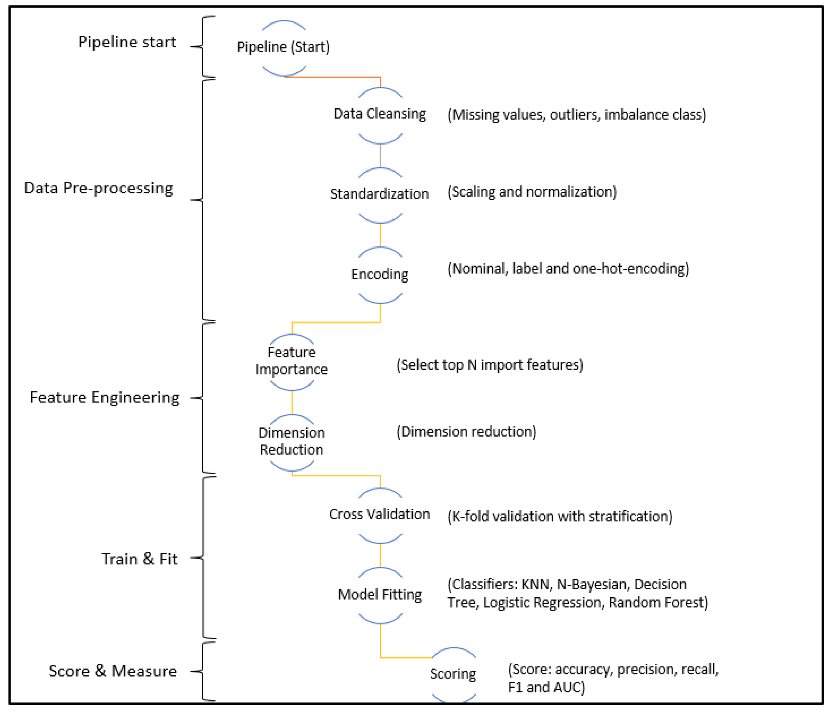
Scikit-learn allows for the full analytics pipeline to specifically unravel the underlying pattern in data sets, therefore resulting in the best fitting for various classifiers. The pipeline contains end-to-end processes that performs these tasks: (i) ingest the data sets and perform preliminary data analysis to identify missing values, outliers and imbalanced class—any missing values will be imputed and imbalanced data is identified; (ii) standardize data which includes scaling and normalization to ensure consistent model performance; (iii) encode categorical (nominal and ordinal) and one-hot-encode for predictors and label for target variable; (iv) select top N most influential predictors and reduce total dimension to the influential ones; (v) cross validate using k-fold stratified to ensure the ratio of imbalance remains intact and subsequently treated by SMOTE as suggested by
Chawla et al. (
2002); (vi) train and fit data using various distance- and tree-based classifiers; (vii) compare the final performance measurements and report the most effective hyper-parameters.
Figure 1 illustrates the machine learning analytics life cycle implemented as an end-to-end analytics pipeline using Scikit-learn’s pipeline capability.
The machine learning lifecycle is implemented as Scikit-learn’s pipeline, easing the foremost data pre-processing in missing value imputation with either the most frequent value (categorical features) or standard mean/median (numeric variable). The analytics pipeline detects outliers and imbalanced class, as well as manages the treatment of detection further down the pipeline right before the actual model fitting. Next is to apply data standardization, which includes transforming the data into a common scale using Z-Score, and normalize the data to a range between zero and one. The goal is to ensure data consistency across various classifiers which will result in comparisons at similar scales, thus improving model performance.
Subsequently, the analytics pipeline automatically detects the champion model (winner of the best classifier) and reports the top N predictors that are most influential to the model. The analytics pipeline finds the least influential predictors which subsequently truncated to reduce the dimension whilst not affecting the performance of the models. The analytics pipelines split the data into two sections with training and testing data segregated by a ratio of 80:20. The analytics pipeline implements k-fold with stratification to ensure that the imbalanced class stays intact. It also ensures a full data split throughout with little-to-no possibility of a data leak. Finally, it trains and fits the data through the five classifiers. At the end, it obtains the performance scores for final comparisons.
Apart from its stochastic nature, the research method is sound and repeatable, and researchers can refer to it for further studies with various data sets applied to different classifiers.
3.2. Data Collection
This study uses two credit card client data sets obtained from UCI repository.
The first set is the payment data set obtained from one major bank in Taiwan from 2005, donated by
Yeh and Lien (
2009) and
Yeh (
2016) to the UCI data repository. The data set holds 30,000 observations, of which 6636 are default payment (showed by variable id, x24 as 1) whilst healthy payment occupies the remaining 23,364 observations. The data set holds no duplicate and missing values. The Taiwan credit card payment data set shows a strong skew (healthy:default ratio) due to imbalanced class of 77.88% to 22.12%. The variable id, x24 is the target whilst it uses the remaining features (x1 to x23) as predictors (
Table 1).
This data set contains only numeric features. It is used as a control data set for the analytics pipeline due to its larger set of observations. It will be used to validate the analytics pipeline that includes data transformations.
The second set is a German credit card client data set obtained from UCI data repository,
Hofmann (
1994). It contains 1000 observations. The data set contains one target variable with an imbalanced class ratio of 70% to 30% (no:yes ratio). The data set is void of missing values and duplicates.
Table 2 shows the data set features, description and data types.
This data set contains both numerical and categorical data and is used to train and test various classifiers initially.
3.3. Visual Data Exploration
Either a classifier is parametric or non-parametric. Visual data exploration aids in understanding data structure and nature, which includes the data distributions, correlations, multi-collinearity and other patterns. Visual data exploration helps to identify anomalies and outliers in the data set that can skew analysis and model accuracy. In particular, the involvement of logistic regression and naïve-bayes necessitate a thorough analysis of data structure and patterns as these classifiers assume independence and linearity, amongst other things.
Table 3 reveals the correlation between numerical features.
As indicated in
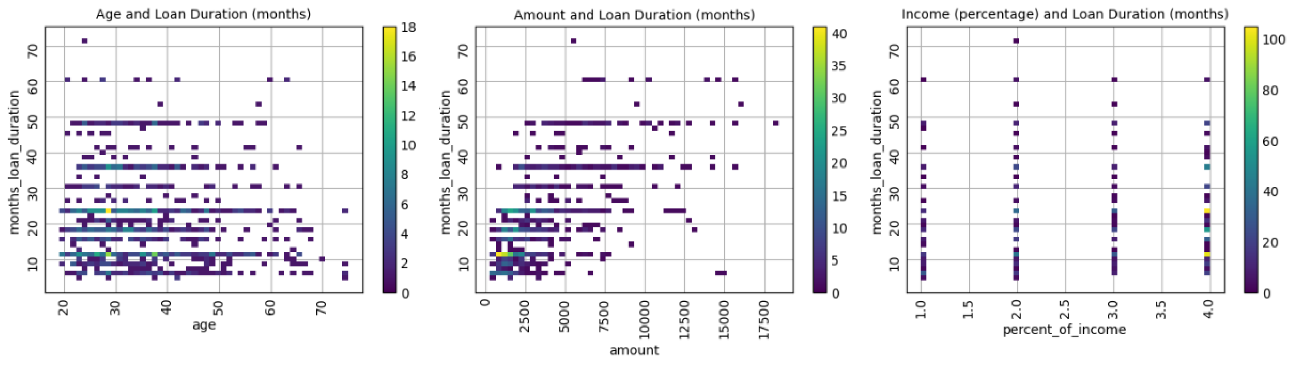
Table 3, the German credit data set has a low correlation between features. The highest correlation is 0.6250 between “months loan duration” and “amount”. It can be said that the correlation amongst other features is non-existent as indicated by scatterplots in
Figure 2. The only correlation of 0.6250 shows a positively trending linear relationship. However, “age” and “percent of income” do not show a visual pattern and therefore do not indicate a relationship with “months loan duration.”
Further investigation into multicollinearity of the German credit data set (
Table 4) shows that the variance inflation factor (VIF) values between predictors are reasonable and do not cause alarm.
The distribution of data can be considered partial-normal or normal (right skewed) for only three predictors, as seen in
Figure 3. The remaining numerical predictors are dichotomous in nature.
The final examination confirms that the German credit data set does not contain outliers or missing values.
3.4. Data Pre-Processing
The analytics pipelines correspond in a 1:1 ratio with the permutations of the test scenarios. The first analytics pipeline generates Permutation-1, the second generates Permutation-2, etc. The goal of having various permutations is to achieve the best model performance for the classifiers.
The analytics pipelines apply standardization, including scaling and normalization to all analytics pipelines in this study. For example, the k-nearest neighbour being a distance-based classifier requires that the features contribute more equally to distance calculation, therefore enhancing model performance. The pipelines ensure that there is no unintentional data leakage between the training and testing data sets.
After standardization, the analytics pipelines perform encoding (ordinal, one-hot and label encodings) for categorical features and class feature followed by imbalanced data treatment using SMOTE as investigated by
Alam et al. (
2020). Subsequently, the analytics pipelines reduce the dimensions of features to the system default and a preset number, respectively.
Prior to model training and fitting, the analytics pipelines implement a manual split of training/testing (80:20) data sets with stratification to ensure the imbalanced data ratio is intact. In search for the optimal hyper-parameters, the grid search function performs the 10-fold cross validations where data is split and internally evaluated for each fold.
3.5. Model Construction and Evaluation
During the model construction phase, the analytics pipeline includes the five classifiers (k-nearest neighbour, naïve-bayes, decision tree, logistic regression and random forest). The final prepared and split data, after being fully cleansed, standardized and encoded, has become a training source to fit the models. The only distance-based classifier used in this study is k-nearest neighbour. K-nearest neighbour is a simple, non-parametric classifier that is not subservient to the Gaussian distributions and is robust to outliers. The curse of dimension takes effect with k-nearest neighbour in that it poses two challenges: (i) it increases computational challenges when high dimensions and large data sets are involved and (ii) it degrades model accuracy when including irrelevant features.
The two tree-based methods are decision tree and random forest. Similar to k-nearest neighbour, decision tree is a tree-based classifier and can manage non-linearity and outliers well. Decision tree has an inherent ability to be unaffected by non-related features. However, the downside is that it tends to overfit. In this study, the analytics pipeline considers the tree-depth hyper-parameter to ensure that the decision tree classifier does not overfit. Random forest as an ensemble method inherits the strength from decision tree. Additionally, unlike decision tree, it aggregates the prediction of multiple decision trees and offsets the tendency to overfit.
Logistic regression and naïve-bayes are the only two parametric approaches used in this study. That said, they are susceptible to independence assumptions, non-linearity and outliers. In addition, imbalanced data affects naïve-bayes predictions. The analytics pipeline includes the data pre-processing to ensure the training is conducive to fit using the five classifiers, in particular, the parametric ones.
Table 5 illustrates the characteristics of the classifiers implemented in this study.
Whilst these dependency and tolerance level are common in the statistical and machine learning techniques, not all analyses require these assumptions to be met. Under certain conditions, there are methods to relax these dependencies and increase tolerance for the classifiers. Blatant ignorance of the requirements based on each classifier’s characteristic will result in poor and unreliable models.
As far as model measurement is concerned,
Han et al. (
2022) outlined the limitations of relying only on the rate of error as the default measurement as suggested by
Jain et al. (
2000) and
Nelson et al. (
2003). Since most of dataset one (Taiwan credit card client) is made up of non-risky value (77.88%), the error rate measurement is not appropriate as it is insensitive to the classification accuracy. The main measurement in this study is AUC despite the fact that
Lobo et al. (
2008) asserted that area under the receiver operating characteristic (ROC) curve, known as AUC, has its own limitations. Furthermore, the study includes error rate measurement which includes accuracy, precision, recall (sensitivity) and F1 score for the sake of completeness.
Table 2 shows the four error rate-related measurements in model evaluations:
Accuracy provides the proportion of correctly classified instances from the total instances.
Precision provides the ratio of true positive predictions versus the total number of positive predictions made.
Recall provides the proportion of actual positives correctly predicted by the model.
F1 provides a balance mean of precision and recall that deals with imbalanced class.
Table 6 depicts the performance metrics used throughout the model comparisons.
All the scores used in this study are based on prediction results.
4. Results
The results of the experiments are made up of performance metrics in tabular and graph formats as well as variables of importance in graph format. The results compare the performances based on the two distinct data sets with three permutations of analytics pipelines. Due to the stochastic nature of classifiers, the results differ slightly for each run. The red dotted line for ROC-AUC graphs represents a random guess for random guess.
The analytics pipelines produce three permutations in search of the best performing classifiers with their respective hyper-parameters.
Table 7,
Table 8 and
Table 9 and
Figure 4,
Figure 5 and
Figure 6 list the performance metrics for various permutations. All permutations include data cleansing and standardization:
Permutation-1—with or without SMOTE using the default hyper-parameters and scoring using full features (all predictors).
Permutation-2—with or without SMOTE using the best hyper-parameters and scoring using full features (all predictors).
Permutation-3—with or without SMOTE using the best hyper-parameters and scoring using reduced features (best performing predictors).
The tables and figures summarize the results:
Table 7 and
Figure 4—Permutation-1 by using German credit data set with the default hyper-parameters and full features.
Table 8,
Figure 5 and
Figure 7—Permutation-2 by using German credit data set with the best hyper-parameters and full features.
Table 9,
Figure 6 and
Figure 8—Permutation-3 by using German credit data set with the best hyper-parameters and reduced features.
Table 10,
Figure 9 and
Figure 10—Permutation-2 using Taiwan credit data set with the best hyper-parameters and full features.
The best hyper-parameters (with or without SMOTE) obtained for various classifiers can be seen below:
K-nearest neighbour—{‘kn__n_neighbours’: 7}
Naïve-bayes—{‘nb__priors’: None, ‘nb__var_smoothing’: 1 × 10⁻⁹}
Decision tree—{‘dt__max_depth’: 3, ‘dt__splitter’: ‘best’}
Logistic regression—{‘lr__C’: 100, ‘lr__max_iter’: 1000}
Random forest—{‘rf__max_features’: ‘sqrt’, ‘rf__max_samples’: 0.3, ‘rf__n_estimators’: 100}
The three permutations are graphical depictions of the performance metrics for various classifiers.
The last two permutations identify most significant predictors (features of importance) for decision tree and random forest classifiers. The other classifiers produce comparable results.
This study also involves a control data set (Taiwan credit card client) with larger data (30,000 observations). The same analytics pipelines containing data transformations are applied to the data with an identical split ratio, namely 80:20. The results of searching for the best hyper-parameters with full features, ROC graph and most influential predictors can be seen in
Table 7,
Figure 9 and
Figure 10 respectively.
First, it is observed that the default hyper-parameters perform poorly in both smaller (
Table 7) and bigger data (
Table 10) sets. For example, the five metrics (accuracy, precision, recall, F1 and AUC) hover below 0.8000 for the German credit data set. This shows that the default hyper-parameters are not sufficiently tuned to uncover the hidden pattern in both data sets. Using AUC as a more robust measurement, it is shown that k-nearest neighbour and decision tree are the two worst performing classifiers with 0.6746 and 0.5821, respectively, with untreated and imbalanced data. Interestingly, none of the five classifiers perform better when imbalanced data is treated with SMOTE. Only k-nearest neighbour improves marginally.
Much can be said regarding the full features from the German credit data set being subjected to the best hyper-parameters search.
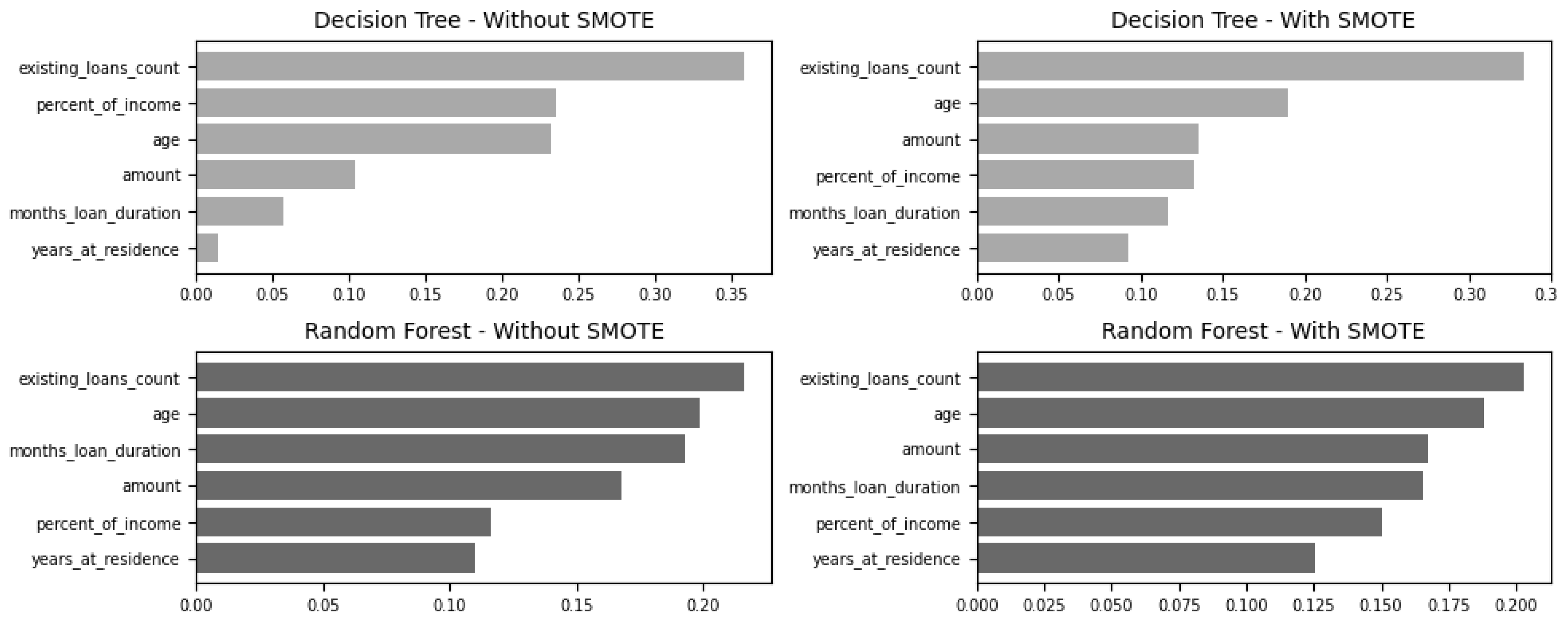
Table 8 shows vast improvements for all five classifiers. Without SMOTE, naïve-bayes is the worst performing classifier with modest improvement alongside logistic regression. However, k-nearest neighbour, decision tree and random forest improve greatly. With imbalanced treatment, k-nearest neighbour improves further. However, the greatest improvement is decision tree which jumps from 0.7726 to 0.9115 followed by k-nearest neighbour which leaps from 0.8227 to 0.9670. What is worth noting, however, is that random forest degrades slightly from 0.9868 to 0.9457. In Permutation-2, both naïve-bayes and logistic regression are indifferent regardless of the inclusion imbalanced data treatment in data pre-processing. The relevant features check (
Figure 7) using the built-in features for decision tree and random forest show the few key features are primarily between “checking balance”, “amount”, “months loan duration”, “age”, “percent of income” and “years of residence.”
Permutation-3 (
Table 9,
Figure 6 and
Figure 8) differs with Permutation-2 in that it further reduces most relevant features from nine to five, where Permutation-2’s nine features are selected by system whilst Permutation-3 is configured to take the best five features. The results are consistent as naïve-bayes and logistic regression are indifferent to imbalanced data treatment whilst k-nearest neighbour and decision tree show big improvements from 0.8221 to 0.8801 and 0.7274 to 0.8206, respectively. The performance for random forest, however, degrades slightly from 0.9677 to 0.9141. In general, the performance of models using the five most relevant features are less optimal than the nine selected by the system.
Finally, comparing with a larger Taiwan credit data set and Permutation-2 (winner),
Table 10 and
Figure 9 and
Figure 10 show that k-nearest neighbour and random forest are the two best performing classifiers across the two data sets. Decision tree performs well in the smaller German credit data set but worse when data is on a larger scale, as in the Taiwan credit data set. Naïve-bayes and logistic regression are indifferent to either smaller or larger data sets, with or without imbalanced data treatment.
7. Conclusions
This study highlights the distinctive characteristics of the five classifiers and how they perform under different data pre-processing steps. The data pre-processing in this study includes data cleansing, features encoding and selection, reduction of dimensions, treatment of imbalanced data and cross validation of training/testing data sets. The final comparisons of the five classifiers demonstrate that data pre-processing steps in conjunction with the data size, complexity and patterns will determine the accuracy of certain classifiers. For example, decision tree performs superbly (overfits) when data size is minor compared to its poor performance when data volume is large. In contrast, the study also shows that random forest does not tend to overfit even with the presence of imbalanced data. In short, the study demonstrates that data distribution and size, multicollinearity, features relevance and imbalanced class contribute to the final scores of models and each classifier reacts to these factors differently (
Table 5).
Equally important is the tuning of the hyper-parameters for respective classifiers, with the study concluding that the default hyper-parameters perform sub-optimally. That being said, investing in computing resources to derive the best hyper-parameters is crucial for striving towards the best performing models and achieving cost savings for lending institutes.
Finally, this study concludes that it is mandatory to apply data domain knowledge prior to selecting a classifier of choice. This is primarily due to fact that a data set may have a pattern that suits one classifier but not the other. Hence, it is imperative to understand by unravelling the complexity and patterns of data sets prior to selecting, training and fitting a model.


