1. Introduction
The classical methods for selecting an investment portfolio, developed by
Markowitz (
1952,
1959) and
Sharpe (
1963), only take into account the market performance of companies, measured by assessing changes in their prices. In the classical model, the potential portfolios of investment are evaluated according to two criteria: expected return (which describes the potential level of profitability from an investment) and risk. The first criterion is measured using the expected rate of return, and the second one using the variance or standard deviation of returns. No other criteria are considered that might give some additional information about the financial standing and prospects of a company that could influence the prices of its shares.
In recent years, however, there has been growing interest in portfolio analysis methods with alternative ways of constructing portfolios. An article by
Kolm et al. (
2014) contains a review of major developments in portfolio theory since its origin, and a book by
Doumpos and Zopounidis (
2014) draws attention to the multicriteria methods used in this field. Most innovations depend on using criteria of risk other than variance or the standard deviation of returns, for example, semi-variance or conditional value at risk. An article by
Fabozzi et al. (
2007) presents a variety of risk measures that are currently used in the practice of portfolio investments. In other approaches, some characteristics of the distribution of returns on assets are used as additional criteria for evaluating portfolio performance. Examples of such characteristics include skewness or kurtosis. Expanded portfolio analysis is presented by
Briec et al. (
2007) and
Rodríguez et al. (
2011).
There are several studies that include criteria that are not based on returns on assets. A branch of the literature takes into account ethical, social, or environmental criteria in portfolio construction, for example, the so-called socially responsible investments approach described in
Steuer et al. (
2007). Articles by
Ballestero et al. (
2012),
Bilbao-Terol et al. (
2013), and
Burchi and Włodarczyk (
2020) are a few more examples illustrating this approach.
Lo et al. (
2003) considered the liquidity of stocks as an additional criterion in the portfolio construction process. There are only a few papers that also take into consideration the fundamental values of companies.
Xidonas et al. (
2010) considered the sum of dividends paid by companies.
Jacobs and Levy (
2013) took into account the risk associated with leverage. The utility function of an investor includes the costs of margin calls, which can force borrowers to liquidate securities at adverse prices due to their illiquidity; losses exceeding the capital invested; and the possibility of bankruptcy.
In accordance with the theoretical concept and empirical research (
Fama and French 1992,
2015,
2017;
Lam 2002;
Zaremba and Czapkiewicz 2017), fundamental factors are important in shaping returns on capital markets. Therefore, it seems rational to include them in a stock portfolio model. The current extensive research on the main financial markets of Eastern Europe has corroborated the significant impact of fundamental information concerning companies on their rates of return. This was also found to hold true for the book-to-market ratio as an indicator of the financial standing of companies. The research sample included five countries: the Czech Republic, Hungary, Poland, Russia, and Turkey (
Zaremba and Czapkiewicz 2017).
There have been several attempts to combine portfolio analysis with the fundamental analysis of companies from the Polish stock markets.
Tarczyński (
2002) developed a synthetic measure to evaluate the economic and financial standing of a company, which he called the taxonomic measure of attractiveness of investment (TMAI), and applied this measure as an additional criterion in the evaluation of possible portfolios. The portfolio constructed using TMAI was called a fundamental portfolio. This model has been modified in recent years, for example, by substituting variance with semi-variance as a risk measure (
Rutkowska-Ziarko and Garsztka 2014). In
Rutkowska-Ziarko (
2013), the Mahalanobis distance was used to determine the TMAI due to the possible correlations between diagnostic financial variables. Another method was proposed by
Pośpiech (
2019) in their research on financial ratios, and market indicators were applied to guide the initial selection of companies.
In this work, in addition to the classic measure of risk (variance), we also used semi-variance. The use of the downside risk measure in choosing an investment portfolio seems to be particularly useful in times of strong declines in the financial markets, such as those in February and March 2020. These were caused by a decline in investor optimism caused by the development of the COVID-19 pandemic. In the calculation of semi-variance, one takes into account only negative deviations below a certain level. Upward deviations, which are connected with higher returns than expected, are not taken into account in determining this measure. Another advantage of semi-variance is that there is no need to make any assumptions about the distribution of rates of return and investors’ utility functions (
Harlow and Rao 1989). The quadratic utility function has some undesirable properties and therefore misrepresents the actual behavior of investors. First, it reaches a maximum for a certain rate of return, and then, its value decreases with an increase in returns, which is in direct contradiction to the preferences of investors, who always prefer to have more than less. Building an effective portfolio for semi-variance is more complicated than the approach in which variance is used as a risk measure. It is impossible to use standard solver software to find a minimum semi-variance portfolio. In the calculation of semi-covariances, one has to know in which periods the rate of return of the entire portfolio was lower than the target value, and this depends on the composition of the portfolio.
This article is organized as follows: After this introduction, in
Section 2, we present a brief description of commonly used market multiples and give some reasons why they could be used as an additional criterion for portfolio choice. In
Section 3, downside risk measures are described.
Section 4 contains a mathematical formulation of portfolio optimization problems and presents the algorithms that were used to solve them.
Section 5 presents the results of empirical research concerning the Polish stock market during the crisis of the COVID-19 pandemic.
2. Market Multiples
Market multiples provide an indication of how the market values a publicly traded company. To calculate the values of these multiples, market data and financial results of a company are used.
Breen (
1968) and
Basu (
1977) analyzed the effect of market multiples on the future profitability of companies. They found that portfolios of companies with lower
P/
E multiples had higher annual returns in the following year than portfolios formed from companies with higher
P/
E multiples. The article of
Basu (
1977) is frequently cited as the first publication in which the impact of market multiples on the future profitability of the companies is analyzed. However, similar research was carried out even earlier, for example, by William
Breen (
1968). He examined companies from index S&P500 indexed over the period from 1953 to 1966, using the COMPUSTAT database. This is a source of fundamental and market information on active and inactive companies and covers around 99% of the world’s total market capitalization. For certain years, equally weighted portfolios (of 10 and 50 companies) were constructed using the stocks of companies with the lowest and highest
P/
E multiples. The results indicate that portfolios built with stocks of companies with lower
P/
E multiples had higher annual returns in the following year than portfolios built with stocks of companies with higher
P/
E multiples.
Barbee et al. (
2008) investigated the impact of market multiples values on future prices of stocks. They analyzed the profitability of equally weighted portfolios built using the shares of companies with various values of different market multiples.
The most popular indicator of the market’s valuation of a company is the
P/
E multiple, which relates the earnings per one ordinary share to its market price:
In this study, four different measures of the ability of a company to generate profit were considered: net profit (EAT); gross profit (GP); earnings before interest, taxes, depreciation, and amortization (EBITDA); and operating profit (EBIT).
Net profit is the last position in the Profit and Loss Account, it is calculated as follows:
Gross profit is earnings before taxation. EBITDA is earnings before interest, taxes, depreciation, and amortization. EBITDA can be used to describe a company’s financial performance without taking into account its capital structure. The operating profit is an accounting measure that measures the profits that a company generates from its operating activities. Interest and taxes are not considered here.
One can relate a share price not only to different profit categories but also to other characteristics that describe the economic situation of a company. It may be important for an investor to relate the market valuation of the company’s share capital to the net value of its assets. The
P/
BV multiple relates the price of an ordinary share to the book value of the company, estimated per ordinary share. This multiple shows the market value of the company in relation to its book value.
where
The book value refers to the total amount the company would be worth if it liquidated its assets and paid back all its liabilities, and it is also the net asset value of the company.
A positive relationship between the book-to-market ratio and average returns was described by
Rosenberg et al. (
1985). This phenomenon was also observed in Japanese stocks (
Chan et al. 1991). Based on this research,
Fama and French (
1992) suggested that the book-to-market ratio would be an important risk factor explaining the variability of stock rate of returns.
In this paper, instead of using classical market multiples, we used their reciprocals, i.e., the values of financial indicators (expressed per one share) divided by the current market price of a share. The reason is the additivity of such indicators. The value of these indicators for the portfolio as a whole is a weighted average of the values of the indicators of individual companies. Thus,
is replaced by the book-to-market ratio (
:
The same was used for the
P/
E multiple, in fact, for the whole group of market multiples based on various methods for calculating the company’s profits. Instead of the price-to-equity ratio, the earnings-to-price ratio (
E/
M) was used, calculated using the equation below:
3. Downside Risk in Portfolio Choice
In portfolio theory, variance has been a commonly used measure of risk in capital market analysis from its inception to the present day (
Markowitz 1952). At the same time, there have been doubts about the validity of using this risk measure for almost as long (
Markowitz 1959). The main disadvantage of variance as a measure of risk is that it treats negative and positive deviations from a mean return in the same way. In fact, negative deviations are undesirable, and positive deviations create an opportunity for greater profit. To measure only negative deviations,
Markowitz (
1959) proposed semi-variance, which is an average of deviations below a certain level. Semi-variance and lower moments consider only the variability on the left side of a distribution. The reference point can be the mean, as in the case of variance, but another value can also be used as the reference point. Using semi-variance as a measure of risk is consistent with investors’ intuitive perception of risk (
Boasson et al. 2011).
Variance is assumed to be an appropriate risk measure when the distribution of returns is normal, or at least symmetric, or when an investor has a quadratic utility function. The classical Markowitz model (
Markowitz 1952) is ineffective in selecting portfolios that comprise assets with skewed returns. The traditional mean–variance model, which treats deviations above and below the target return equally, tends to overestimate risk and imposes unnecessary conditions that exclude portfolios that are downside efficient.
Pla-Santamaria and Bravo (
2013) constructed portfolios of blue-chip stocks from the Dow Jones Industrial Average. Their results show significant differences between the portfolios obtained by mean–semi-variance efficient frontier model and those with the same expected returns obtained using the classical Markowitz mean–variance efficient frontier model.
An investor who does not wish the return of their portfolio to fail below the target rate of return would tend to compose portfolios that minimize downside risk measures (
Klebaner et al. 2017).
It is believed that, in symmetrical distributions, variance as a risk measure is no worse than semi-variance (
Estrada and Serra 2005;
Galagedera and Brooks 2007). However, research on capital markets shows that the distributions of rates of return of many companies are not normal or at least symmetrical (
Adcock and Shutes 2005;
Estrada and Serra 2005;
Markowski 2001;
Post and van Viet 2006;
Sun and Yan 2003). Then, the use of lower-risk measures becomes important. In the case of right-skewed distributions of returns, the main part of the variance includes upper deviations, which mean the achievement of high returns. The impact of lower deviations is relatively small. For this reason, investors are looking for companies with right-skewed distributions of returns (
Galagedera and Brooks 2007;
Peiro 1999), which suggests that the issue of skewness cannot be ignored in the risk analysis, even if the distribution of the returns of some companies are symmetrical. Also, according to the perspective theory (
Kahneman and Tversky 1979), it is more appropriate to use semi-variance instead of variance as a risk measure.
The above arguments speak in favor of lower-risk measures when compared with their classic counterparts. Lower-risk measures, such as a semi-variance, allow for a universal approach to risk analysis and equity portfolio construction, regardless of the empirical distribution of returns. One also does not have to assume a specific analytical form of the utility function. It is sufficient to make the obvious assumption that an investor prefers to earn more than less, and therefore higher rates of return are better than lower rates of return.
A semi-variance, defined by
Markowitz (
1959), is a lower counterpart of a variance. This lower-risk measure is the sum of the squared of lower deviations from the target rate of return
. It is calculated using the following formula:
where
—Rate of return of company in period ;
—Semi-variance for company ;
—The number of time periods;
—The mean rate of return or any target rate of return chosen by an investor.
Extensions of semi-variance as a risk measure are lower partial moments, introduced by
Bawa (
1975) and
Fishburn (
1977). According to these authors, the lower partial moment of order
is given by
where
Notice that for , the lower partial moment is equal to semi-variance.
The semi-variance of an investment portfolio
is given by
where
is the share of stock
in the portfolio, and
is the semi-covariance of the rate of return for the
i-th and the
j-th shares, which is defined by
where
4. Problems Related to Portfolio Choice
We consider a portfolio of
different assets. Let
be a mean return of an asset
, estimated from the last
observations of
where
denotes a covariance between the returns of asset
and asset
:
where
denotes the proportion of the wealth invested in asset
. The mean return of the portfolio is then given using the following formula:
and the variance of the portfolio’s rate of return is given by
The semi-variance of the portfolio form given by
where semi-covariances of assets’ returns are given in (1).
We assume that some market multiples are also considered. It can be connected with the book-to-market value per share or with the earnings-to-price ratio of a share. Let
denote the value of this criterion for the asset
. The value of this multiple for the whole portfolio is given by
In the empirical part of the work, we consider portfolios that are the solutions to the following optimization problems:
A portfolio minimizing the variance, i.e., a portfolio that is the solution of
with the constraint that
A portfolio that minimizes variance with a constraint on the mean return: In this case, we assume that the mean return of the portfolio should be no smaller than the required rate of return
. The optimization problem is given in (2)–(4) with an additional constraint.
A portfolio that minimizes variance with constraints on the mean return and its fundamental value: We assume that the fundamental value of the portfolio (measured with one of the market multiples) should not be lower than its required value
. In the empirical part of this study, we assume that the minimal value of the portfolio multiple should be equal to the average of the multiples for all the companies considered. This yields problems (2)–(5) with an additional constraint.
Mathematically, variance minimization problems are problems of quadratic optimization problems with linear constraints, which are determined using equations and inequalities. They can be solved using standard algorithms. We solved them using the method of
Goldfarb and Idnani (
1983) implemented in the R package quadprog.
The second set of portfolios are those that were optimized with the use of semi-variance as a measure of risk. The optimization problems were defined as follows:
A portfolio minimizing the unconditional semi-variance, i.e., a portfolio that is the solution of
with the constraints determined using (3) and (4).
A portfolio minimizing semi-variance with a constraint on mean return, which should be no lower then : the optimization problem is given with the set of conditions in (7) and (3)–(5).
A portfolio that minimizes semi-variance with a constraint on mean return and its fundamental value: the optimization problem is given with the set of conditions (7) and (3)–(6).
To solve these problems, the following numerical algorithm was used: We started with an initial portfolio (in this case, it was a portfolio minimizing variance). Then, we solved each of the problems as a problem of quadratic programming, using the
Goldfarb and Idnani (
1983) method. After each iteration, we re-estimated semi-covariances
and solved the problems with the new input data. We repeated this process until convergence, i.e., until changes in the portfolio structure between each iteration were sufficiently small. In the calculations, we used procedures written in R and the R package quadprog.
5. Data and Empirical Results
The studies covered 20 of the largest and most liquid companies listed on the Warsaw Stock Exchange, excluding financial companies. Close share prices from the period 1 April 2016–4 September 2020 were taken for analysis. In the estimation, we assessed the portfolios using their monthly rate of returns. The parameters (mean returns, variances, and semi-variances) used in constructing the portfolios investigated in this research were estimated using a period of three years before the start of an investment. Figures from financial statements were used, namely the net profit (EAT); the gross profit (GP); earnings before interest, taxes, depreciation, and amortization (EBITDA); the operating profit (EBIT); and the book value (BV). They changed with the publication of the quarterly financial statements of the companies. We calculated the appropriate indicators for each company according to its financial statement. For the calculation of financial indicators, we always used the latest available data, according to the date of publication. We considered the financial statements for the period from Q3 2019 to Q2 2020. Information on financial results is usually published with a delay of 60 to 120 calendar days. It was assumed that portfolios purchased on a given day were sold after a month (four weeks). The data were taken from the Thomson Reuters database—Refinitiv Eikon.
In economics, it is not possible to carry out repetitive experiments, as in, for example, physics or chemistry. Thus, in this article, the COVID-19 pandemic was used as a natural experiment. During the pandemic, there was a sharp collapse in stock exchanges, which allows us to test the usefulness of various risk diversification methods in times of sharp drops in prices in financial markets.
In this paper, we considered 15 types of portfolios.
Table 1 lists the descriptions of these types and the symbols used to refer to them.
Altogether, we developed 2655 portfolios during 177 trading days. We assumed that the investment period is one month. However, to assess the performance of the strategies, we calculated portfolios for each trading day. Thus, the first analyzed set of portfolios was created on 21 November 2019, and its performance was calculated based on one-month returns (i.e., price changes until 19 December 2019). The next set of portfolios was created on the next trading day (22 November 2019), and the performance was evaluated based on price changes until 20 December 2019, etc.
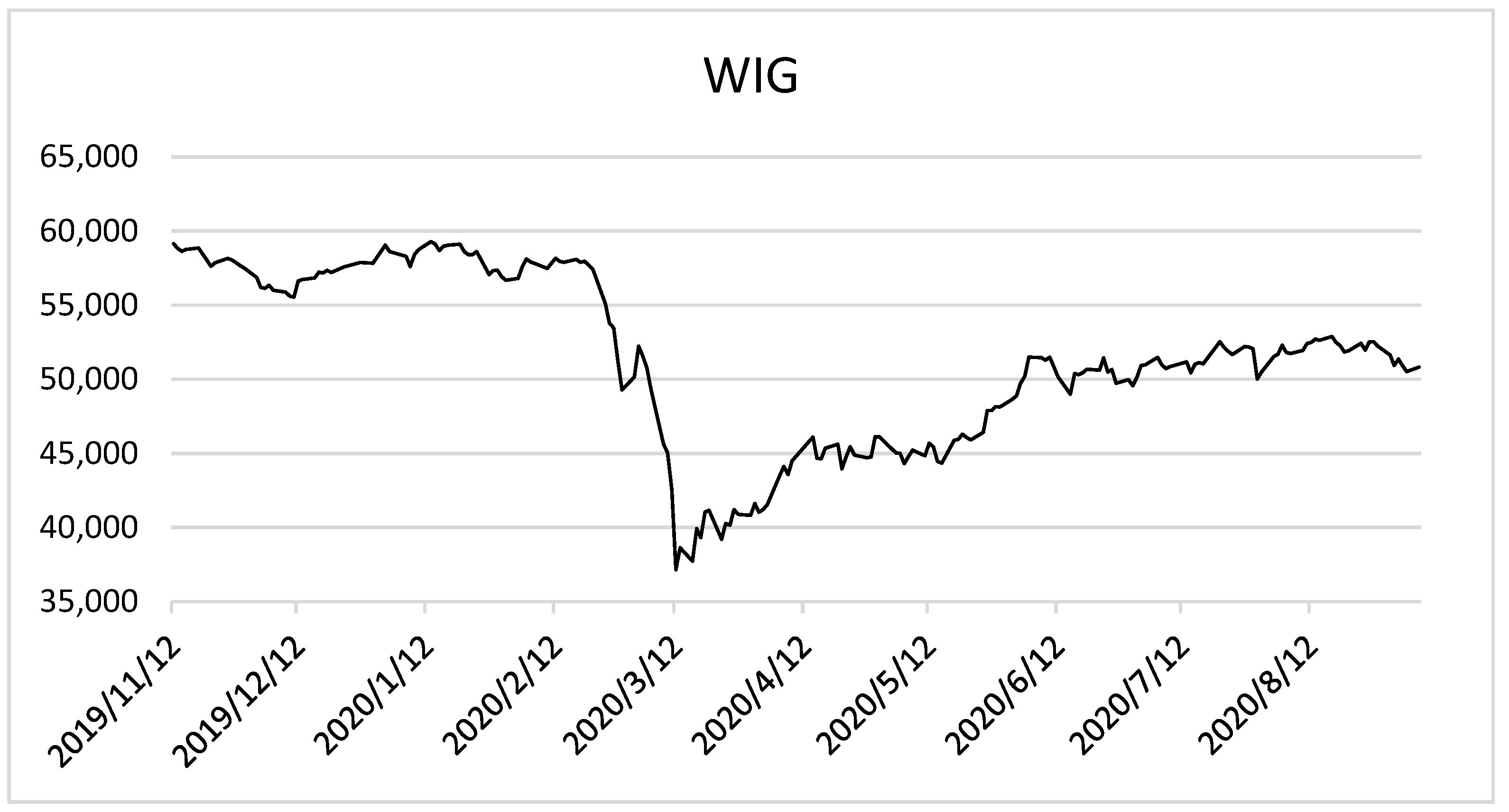
During the research period, four research subperiods of different lengths were specified. The division criterion was the changes in the situation of the capital market, which was reflected in the changes in the values of the WIG Index, the main index on the Warsaw Stock Exchange. The key aspect for identifying subperiods was the situation of the market during buying and selling a portfolio.
Table 2 outlines the descriptions of the subperiods.
Due to the very large number of the considered portfolios (2655), in this study, we omitted the factors related to the structure of these portfolios and other elements of ex ante analysis, such as the expected portfolio risk, the average rate of return, or the average market ratio. All the characteristics of the distribution of return presented in
Table 3,
Table 4,
Table 5,
Table 6 and
Table 7 refer to realized returns. That is, they describe the actual returns of investors, as well as the risk they bear. For the individual subperiods and the entire research period, the following characteristics were calculated: the mean rate of return, the minimal rate of return, the value-at-risk (VaR) measure, semi-deviation, standard deviation, and skewness.
In the first research subperiod, the negative effects of the COVID-19 pandemic had not yet affected the Polish stock market. We observed that all the portfolios minimizing the semi-variance had right-skewed distributions of rates. Returns of equally weighted portfolios and portfolios minimizing the variance were left-skewed. The highest average rate of return occurred for portfolios minimizing semi-variance and with a fundamental criterion. However, it is difficult to unequivocally determine which type of diversification was the most effective in reducing the risk during this period.
At the end of January 2020, the financial markets collapsed, and this situation lasted until mid-March. It affected not only Poland but practically all the most important world exchanges. During this period, all average rates of return were negative. The least effective strategy at this time was to select an equally weighted portfolio. It was the least profitable and the riskiest one, taking into account, among others, VaR 0.1, VaR 0.05, and semi-deviation. The most secure and at the same time most profitable portfolios were fundamental portfolios that minimized semi-variance. The distributions of the realized returns were right-skewed (with only one exception for the portfolio minimizing variance), but the strength of this asymmetry was small.
In the third subperiod, the quotations of the WIG Index slowly began to rise. During this period, purchasing an equally weighted portfolio proved to be a fairly effective method of risk diversification. The highest average rates of return, as in the second subperiod, were achieved using fundamental portfolios that minimized semi-variance. It is worth noting that the portfolios minimizing the semi-variance had higher values of this risk measure than the portfolios minimizing the variance. At the same time, portfolios minimizing the variance had higher realized variances. However, taking into account extreme values such as minimal return, VaR 0.05, and VaR 0.01, there is a clear advantage of portfolios with minimized semi-variance. In the third subperiod, all portfolios were characterized by right-hand asymmetry, which was stronger than in the second subperiod.
In the fourth subperiod, the Warsaw Stock Exchange stabilized, and price increases were small, as it is shown in
Figure 1. The realized rates of return for equally weighted portfolios and those with minimum semi-variance were generally characterized by left-hand asymmetry, and those with minimum variance were characterized by right-hand asymmetry. During this period, for many fundamental portfolios, the condition imposed on a given market ratio for the portfolio was not active, especially for market ratios based on various measures of a company’s profitability.
Over this period, the most profitable portfolios were those selected according to the minimum variance criterion. The average rate of return for the equally weighted portfolios was quite high, and the risk was lower than in Markowitz portfolios. In the fourth subperiod, advanced models of building stock portfolios had similar usefulness for stock exchange investors as the simple method of selecting an equally weighted portfolio.
In the entire research period (
Table 7), portfolios with three criteria (average return, risk, and a fundamental criterion) allow for achieving higher realized returns than equally weighted portfolios, portfolios minimizing risks (measured either with the variance or semi-variance), or average return–risk portfolios. Additionally, it can be seen that the introduction of a fundamental criterion reduced the risk borne by an investor, measured with both standard deviation and semi-deviation. An analysis of extreme values (minimum return, VaR 0.1, and VaR 0.05) also shows the advantage of fundamental portfolios. As can be seen, the whole group of portfolios minimizing semi-variance was characterized by a lower ex post risk than those minimizing variance. Fundamental portfolios had less left asymmetry, especially for portfolios that were designed to minimalize semi-variance. It should be emphasized that having less left asymmetry is beneficial for investors, as it means they are less exposed to very low rates of returns.
In order to test whether there were differences in returns between the different portfolio selection methods, we performed appropriate statistical tests. Since the realized returns were not normally distributed (which we evaluated using the Shapiro–Wilk test and the Jarque–Bera test) we used the nonparametric Kruskal–Wallis test with post hoc Dunn’s test to determine the differences between each pair of the portfolios. To assess the differences, we used the realized returns for the different types of portfolios from the entire research period. The test statistics for the Kruskal–Wallis test was 21.64, which indicates that the hypothesis of equal mean returns should be rejected, with a
p-value lower than 0.1 (
p-value = 0.086). This result shows that there were differences in the distributions between different groups of the realized returns. To analyze these differences, we carried out a post hoc analysis based on Dunn’s tests, in which we assessed each pair of groups.
Table 8 shows the results of these tests. A statistical difference was observed between the returns of equally weighted portfolios (i.e., portfolios constructed without using any theoretical methods) and portfolios that minimized the semi-variance. The semi-variance-minimizing portfolios were also statistically superior to the variance-minimizing portfolios.
6. Conclusions
This paper involves the development of fundamental portfolios using both variance and semi-variance approaches. An iterative algorithm written in R software (R.4.3.1) was used to construct the portfolios in the semi-variance framework.
For fundamental portfolios, three criteria were considered: profitability (measured with the expected return), risk (measured using the variance or semi-variance of returns), and the market ratio of the companies in the portfolio. Five different market ratios were used in this study. The usefulness of portfolio selection models during the COVID-19 pandemic was analyzed. This period was divided into four subperiods due to the changing situation of the Warsaw Stock Exchange.
During this period characterized by the collapse of the financial market, the worse strategy was to select an equally weighted portfolio. It was the least profitable and the most risky one, taking into account, the value-at-risk measure and semi-deviation. It can be seen that the safest and at the same time most profitable portfolios were fundamental portfolios that minimized semi-variance.
Throughout the entire period under review, the portfolios with three criteria (average return, risk, and a fundamental criterion) allowed higher realized returns to be achieved than equally weighted portfolios, portfolios minimizing the risk (measured using either the variance or semi-variance), or the average return–risk portfolios. In addition, it was found that the introduction of the fundamental criterion reduced the risk borne by an investor, measured with both standard deviation and semi-deviation. The analysis of the value-at-risk measure also shows the advantage of fundamental portfolios. It was revealed that the whole group of portfolios that minimized semi-variance were characterized by a lower ex post risk than those that minimized the variance.
The empirical research for the largest companies traded on the Warsaw Stock Exchange reveals the following findings:
Investors can obtain better investment results by adding a criterion associated with market ratios, such as book-to-market or earnings-to-market ratios, to the Markowitz model;
The use of semi-variance instead of variance yields better results for investors, as can be clearly seen in the period of the collapse of the capital market;
Fundamental portfolios with minimum semi-variance seem to be a useful tool to choose an investment strategy during the COVID-19 pandemic.


