

A Study about Who Is Interested in Stock Splitting and Why: Considering Companies, Shareholders, or Managers

Abstract
:1. Introduction
2. Literature Review
2.1. On Hypothesis 1: To Attract More Shareholders
- to make it more convenient for small stockholders to purchase round lots;
- to keep the firm’s stock price within an optimal price range;
- to increase the number of shareholders;
- to make stocks more attractive to new investors or speculators.
“The clientele preferring a lower price range is usually thought to be uninformed or small investor.”
2.2. On Hypothesis 2: To Level off Information Asymmetries on Firm Value
2.3. On Hypothesis 3: To Provide Stock Splits/Dividends, New Shares, and Liquidity
3. Methodology
3.1. The Research Method for Hypothesis 1
3.2. The Research Method for Hypothesis 2
- Steps for calculating the return:
- 1.1.
- Identify the adjusted closing price on the first and last day of the period before the split.
- 1.2.
- Divide the adjusted closing price at the end of the period by the one at the beginning of the period. This gives the “normal return rate”.
- 1.3.
- Then, find the index’s adjusted closing price on the first and last day of the period after the split.
- 1.4.
- Divide the ending adjusted closing price by the beginning adjusted closing price.
- 1.5.
- Multiply the stock’s beta. This gives the return rate after the split has influenced the market.
- 1.6.
- Subtract the two results; the difference value shows whether the stock generates better returns than expected.
- Steps for calculating beta:
- 2.1.
- Calculate the percent change period to period for both the stock price rate (rsf) and the risk-free rate (rf).
- 2.2.
- Find the Variance of the stock price
- 2.3.
- Find the Covariance of the stock price to the risk-free rate.
- 2.4.
- Use this formula to calculate beta: .
3.3. The Research Method for Hypothesis 3
4. Data Selection and Description
- The language of the annual report is not English;
- There are different standards in annual reports;
- There are no historical yearly report documents remaining on the homepage;
- We were incapable of collecting the full data of interest.
5. Results
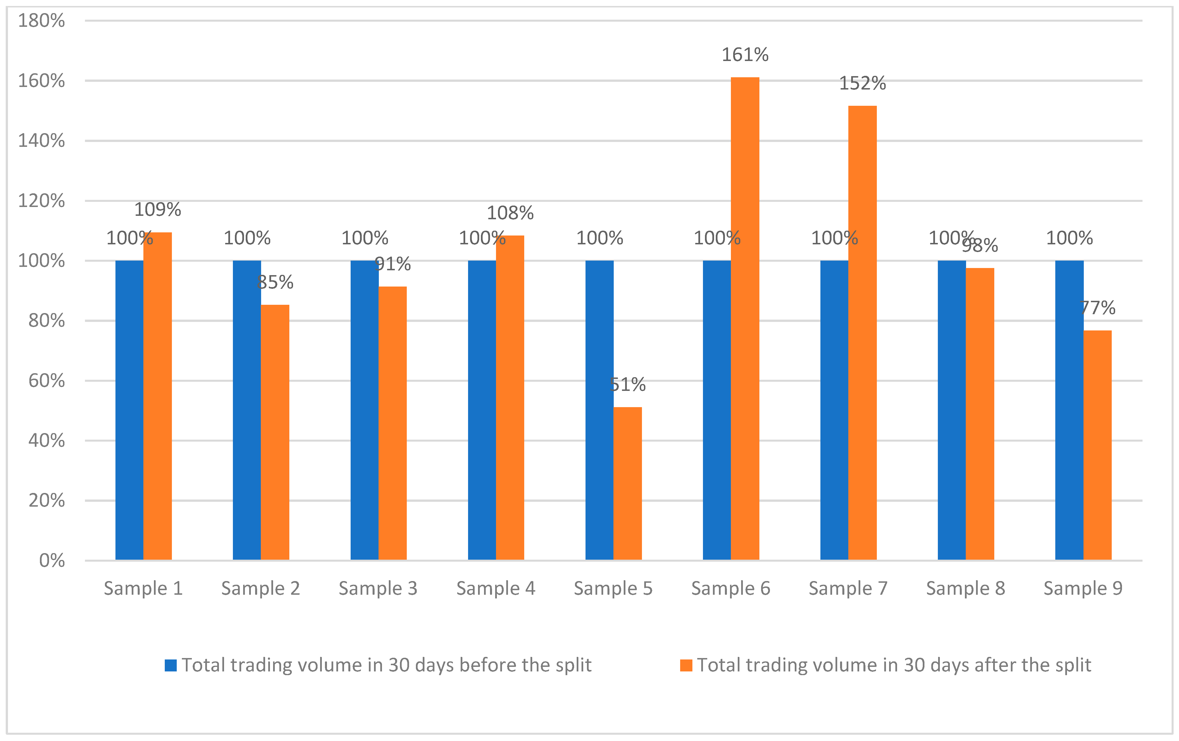
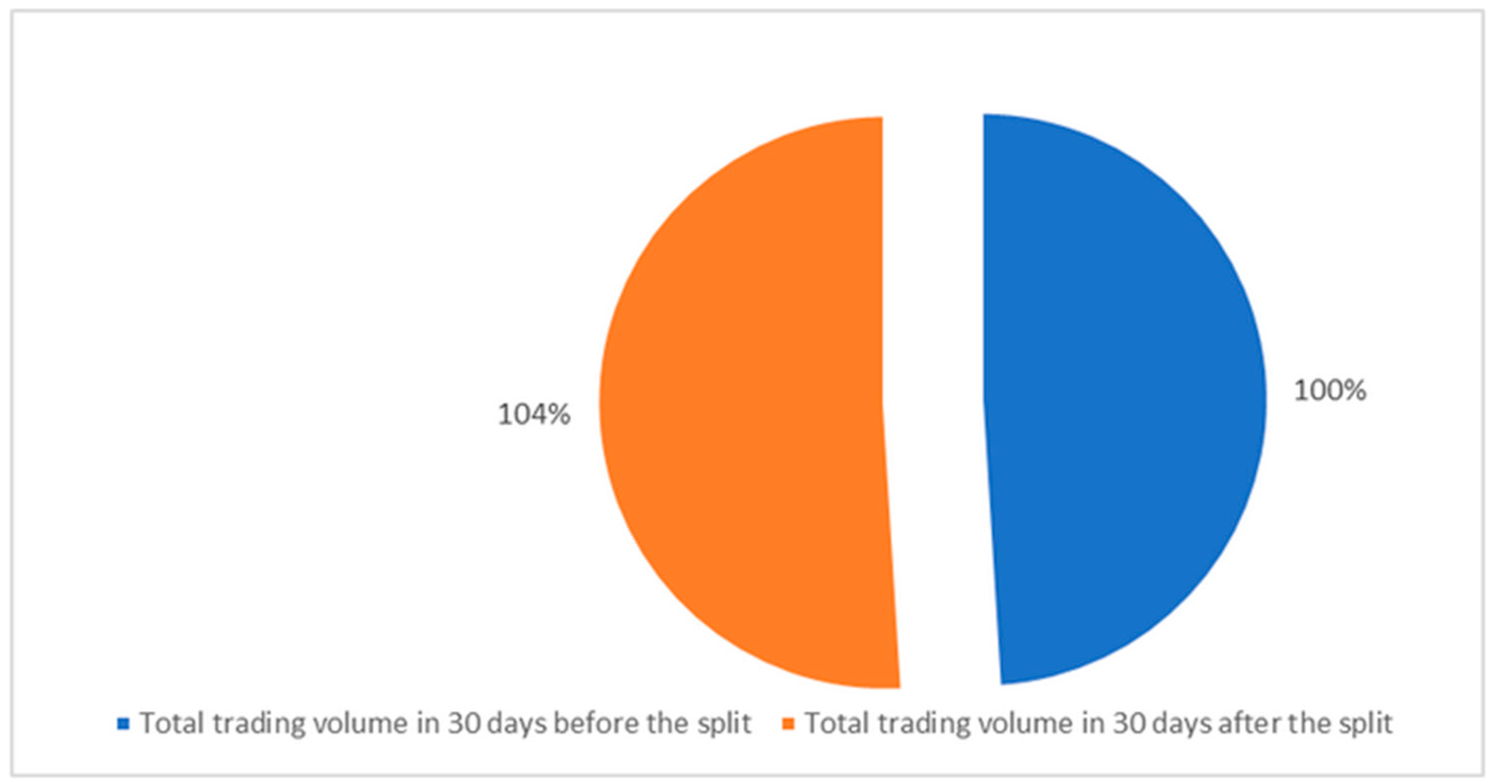
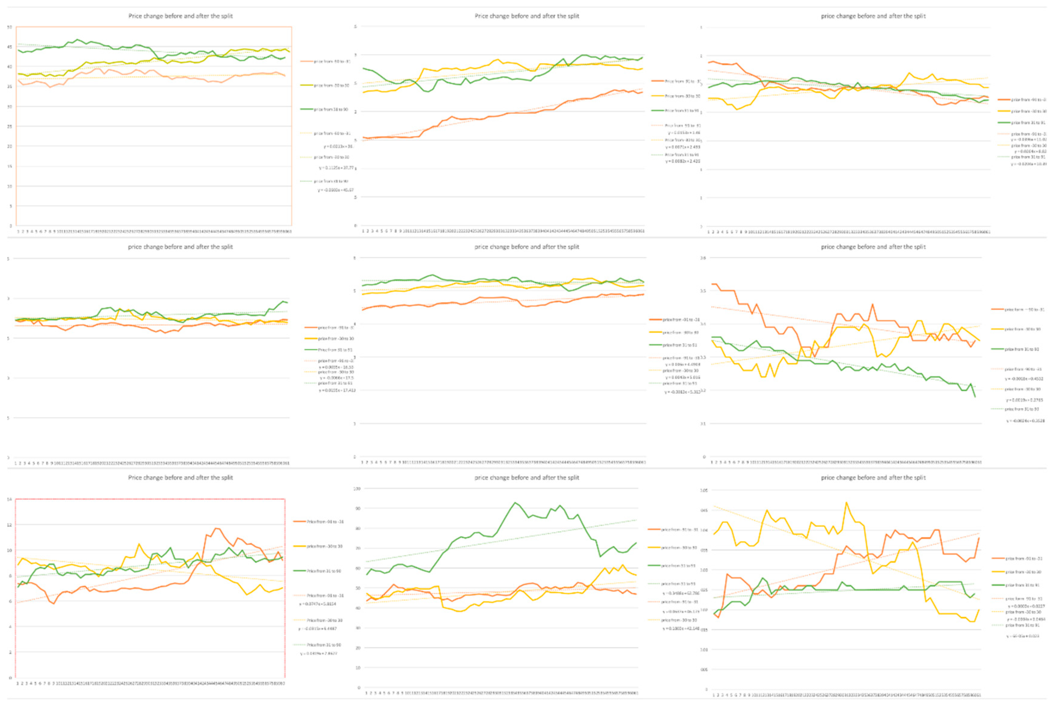
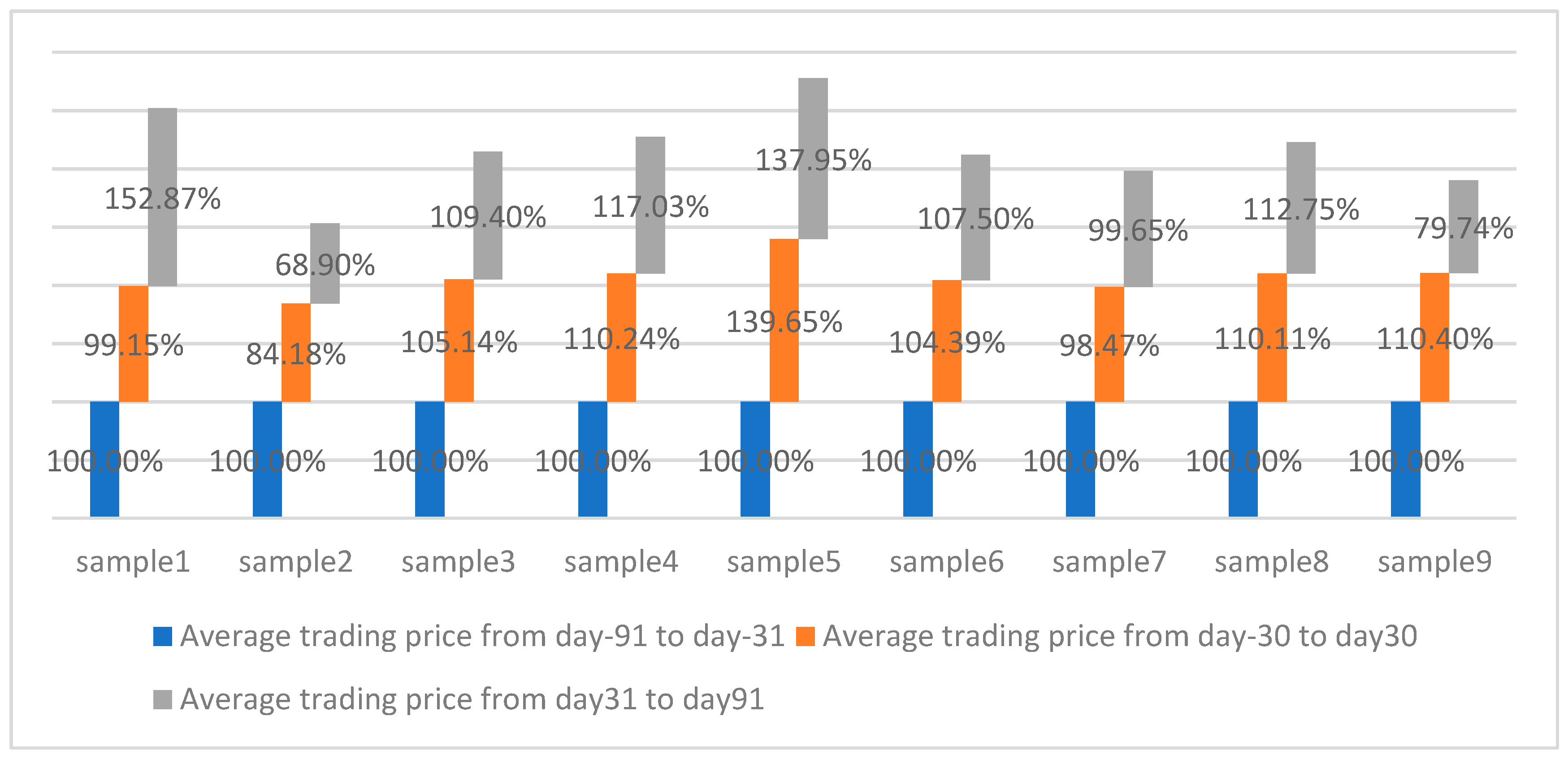
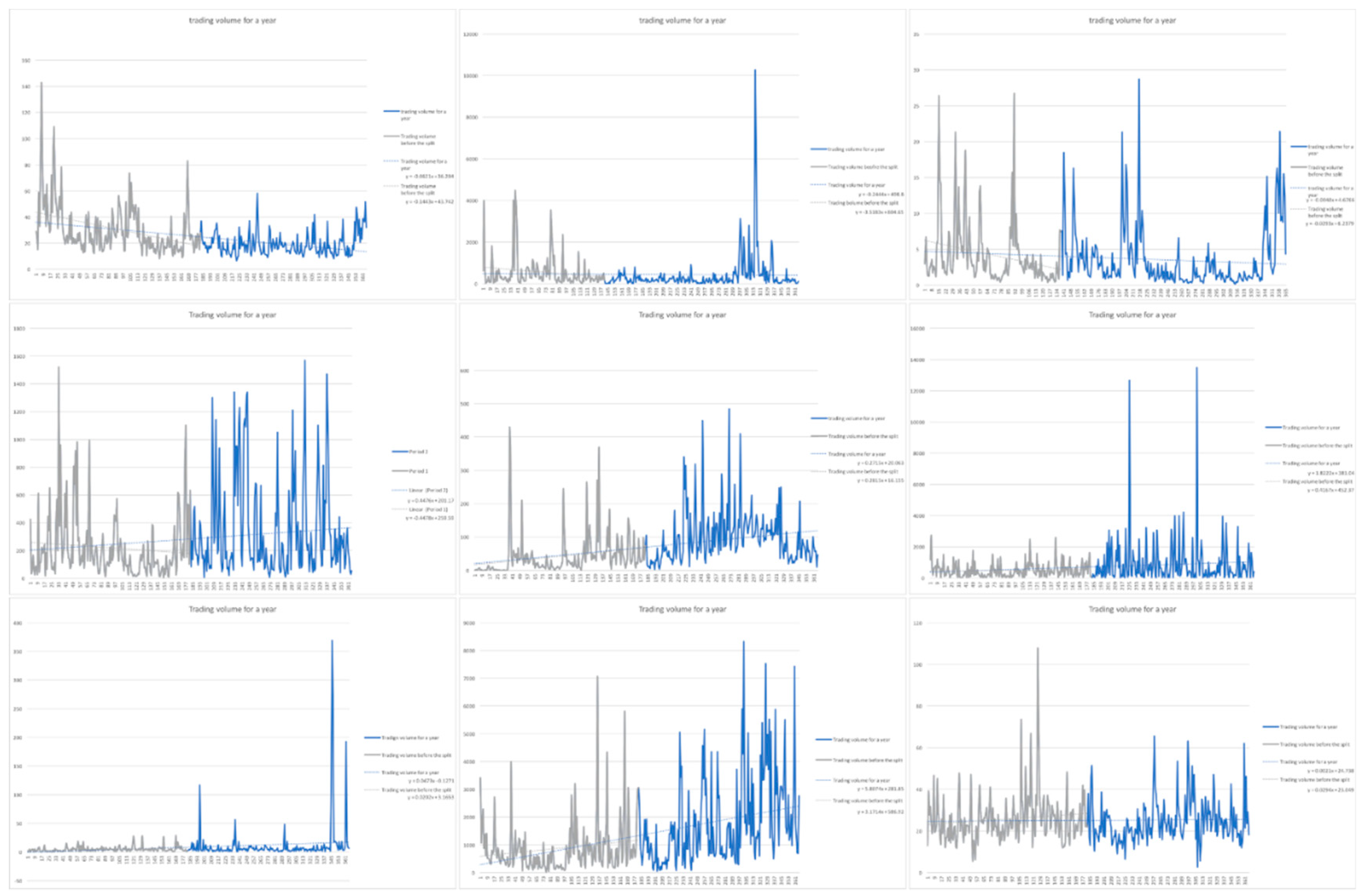
5.1. Hypothesis 1
- Stock split events have a slight impact on the market.
- There is an unexpected increase in trading volume for some samples, but “on average”, there is none.
- There was an explosive demand for shares.
- Investors are unwilling to trade their shares little by little after the split date.
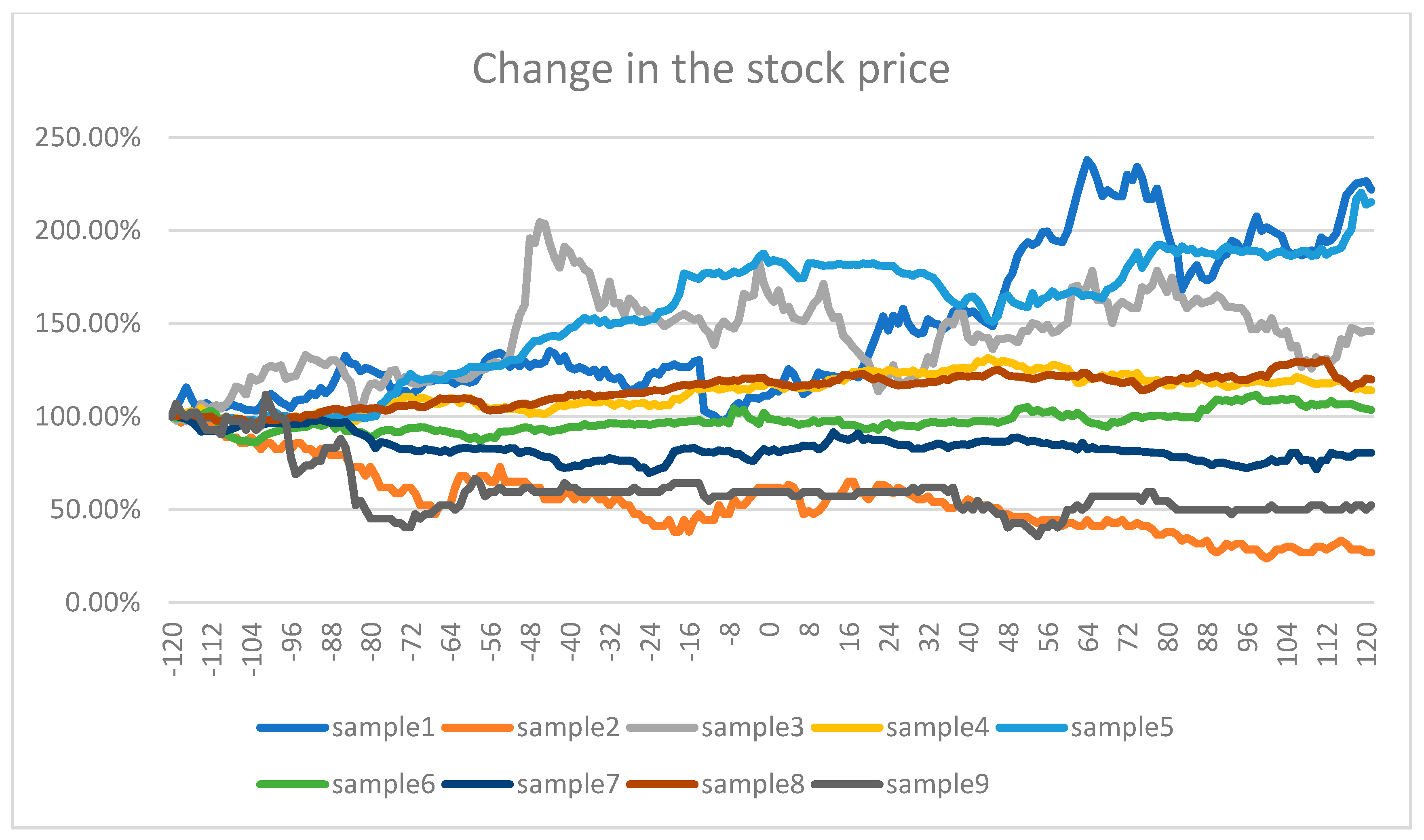
- The stock price after the split is higher than the price before the split.
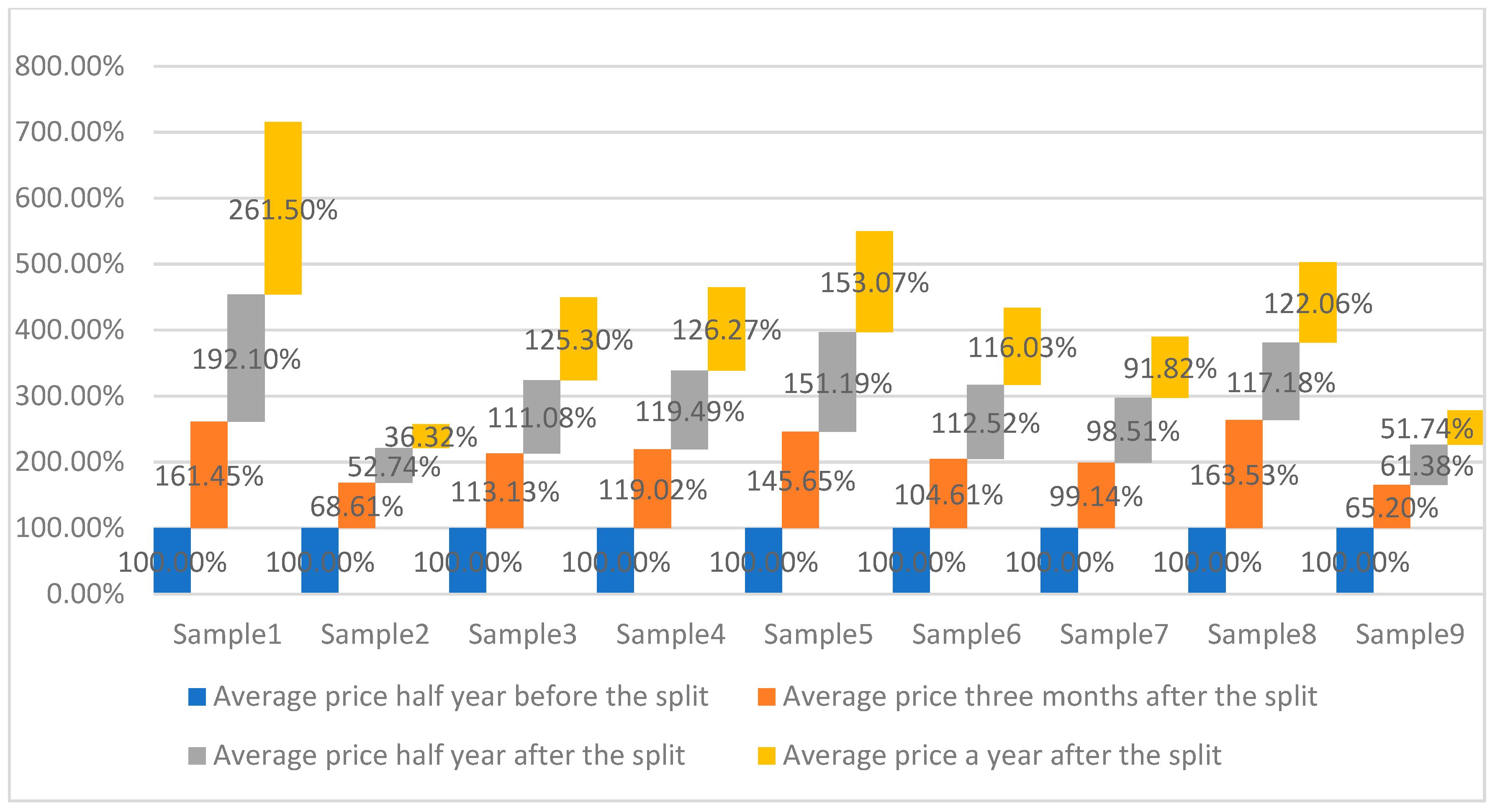
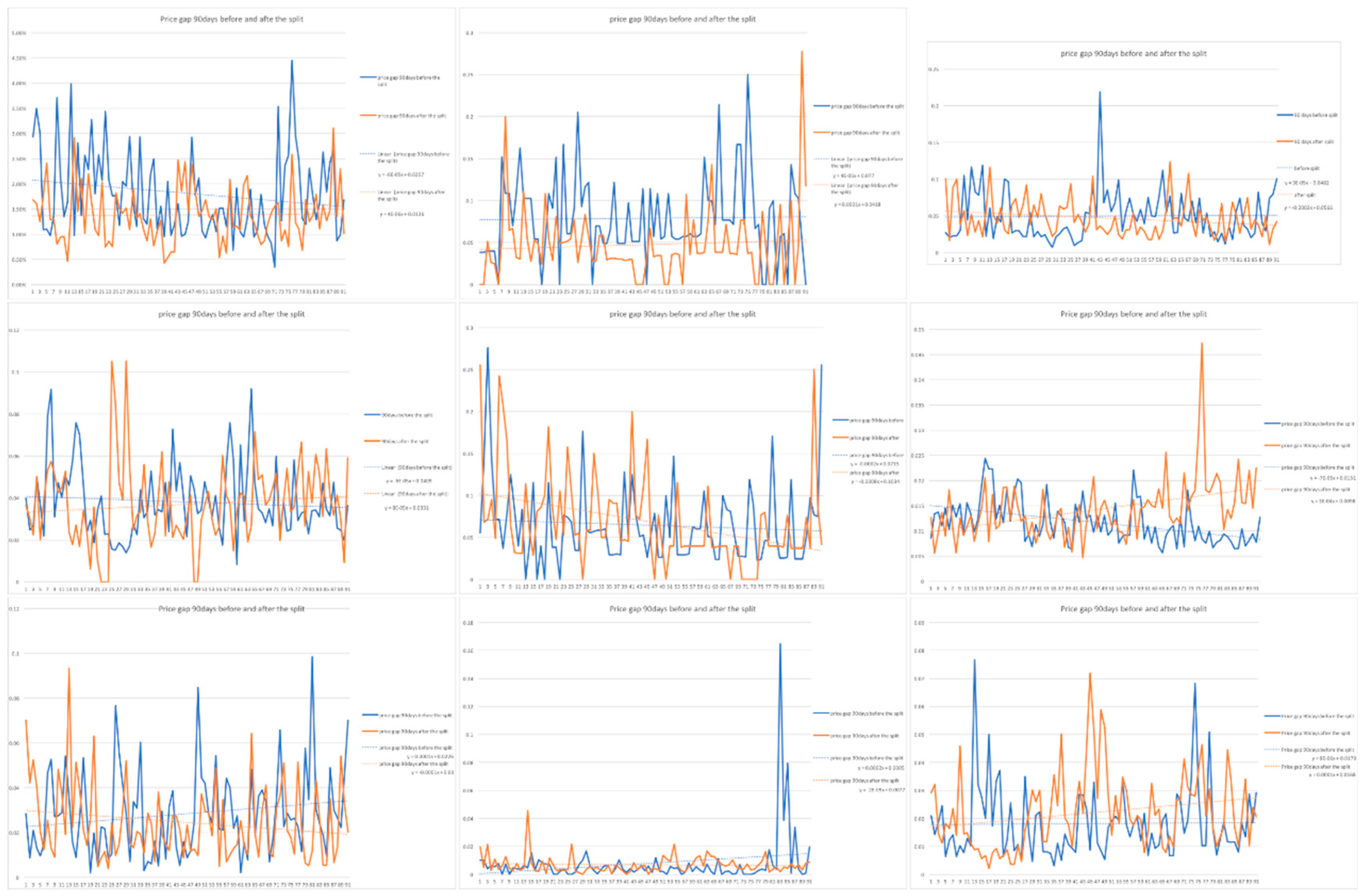
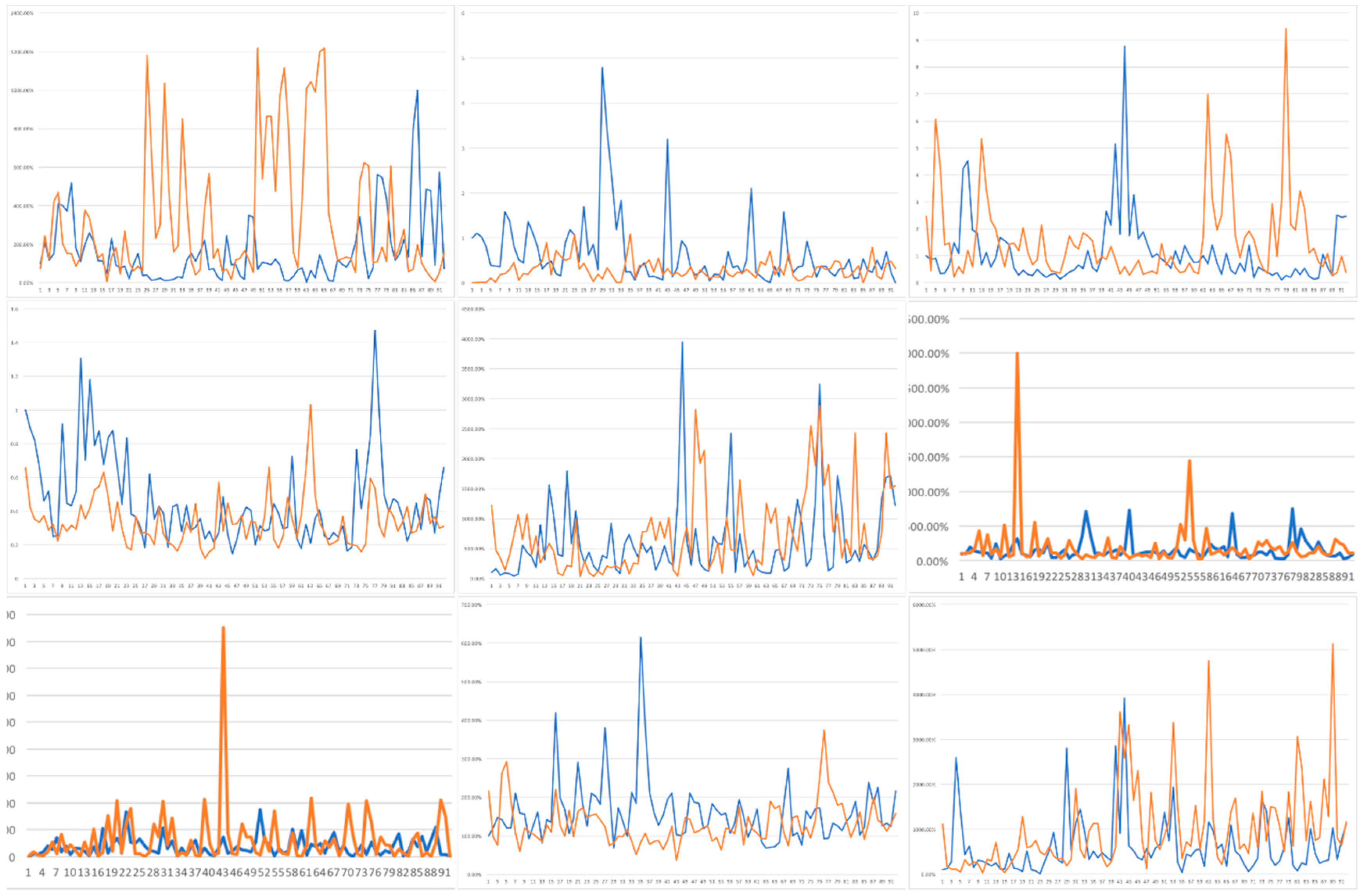
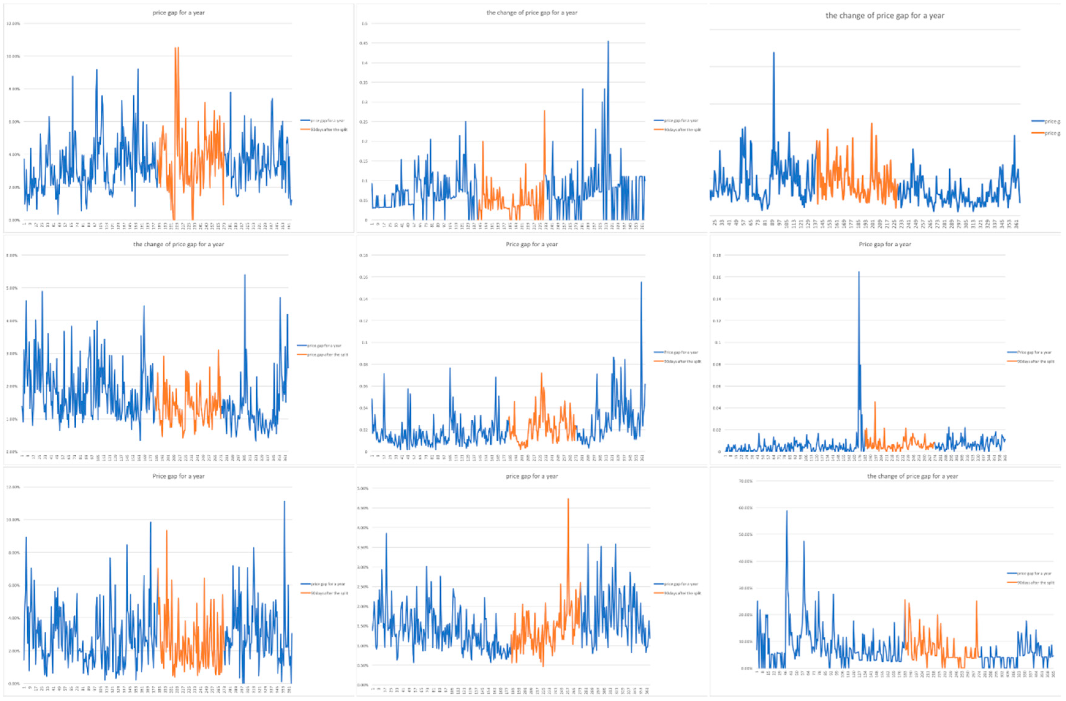
5.2. Hypothesis 2
- P1: The stock price before the stock split;
- P2: The stock price after the stock split;
- N1: The number of shares before the stock split;
- N2: The number of shares after the stock split;
- V1: The market value of the sample before the stock split;
- V2: The market value of the sample after the stock split;
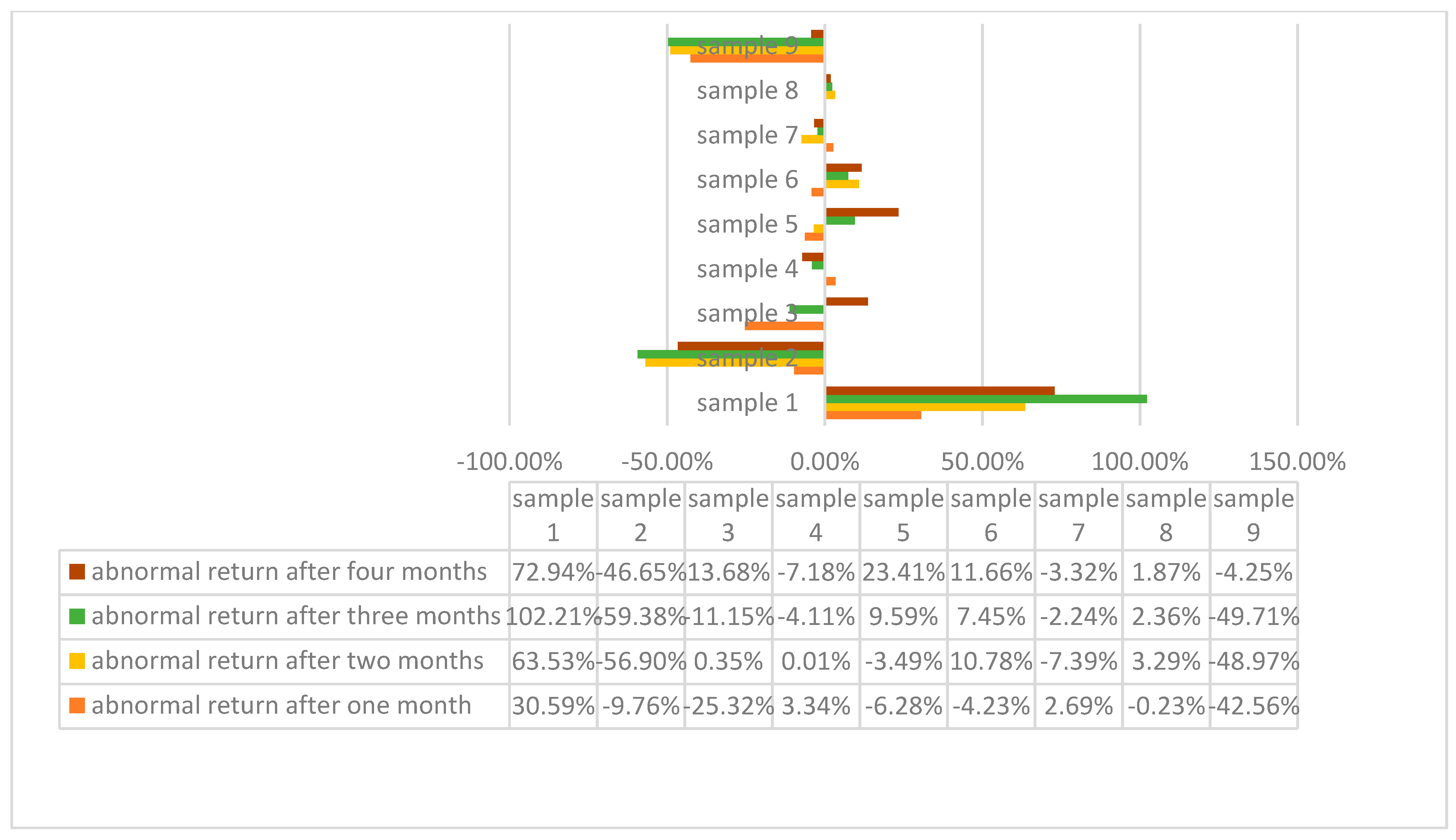
- After the first month, investors of sample 1, sample 4, and sample 7 could receive 30.59%, 3.34%, and 2.69% abnormal earning separately.
- After two months, investors of sample 1 (63.53%), sample 3 (0.35%), sample 4 (0.01%), sample 6 (7.45%), and sample 8 (3.29%) could gain abnormal earnings.
- After a season, investors of sample 1 (102.21%), sample 5 (9.59%), sample 6 (7.45%), and sample 8 (2.36%) could obtain an abnormal return.
- After four months, investors of sample 1 (72.94%), sample 3 (13.68%), sample 5 (23.41%), sample 6 (11.66%), and sample 8 (1.87%) will get the extra earnings.
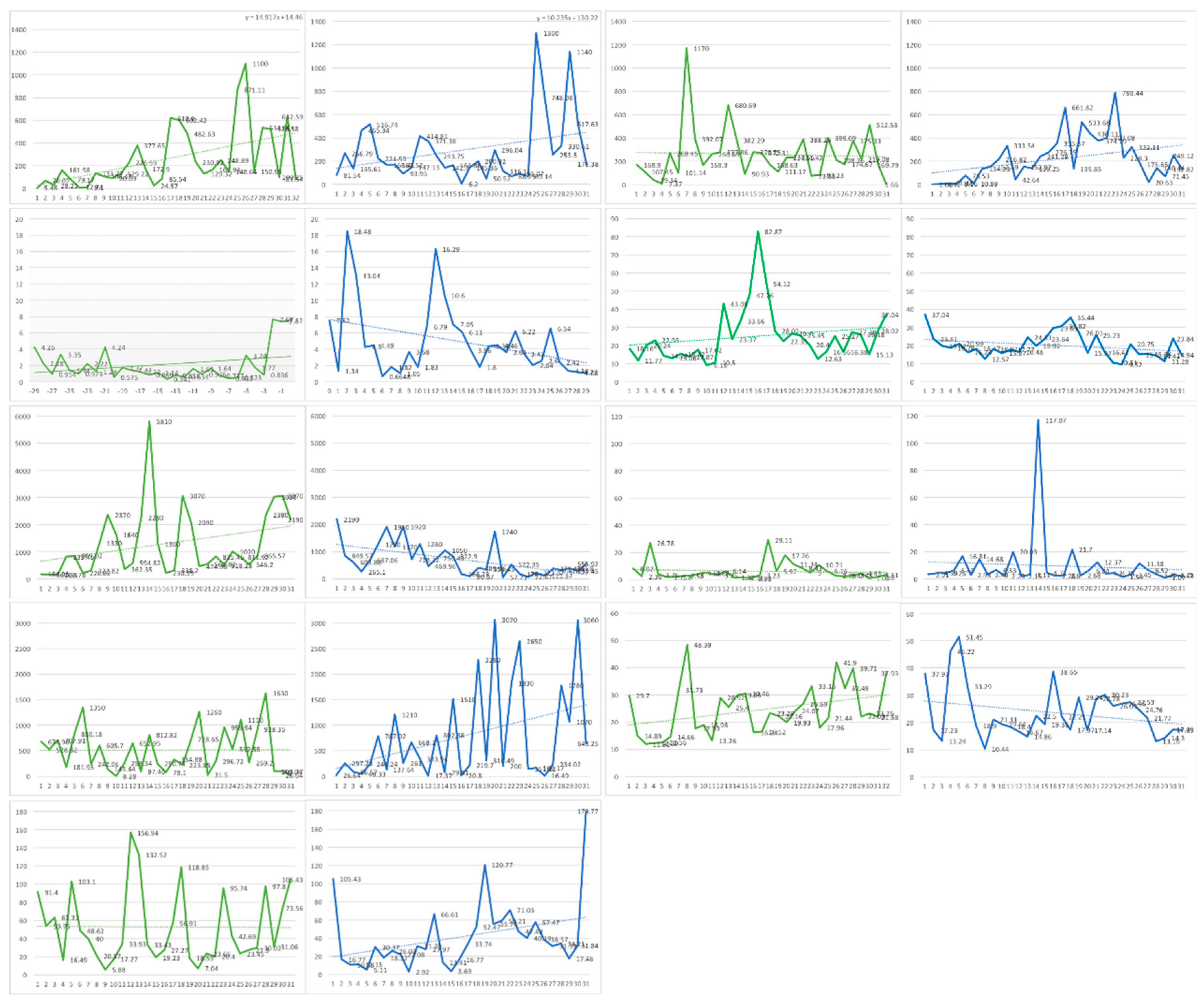
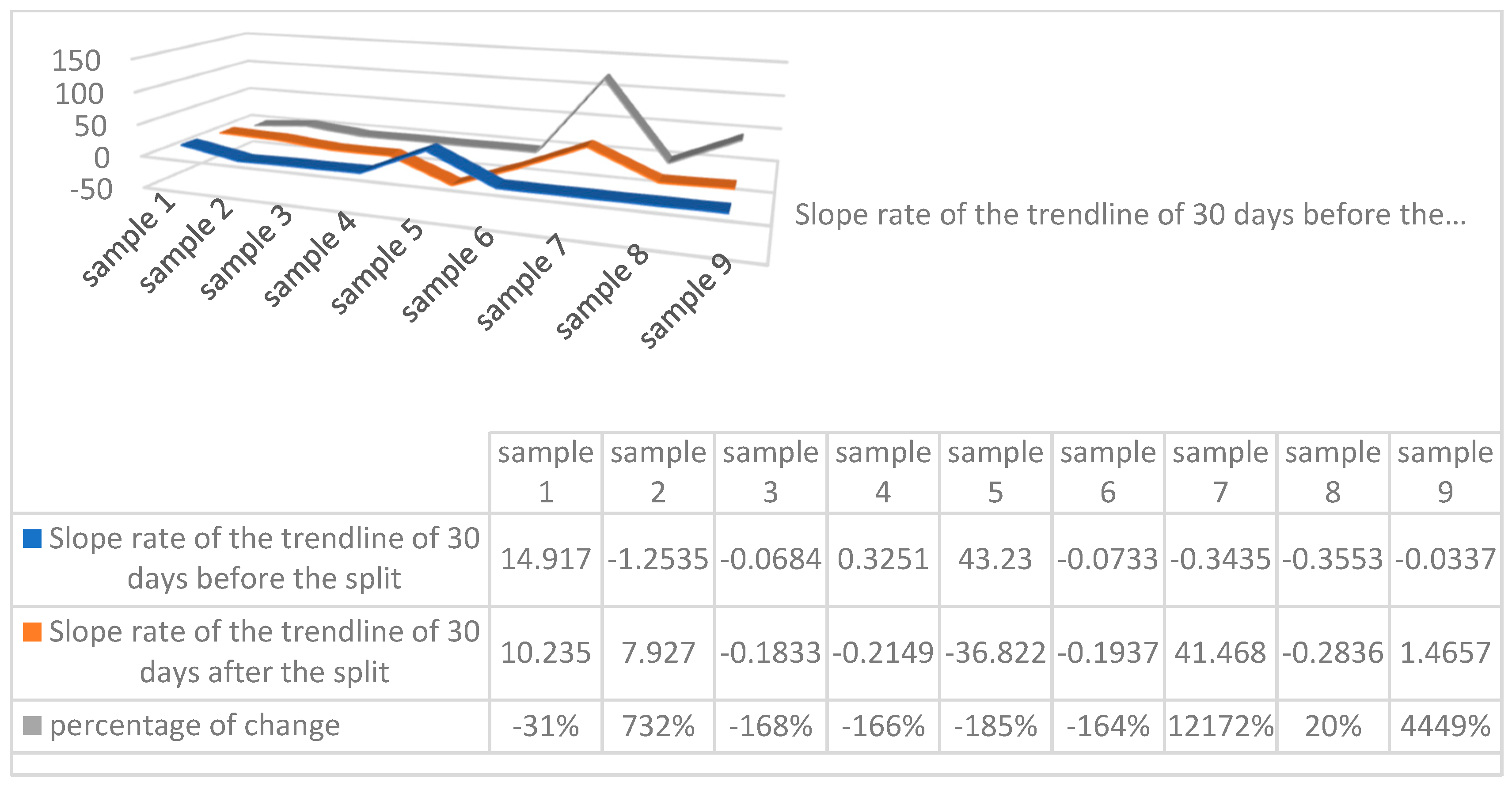
5.3. Hypothesis 3
6. Conclusions
- Stock splits affect the market and slightly enhance the trading volume in the short term.
- Stock splits increase the shareholder base for the firm.
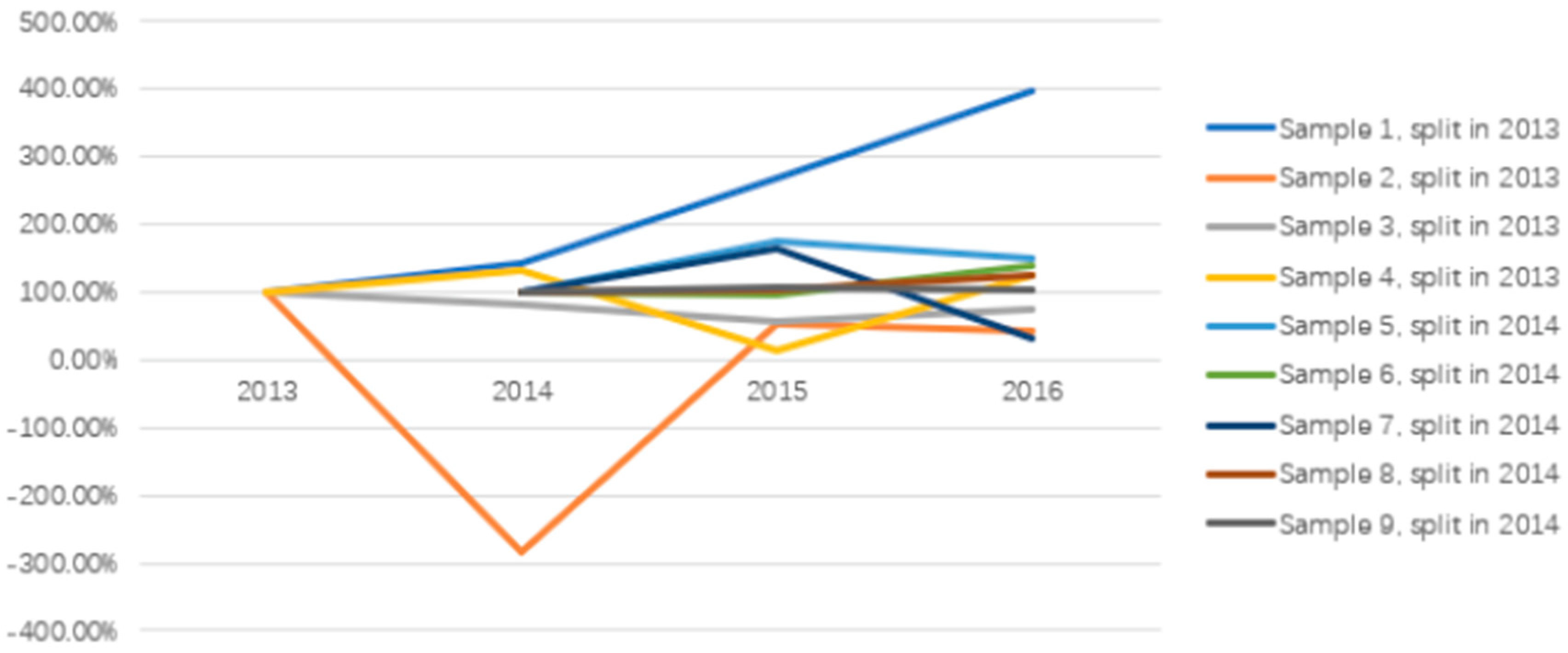
- Most of the firms are mispriced in the split year; stock split announcements reduce the level of information asymmetries.
- Investors readjust their beliefs toward the firm, but (unfortunately?) most of the investors still hold an inexact “fundamental image’’ of the firm.
- Split shares have a positive effect on the liquidity for the market.
Author Contributions
Funding
Institutional Review Board Statement
Informed Consent Statement
Data Availability Statement
Acknowledgments
Conflicts of Interest
References
- Afdhal, Muhammad, Arung Gihna Mayapada, and Sudirman Septian. 2022. Do the COVID-19 Pandemic Affect Abnormal Returns of Stocks in Indonesia? Academy of Entrepreneurship Journal 28: 1–8. [Google Scholar]
- Ausloos, Marcel, and Kristinka Ivanova. 2003. Dynamical Model and Nonextensive Statistical Mechanics of a Market Index on Large Time Windows. Physical Review E 68: 046122. [Google Scholar] [CrossRef] [PubMed] [Green Version]
- Baker, H. Kent, and Gary E. Powell. 1993. The Effect of Stock Splits on the Ownership Mix of a Firm. Review of Financial Economics 3: 70–88. [Google Scholar]
- Baker, H. Kent, and Patricia L. Gallagher. 1980. Management’s View of Stock Split. Financial Management 9: 73–77. [Google Scholar] [CrossRef]
- Barker, C. Austin. 1956. Effective Stock Splits. Harvard Business Review 31: 101–106. [Google Scholar]
- Brennan, Michael J., and Thomas E. Copeland. 1988. Stock Splits, Stock Prices, and Transactions Costs. Journal of Financial Economics 22: 83–101. [Google Scholar] [CrossRef]
- Burnwal, Anshu, and Debdas Rak. 2018. Liquidity and Signalling Aspects of Stock Split: A Study with Reference to Select Indian Companies. International Journal of Research in Management and Social Science 6: 5–24. [Google Scholar]
- Copeland, Thomas. E. 1979. Liquidity Changes Following Stock Splits. American Finance Association 31: 115–141. [Google Scholar] [CrossRef]
- Cornell Law School. n.d. 17 CFR 229.201—(Item 201) Market Price of and Dividends on the Registrant’s Common Equity and Related Stockholder Matters. Cornell Legal Information Institute. Available online: https://www.law.cornell.edu/cfr/text/17/229.201 (accessed on 10 April 2018).
- Dhesi, Gurjeet, and Marcel Ausloos. 2016. Modelling and Measuring the Irrational Behaviour of Agents in Financial Markets: Discovering the Psychological Soliton. Chaos, Solitons & Fractals 88: 119–125. [Google Scholar]
- Easley, David, Maureen O’hara, and Gideon Saar. 2001. How Stock Splits Affect Trading: A Microstructure Approach. The Journal of Financial and Quantitative Analysis 36: 25–51. [Google Scholar] [CrossRef]
- Ferreira, Paulo, and Andreia Dionísio. 2016. How Long is the Memory of the US Stock Market? Physica A: Statistical Mechanics and its Applications 451: 502–506. [Google Scholar] [CrossRef]
- GOV.UK. n.d. Make Changes to Your Private Limited Company. Available online: https://www.gov.uk/make-changes-to-your-limited-company/get-agreement-from-your-company (accessed on 15 February 2018).
- Grinblatt, Mark S., Ronald W. Masulis, and Sheridan Titman. 1984. The Valuation Effects of Stock Splits and Stock Dividends. Journal of Financial Economics 13: 461–490. [Google Scholar] [CrossRef] [Green Version]
- Guo, Fang, Kaiguo Zhou, and Jinghan Cai. 2008. Stock Splits, Liquidity, and Information Asymmetry. An Empirical Study on Tokyo Stock Exchange. Journal of the Japanese and International Economies 22: 417–438. [Google Scholar] [CrossRef]
- Harjoto, Maretno A., Dongshin Kim, Indrarini Laksmana, and Richard C. Walton. 2019. Corporate Social Responsibility and Stock Split. Review of Quantitative Finance and Accounting 53: 575–600. [Google Scholar] [CrossRef]
- Ikenberry, David L., Graeme Rankine, and Earl K. Stice. 1996. What do Stock Splits Really Signal? Journal of Financial and Quantitative Analysis 31: 357–375. [Google Scholar] [CrossRef]
- Karim, Mohammad A., and Sayan Sarkar. 2016. Do Stock Splits Signal Undervaluation? Journal of Behavioral and Experimental Finance 9: 119–124. [Google Scholar] [CrossRef]
- Lakonishok, Josef, and Baruch Lev. 1987. Stock Splits and Stock Dividends: Why, Who, and When. The Journal of Finance 42: 913–932. [Google Scholar] [CrossRef]
- Lamoureux, Christopher G., and Percy Poon. 1987. The Market Reaction to Stock Splits. The Journal of Finance 42: 1347–1370. [Google Scholar] [CrossRef]
- Lo, Andrew W., and Jiang Wang. 2000. Trading Volume: Definitions, Data Analysis, and Implications of Portfolio Theory. The Review of Financial Studies 13: 257–300. [Google Scholar] [CrossRef] [Green Version]
- McNichols, Maureen, and Ajay Dravid. 1990. Stock Dividends, Stock Splits, and Signaling. The Journal of Finance 45: 857–879. [Google Scholar] [CrossRef]
- Miller, Merton H., and Franco Modigliani. 1961. Dividend Policy, Growth, and the Valuation of Shares. The University of Chicago Press Journals 34: 411–433. [Google Scholar] [CrossRef]
- Mohr, Lois A., and Deborah J. Webb. 2005. The Effects of Corporate Social Responsibility and Price on Consumer Responses. The Journal of Consumer Affairs 39: 121–147. [Google Scholar] [CrossRef]
- Popescu, Cristina Raluca Gh, and Gheorghe N. Popescu. 2019. An Exploratory Study Based on a Questionnaire Concerning Green and Sustainable Finance, Corporate Social Responsibility, and Performance: Evidence From the Romanian Business Environment. Journal of Risk and Financial Management 12: 162. [Google Scholar] [CrossRef] [Green Version]
- Romito, Stefano, and Clodia Vurro. 2021. Non-Financial Disclosure and Information Asymmetry: A Stakeholder View on US Listed Firms. Corporate Social Responsibility and Environmental Management 28: 595–605. [Google Scholar] [CrossRef]
- U.S. Securities and Exchange Commission. 2016. Annual Report Pursuant to Section 13 or 15(D) of the Securities Exchange Act of 1934. July 31. Available online: https://www.sec.gov/divisions/corpfin/forms/exchange.shtml (accessed on 10 April 2018).
- Williams, John Burr. 1997. The Theory of Investment Value. Fraser Publishing: Burlington and Cambridge: Harvard University Press. First published 1938. [Google Scholar]
- Yagüe, José, J. Carlos Gómez-Sala, and Francisco Poveda-Fuentes. 2009. Stock Split Size, Signaling and Earnings Management: Evidence from the Spanish Market. Global Finance Journal 20: 31–47. [Google Scholar] [CrossRef]


| #1 | #2 | #3 | #4 | #5 | #6 | #7 | #8 | #9 |
|---|---|---|---|---|---|---|---|---|
| 1.25 | 1.1 | 1.015 | 1.068 | 1.569 | 2 | 1.333 | 1.011 | 4.899 |
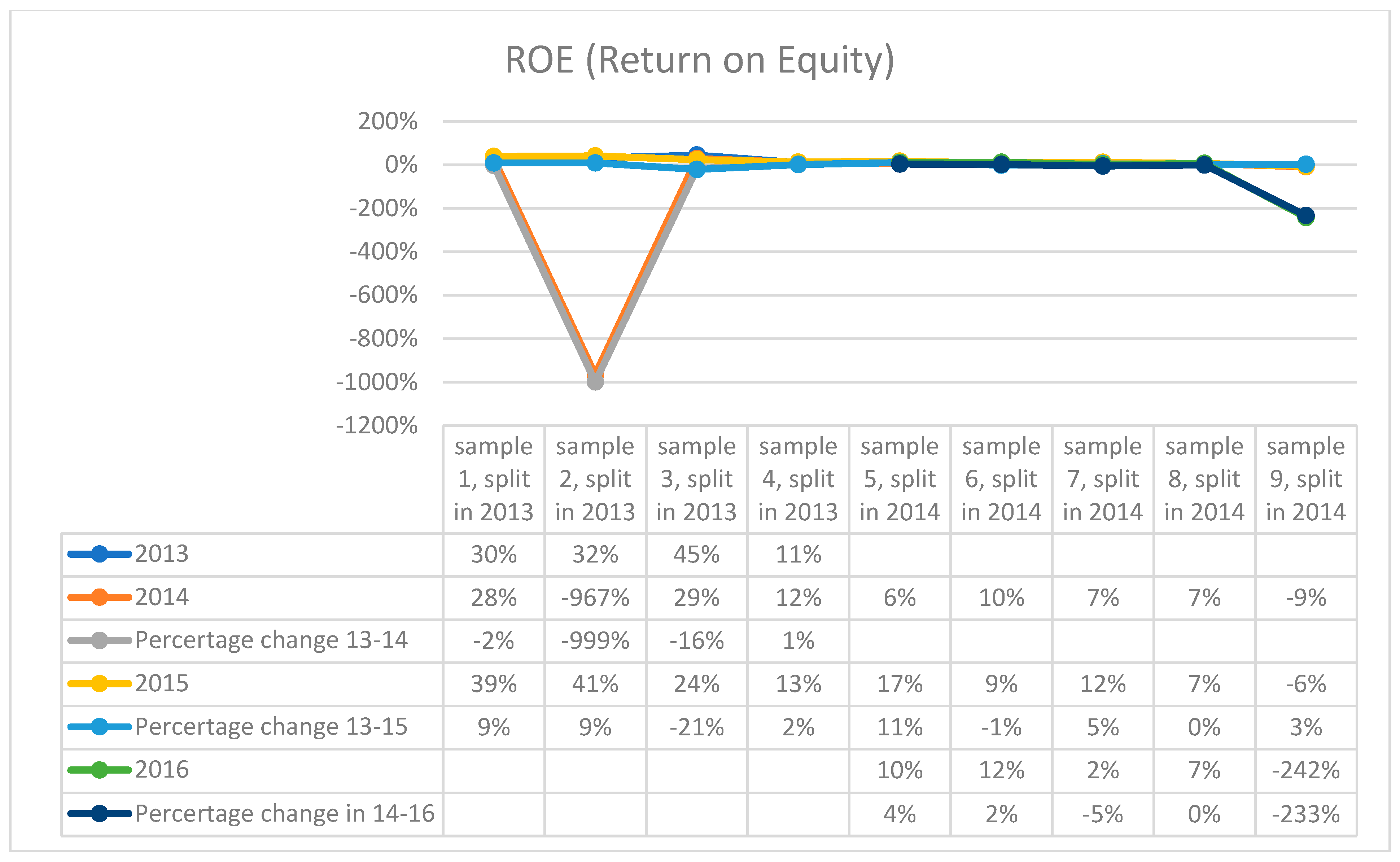
| % Change in Net Profit | 2013 | 2014 | 2015 | 2016 | Total Diff. |
|---|---|---|---|---|---|
| #1(2013) | 100 | 143.94 | 268.58 | 399.29 | 299.29 |
| #2(2013) | 100 | −282.94 | 54.89 | 40.92 | −59.08 |
| #3(2013) | 100 | 80.65 | 58.17 | 73.96 | −26.04 |
| #4(2013) | 100 | 130.54 | 15.40 | 126.35 | 26.35 |
| #5(2014) | 100 | 176.97 | 150.26 | 50.26 | |
| #6(2014) | 100 | 96.48 | 140.17 | 40.17 | |
| #7(2014) | 100 | 164.58 | 31.54 | −68.46 | |
| #8(2014) | 100 | 104.01 | 124.48 | 24.48 | |
| #9(2014) | 100 | 107.34 | 103.91 | 3.91 |
| % Increase | Sample 1 | Sample 4 | Sample 5 | Sample 6 | Sample 8 |
|---|---|---|---|---|---|
| in stock price | 165.5% | 26.27% | 53.07% | 16.03% | 22.06% |
| in the the net profit | 299.29% | 26.35% | 50.26% | 40.17% | 24.48% |
| in the return on equity | 9% | 2% | 4% | 2% | 0% |
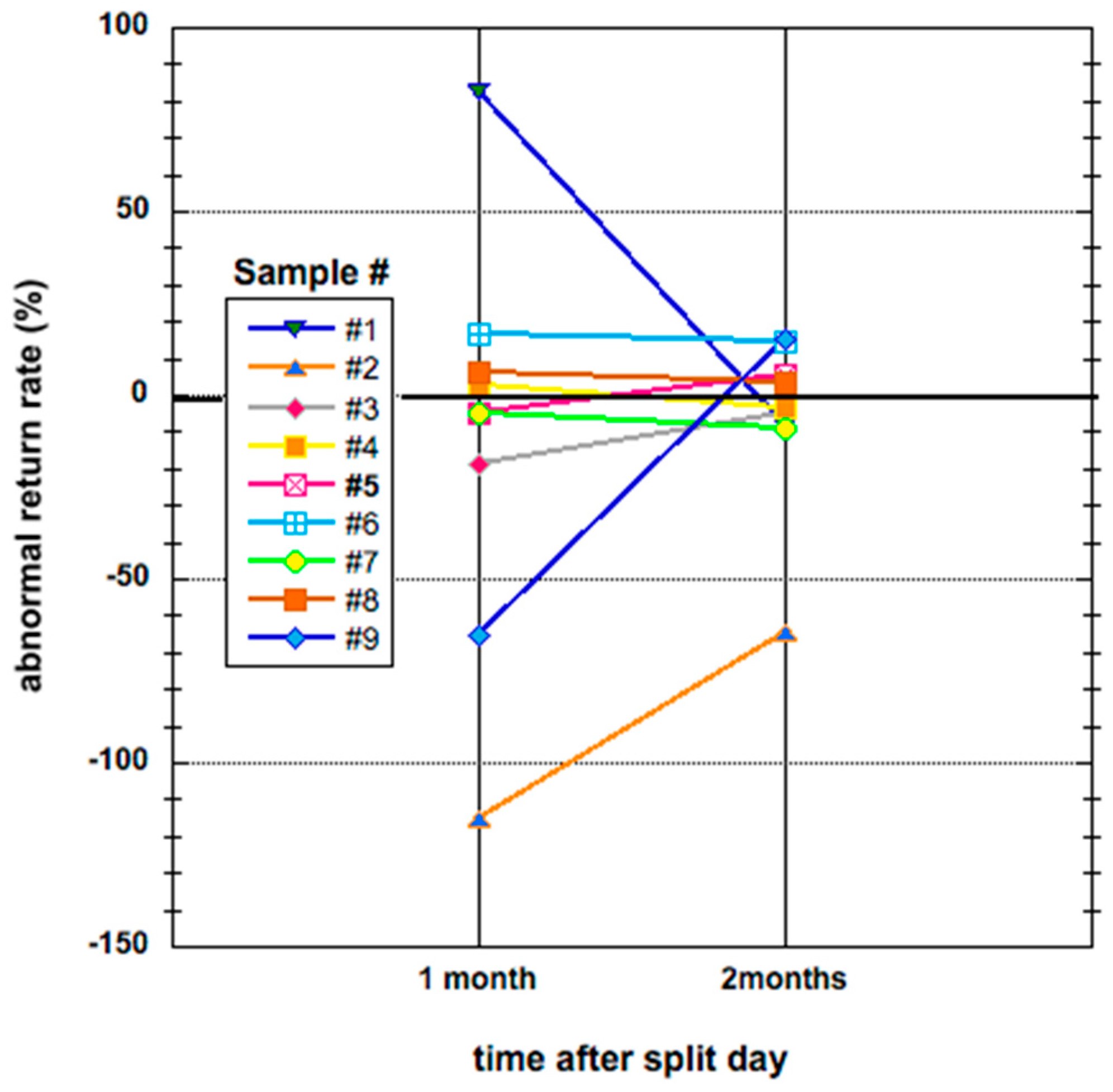
| Sample | #1 | #2 | #3 | #4 | #5 | #6 | #7 | #8 | #9 |
|---|---|---|---|---|---|---|---|---|---|
| % Abnormal return rate after | |||||||||
| 1 month | 82.66 | 115.09 | −18.71 | 2.56 | −4.55 | 16.56 | −4.81 | 6.01 | −65.38 |
| 2 months | −8.55 | −64.92 | −4.68 | −3.19 | 5.54 | 14.65 | −9.02 | 3.36 | 15.38 |
| Sample 1 | Sample 2 | Sample 3 | Sample 4 | Sample 5 | Sample 6 | Sample 7 | Sample 8 | Sample 9 |
|---|---|---|---|---|---|---|---|---|
| −0.09066 | 0.04821 | 0.01182 | −0.01784 | −0.16377 | 0.01110 | 0.08801 | 0.04164 | −0.00246 |
Disclaimer/Publisher’s Note: The statements, opinions and data contained in all publications are solely those of the individual author(s) and contributor(s) and not of MDPI and/or the editor(s). MDPI and/or the editor(s) disclaim responsibility for any injury to people or property resulting from any ideas, methods, instructions or products referred to in the content. |
© 2023 by the authors. Licensee MDPI, Basel, Switzerland. This article is an open access article distributed under the terms and conditions of the Creative Commons Attribution (CC BY) license (https://creativecommons.org/licenses/by/4.0/).
Share and Cite
Chen, J.; Ausloos, M. A Study about Who Is Interested in Stock Splitting and Why: Considering Companies, Shareholders, or Managers. J. Risk Financial Manag. 2023, 16, 68. https://doi.org/10.3390/jrfm16020068
Chen J, Ausloos M. A Study about Who Is Interested in Stock Splitting and Why: Considering Companies, Shareholders, or Managers. Journal of Risk and Financial Management. 2023; 16(2):68. https://doi.org/10.3390/jrfm16020068
Chicago/Turabian StyleChen, Jiaquan, and Marcel Ausloos. 2023. "A Study about Who Is Interested in Stock Splitting and Why: Considering Companies, Shareholders, or Managers" Journal of Risk and Financial Management 16, no. 2: 68. https://doi.org/10.3390/jrfm16020068