An Application of Portfolio Mean-Variance and Semi-Variance Optimization Techniques: A Case of Fiji

Abstract

In this paper, we apply the Markowitz portfolio optimization technique based on mean-variance and semi-variance as measures of risk on stocks listed on the South Pacific Stock Exchange, Fiji. We document key market characteristics and consider monthly returns data from SEP-2019 to FEB-2022 (T = 30) of 17/19 listed companies on the stock exchange to construct various portfolios like 1/N (naïve), maximum return, and market and minimum-variance with and without short-selling constraints. Additionally, we compute each stock’s beta using the market capitalization-weighted stock price index data. We note that well-diversified portfolios (market portfolio and minimum-variance portfolio) with short-selling constraints have relatively higher expected returns with lower risk. Moreover, well-diversified portfolios perform better than the naïve and maximum portfolios in terms of risk. Moreover, we find that both the mean-variance and the semi-variance measures of risk yields a unique market portfolio in terms of expected returns, although the latter has a lower standard deviation and a higher Sharpe ratio. However, for the minimum-variance portfolios and market portfolios without short selling, we find relatively higher returns and risks using the mean-variance than the semi-variance approach. The low beta of individual stock indicates the low sensitivity of its price to the movement of the market index. The study is an initial attempt to provide potential investors with some practical strategies and tools in developing a diversified portfolio. Since not all the portfolios based on mean-variance and the semi-variance analyses are unique, additional methods of investment analysis and portfolio construction are recommended. Subsequently, for investment decisions, our analysis can be complemented with additional measures of risk and an in-depth financial statement/company performance analysis.

1. Introduction

It is well-known in economic science (Levine 2005) that well-functioning financial markets contribute significantly to economic growth. A part of the financial market is represented by the stock exchange market. A problem with investors living in a country with fixed exchange rates and capital controls, such as Fiji, is that it is difficult to invest abroad. Given this restriction, investors can choose to deposit their savings and monetary wealth into bank accounts or they can buy company shares via stockbrokers at the stock exchange. Therefore, it is important that investors fully understand the stock market. In this paper, we consider the data of companies listed on the South Pacific Stock Exchange (SPX) as a case to construct a market and minimum variance portfolio based on the Markowitz portfolio optimization technique (Markowitz 1952, 1959, 1990, 1991; Rubinstein 2002; Sharpe 1964, 1971; Konno and Yamazaki 1991; Baumann and Trautmann 2013; c.f. Chavalle and Chavez-Bedoya 2019; Sun et al. 2021).

In general, buying stocks means that the investor becomes a shareholder of the respective company and the shares give the shareholder the right to vote on matters concerning their interests. The shareholders of firms listed on the stock exchange are legally much better protected than the shareholders of unlisted firms. This is because a stock exchange is an institution that regulates the market for stocks so that the investors are protected against fraudulent and unfair trade practices. The main advantage of investing in stocks is that the returns can be influenced by the portfolio choice, which usually increases the profitability of investments. However, because the stock prices can be susceptible to greater downside risk than the upside gains, this can result in the investor losing part of her investment, or, in the worst situations, the whole investment.

In general, a portfolio refers to the number of stocks, bonds, or other financial or real assets owned by an individual, a group of people, or a company with the aim of making profits. Any rational investor will choose the portfolio from the efficient frontier because it promises the optimal combination of the risk and return, where risk is measured by the standard deviation and return is the average percentage change of the stock prices. To compensate for the risk undertaken, the investor has to require a risk premium, where the risk premium is defined as the expected return that exceeds the risk-free rate of return. Accordingly, the bigger the risk, the higher the risk premium needed by the investors to compensate for the risk undertaken.

Regarding risk in the financial market, we can differentiate between systematic risk and unsystematic risk. Systematic, market, or macroeconomic risk refers to the risk that affects the whole market or a large number of assets to varying degrees due to inflation, interest rates, unemployment rates, currency exchange rates, and natural disasters. Unfortunately, systematic risks cannot be eliminated by the portfolio choice. On the other hand, unsystematic, specific, or idiosyncratic risk occurs at the micro- or firm level, which can affect a single asset or a small group of assets. Factors influencing unsystematic risk includes credit ratings, news coverage of the corporation, financial and management decisions, the entrance of a new competitor in the marketplace, a change in market regulation, product recalls, and so on. In contrast to systematic risks, unsystematic risks can be reduced substantially through the diversification of assets within a portfolio.

For our purpose, we use Markowitz’s (1952, 1959) approaches to construct minimum-variance and market portfolios. In the original Markowitz’s model (Markowitz 1952) risk is measured by the standard deviation or variance. The original Markowitz model is a quadratic programming problem. Following Sharpe (1971), attempts have been made to linearize the portfolio optimization problem. The risk component of Modern Portfolio Theory can be mitigated through the concept of diversification. Diversification requires carefully selecting a weighted collection of investment assets that collectively exhibit lower risk characteristics than any single asset or asset class. As noted by Rubinstein (2002, p. 1043) in praise of Markowitz’s models, “… the decision to hold a security should not be made simply by comparing its expected return and variance to others, …the decision to hold any security would depend on what other securities the investor wants to hold”.

In this study, the mean-variance and semi-variance approaches of Markowitz are suitable for consideration because, ideally, these approaches are both practical and can be easily implemented to optimize small-scale portfolios (c.f. Konno and Yamazaki 1991). The key assumptions of the Markowitz technique are that: (i) investors are rational, i.e., they seek to maximize returns while minimizing risk; (ii) investors will accept increased risk if they are compensated with higher expected returns; (iii) investors receive or have all the necessary information regarding their investment decisions in a timely manner; (iv) investors can borrow or lend an unlimited amount of capital at a risk-free rate of interest. In challenging these assumptions and noting that the approaches may not be suitable for large-scale portfolios, Konno and Yamazaki (1991, p. 521) highlight that “Markowitz’s model should be viewed as an approximation into the more complicated optimization problem facing an investor”, whilst presenting alternative methods of portfolio construction for large-scale portfolios.

Indeed, the portfolio optimization technique has advanced to a great degree (Baumann and Trautmann 2013; Turcas et al. 2017; Chavalle and Chavez-Bedoya 2019; Becker et al. 2015). In this study, we apply the basic mean-variance and semi-variance analyses (Markowitz 1952, 1959) using the data of companies listed on the South Pacific Stock Exchange (SPX) in Fiji. It must be noted that Fiji’s stock market is less developed, less sophisticated, and relatively small, with 19 companies listed on the Exchange. Therefore, to construct small-scale portfolios, the analysis can easily consider all plausible securities. Currently, the total stock market capitalization is just over FJD 3 billion (c.f. Saliya 2020). The rest of the paper is outlined as follows. Section 2 outlines the basic methodology/framework for analysis. Section 3 describes data and presents a qualitative data analysis on companies listed on SPX. In Section 4, we construct mean-variance and semi-variance portfolios (without and with short selling), minimum-variance portfolios (without and with short selling), and estimate each stock’s beta. In Section 5, the conclusion follows.

2. Materials and Methods

A portfolio constructed from N different securities is given by $\mathit{\omega }=\left({\omega }_1,\dots ,{\omega }_n\right),$ where ${\displaystyle \sum }_{i=1}^n{\omega }_i=1$, and $\mathbf{1}=\left(1,\dots ,1\right)$, is used for an nx1 unit vector. The constraint can be written as ${\mathit{\omega }}^{\mathit{T}}\mathbf{1}=1$. The attainable set $A$ consists of all possible portfolios with weights $\omega$, such that $A=\left\{\mathit{\omega }:{\mathit{\omega }}^{\mathit{T}}\mathbf{1}=1\right\}$. With the assumption of short-selling constraints, ${\omega }_i\ge 0\forall i$, and with short selling, ${\omega }_i\le 1$. The mean-variance (MV) model is given by:

$$Max. {\displaystyle \sum }_{i=1}^N{\overline{r}}_i{\omega }_i.$$

$$s.t. \{\begin{array}{}\mathrm{(1)}& {\displaystyle {\displaystyle \sum }_{i=1}^N}{\displaystyle \sum }_{j=1}^N{\sigma }_{ij}{\omega }_i{\omega }_j\le \delta \mathrm{(2)}& {\displaystyle \sum }_{i=1}^N{\omega }_i=1\end{array}$$

where $N$ is the number of stocks as stated earlier, ${\sigma }_{ij}$ is the covariance between return of stock $i$ and return of stock $j$, ${\overline{r}}_i$ is the expected return of stock $i$, $\delta$ is the maximal risk level, and ${\omega }_i$ is the weight of stock $i$ in the portfolio. Constraints (1) and (2) represent the risk constraint and budget constraints, respectively. The random return $r_t$ of each stock at a given time $t$ is given by $r_t=\ln \left(\frac{P_{t+1}}{P_t}\right)$, where $P_t$ and $P_{t+1}$ are the prices of a stock in period t and period t + 1, respectively. The covariance between returns is denoted by ${\sigma }_{ij}$.

Moreover, the portfolio with the smallest variance in the attainable set has weights, ${\mathit{\omega }}_{\mathit{m}\mathit{i}\mathit{n}}=\frac{{\Sigma }^{\mathbf{-}\mathbf{1}}}{{\mathbf{1}}^{\mathit{T}}{\Sigma }^{\mathbf{-}\mathbf{1}}\mathbf{1}}$, where ${\Sigma }^{\mathbf{-}\mathbf{1}}$ is the inverse covariance of returns. Finally, a portfolio’s expected return ${\mathit{\mu }}_{\mathit{\omega }}$ and variance ${\mathit{\sigma }}_{\mathit{\omega }}^{\mathbf{2}}$ is given by ${\mathit{\mu }}_{\mathit{\omega }}={\mathit{\omega }}^{\mathit{T}}\mathit{\mu }$ and ${\mathit{\sigma }}_{\mathit{\omega }}^{\mathbf{2}}={\mathit{\omega }}^{\mathit{T}}\Sigma \mathit{\omega }$, respectively, where $\Sigma$ is the covariance matrix.

It must be noted that variance (of returns) as a risk measurement equally penalizes gains and losses in the mean-variance analysis. To account for the downside risk only, an alternative measure of risk proposed by Markowitz (1959) is the semi-variance measure. Hence, following Markowitz (1959), the downside risk is defined as: $D_{risk}=\frac{1}{T}{\displaystyle \sum }_{i=1}^n{\left[\min \left(R_i-B,0\right)\right]}^2$, where $B$ is the benchmark return selected by the investor. The benchmark can be set either to zero or to the average return. For our purpose, we define B as the non-negative return such that: $B=\max \left(\overline{R},0\right)$ where $\overline{R}$ is the average return of the stock i. Semi-covariance can be defined as: ${\Sigma }_{\mathit{D}\mathit{R}}=\frac{\mathbf{1}}{\mathit{T}}{\displaystyle \sum }_{\mathit{i}\mathbf{=}\mathbf{1}}^{\mathit{N}}\left[\min \left(R_{i,t}-B,0\right)\times \min \left(R_{j,t}-B,0\right)\right]$, where T is the number of observations, and $R_{i,t}$ is the return of asset i. The Sharpe ratio is computed as: $SR=\frac{\mu -r_f}{\sigma }$, where $\mu$, $r_f$, and $\sigma$ are portfolio mean, risk-free rate (in our case it is 1.5%), and portfolio standard deviation, respectively. Maximizing SR (and adjusted SR in the case of semi-variance analysis) will yield the market portfolio. A market portfolio refers to the optimal portfolio of risky assets. If the risk free rate, $r_f$ is smaller than the expected return of the minimum variance portfolio; then, the market portfolio exists and is given by: ${\mathit{\omega }}_{\mathit{m}\mathit{k}\mathit{t}}=\frac{{\Sigma }^{\mathbf{-}\mathbf{1}}\left(\mathit{\mu }\mathbf{-}{\mathit{r}}_{\mathit{f}}\mathbf{1}\right)}{{\mathbf{1}}^{\mathit{T}}{\Sigma }^{\mathbf{-}\mathit{1}}\left(\mathit{\mu }\mathbf{-}{\mathit{r}}_{\mathit{f}}\mathbf{1}\right)}$, where ${\Sigma }^{\mathbf{-}\mathbf{1}}$ is the inverse covariance matrix, $\mu$ is the vector of expected returns, and $\mathbf{1}$ is a vector 1 s. In addition, we estimate the asset’s beta using the formula: ${\beta }_i=\frac{COV\left({\mu }_i,{\mu }_m\right)}{Var\left({\mu }_i\right)}$, where ${\mu }_i$ refers to individual stock returns, and, for our purpose, we use the changes in market capitalization-weighted price index as a proxy for ${\mu }_m$.

3. Data

As noted earlier, there are 19 companies listed on the SPX (

Table 1. Listed Companies on SPX.

Symbol	Company	Date Listed	Sector
APP	Atlantic & Pacific Packaging Company Limited	17 August 1998	Manufacturing and Wholesale
ATH	Amalgamated Telecom Holdings Limited	18 April 2002	Telecommunications and Media
BCN	BSP Convertible Notes Limited	11 May 2010	Bking
CFL	Communications Fiji Limited	20 December 2001	Telecommunications and Media
FBL	Free Bird Institute Limited	2 February 2017	Education
FHL	Fijian Holdings Limited	20 January 1997	Investment
FIL	FijiCare Insurance Limited	7 December 2000	Insurance
FMF	Flour Mills of Fiji (FMF) Foods Limited	25 July 1979	Manufacturing and Wholesale
FTV	Fiji Television Limited	24 April 1997	Telecommunications and Media
KGF	Kinetic Growth Fund Limited	16 December 2004	Investment
KFL	Kontiki Finance Limited	4 July 2018	Finance
PBP	Pleass Global Limited	4 February 2009	Manufacturing and Wholesale
PGI	Pacific Green Industries Fiji Limited	5 June 2001	Manufacturing and Wholesale
PDM	Port Denarau Marina Limited	14 August 2019	Tourism
RBG	RB Patel Group Limited	17 January 2001	Retail
RCF	The Rice Company of Fiji Limited	20 January 1997	Manufacturing and Wholesale
TTS	Toyota Tsusho South Sea Limited	7 June 1979	Automotive
VBH	VB Holdings Limited	1 November 2001	Automotive
VIL	Vision Investment Limited	29 February 2016	Investment

Source: Data on respective company’s profile from SPX website (accessed on 3 March 2022).

). In terms of sectoral distribution, five companies (APP, FMF, PBP, PGI and RCF) belong to Manufacturing and Wholesale, three belong to Telecommunications and Media (ATH, CFL and FTV), two (TTS and VBH) to Automotive, three (FHL, KGF and VIL) to Investment, one (BCN) to Banking, one (FBL) to Education, one to (FIL) Insurance, one (KFL) to Finance, one (PDM) to Tourism, and one (RBG) to Retail.

4. Qualitative Data Analysis

Table 2. SPX Daily Quotes.

Code	Current Market Price (F$)	Closing Quotes		Earnings Per Share (FJ Cents)	Price Earnings Ratio (Times)	Current Yield (%) (Dividend/Interest)	Market Capitalization (F$, Million)	% of Market Cap.
		Buy (F$)	Sell (F$)
APP	3.20	2.91	3.20	26.81	11.93	1.72	25.60	0.82%
ATH	1.78	1.75	1.83	8.64	20.59	1.12	851.89	27.36%
CFL	7.00	6.30	7.00	23.17	30.21	1.14	24.91	0.80%
FBL	4.02	2.93	4.02	29.91	13.44	18.66	9.55	0.31%
FIL	7.60	6.60	7.18	18.56	40.96	0.66	65.42	2.10%
FMF	1.99	-	1.99	6.13	32.46	1.51	298.50	9.59%
FTV	4.50	-	4.50	−22.79	−19.74	0.00	46.35	1.49%
KFL	1.00	0.85	1.09	4.59	21.76	3.00	92.88	2.98%
KGF	1.12	0.84	1.12	−0.99	−112.85	0.00	4.28	0.14%
PBP	3.20	2.75	3.15	15.51	20.63	1.25	21.88	0.70%
PDM	2.14	1.80	2.14	−14.56	−14.70	0.00	85.60	2.75%
PGI	1.08	-	-	3.82	28.26	0.00	8.23	0.26%
RBG	3.38	2.80	3.38	5.71	59.15	0.95	507.00	16.28%
RCF	11.20	-	11.00	35.70	31.37	3.13	67.20	2.16%
TTS	19.25	15.10	19.24	39.81	48.36	1.04	270.12	8.67%
VBH	7.50	-	7.50	65.49	11.45	0.93	16.03	0.51%
VIL	4.15	-	4.15	6.76	61.41	1.20	430.64	13.83%
FHL	0.63	0.45	0.63	−5.78	−10.91	0.00	191.93	6.16%
BCN	31.28	31.38	31.50	84.98	36.81	2.62	95.87	3.08%

Source: SPX Website—closing quotes as of 24 February 2022.

(below) shows the current market prices (FJ$), earnings per share (in FJ cents), price-earnings ratio, market capitalization, and size of each company relative to the market capitalization. The companies with a relatively larger market cap (>5%) are ATH (27.4%), RBG (16.28%), VIL (13.8%), FMF (9.6%), and TTS (8.7%), among others, and those with the smallest cap (<1%) are KGF (0.1%), PGI (0.3%), FBL (0.3%), VBH (0.5%), PBP (0.7%), and CFL (0.8%)

According to SPX (2020b), in the year 2020, there were 260 new investors (security holders) in the SPX market. The majority of the investors were individuals (75%), followed by joint/family (10%), Trusts and Institutions (11%), and others (4%). Moreover, among the new investors, 28% were from the private sector, followed by 22% from the ‘others’ category, which included minors, institutions, and self-employed individuals. A total of 19% were from the public sector, 10% were retirees, 9% were students, 7% were farmers, and 5% were domestic workers. In terms of age group, 37% of the investors were in the age range 36–55 years, followed by 25% in the age range 26–35 years, 19% over 55 years, 14% in the range 18–25 years, and the remainder were below 18 years. In terms of the geographic distribution of new investors, most were from Central/Eastern (78%), followed by Western (17%), Northern (2%), and non-residents (3%).

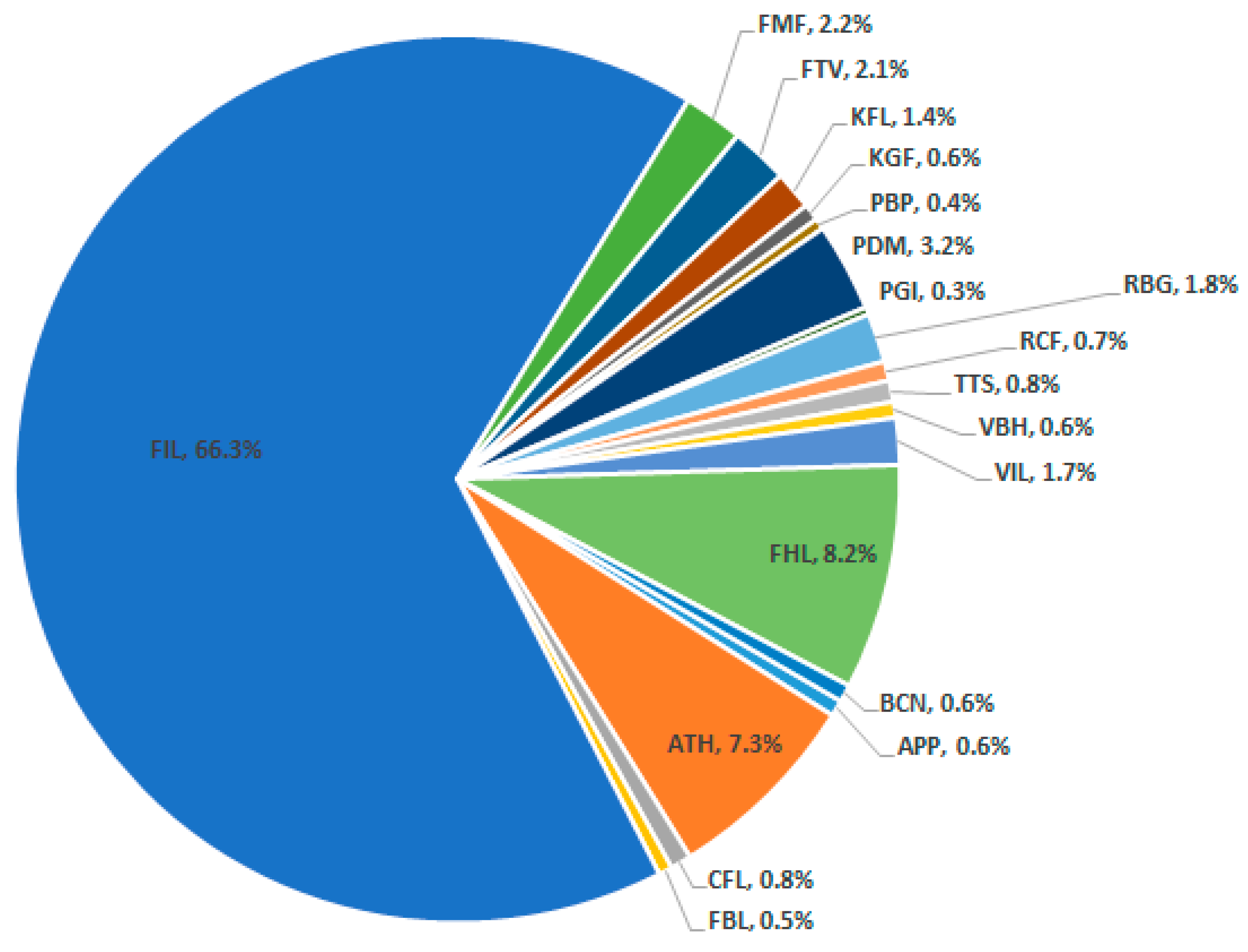
There are total of 20,146 security holders in the stock market (

Table 3. Distribution of Security Holding and Number of Security Holders.

												Number of Resident & Non-Resident Security Holders		Percentage of Public & Non-Public Security Holding
Security	<500	501–5000	5001–10,000	10,001–20,000	20,001–30,000	30,001–40,000	40,001–50,000	50,001–100,000	100,001–1,000,000	>1,000,000	Total	Resident Security Holders	Non-Resident Security Holders	Public	Non—Public
APP	16	71	14	10	3	0	0	3	4	1	122	113	9	26.13%	73.87%
ATH	284	948	126	44	15	6	9	15	7	9	1463	1376	87	10.49%	89.51%
CFL	44	88	7	2	4	2	0	2	4	1	154	136	18	28.82%	71.18%
FBL	65	19	5	2	2	1	1	1	2	1	99	72	27	30.41%	69.60%
FIL	13,275	49	8	7	5	0	0	3	4	1	13,352	13,341	11	22.10%	77.90%
FMF	27	109	67	72	40	17	22	33	44	9	440	349	91	29.25%	70.75%
FTV	207	200	8	4	1	0	0	0	3	2	425	385	40	17.90%	82.10%
KFL	30	79	26	22	13	12	5	21	51	24	283	219	64	55.94%	44.06%
KGF	3	72	15	14	5	3	1	4	6	1	124	112	12	77.93%	22.07%
PBP	17	39	11	5	1	1	0	2	3	2	81	79	2	26.05%	73.95%
PDM	218	326	56	23	3	7	3	7	4	3	650	619	31	29.48%	70.52%
PGI	16	29	0	2	1	1	0	1	3	3	56	47	9	6.38%	93.62%
RBG	41	151	38	34	33	3	20	14	15	9	358	339	19	28.75%	71.25%
RCF	43	76	7	6	3	2	0	1	3	1	142	129	13	17.82%	82.18%
TTS	106	39	4	2	0	1	0	1	1	2	156	91	65	20.32%	79.68%
VBH	44	52	6	4	1	0	3	2	5	0	117	98	19	22.38%	77.62%
VIL	63	169	63	18	6	1	3	3	9	9	344	337	7	19.83%	80.17%
FHL	155	565	321	221	86	51	40	69	128	19	1655	1630	25	31.33%	68.67%
BCN	56	52	2	0	1	2	3	3	5	1	125	122	3	37.86%	62.14%
Total	14,710	3133	784	492	223	110	110	185	301	98	20,146	19,594	552	28.38%	71.62%
% of shareholders	73.0%	15.6%	3.9%	2.4%	1.1%	0.5%	0.5%	0.9%	1.5%	0.5%

Source: SPX (2020a) and authors’ calculations based on data from SPX (2020a).

). About 66% of the security holders own securities of FIL (Figure 1), out of which majority holds (99%) below 500 securities. Overall, about 73% of investors hold fewer than 500 securities across all the securities, and about 0.5% of the investors own more than one million securities (see the last row of Table 3). In terms of investor type, 55% of the security holders are male, 15% are female, 4% are trusts and corporates, and 26% are ‘others’ (

Table 4. Number of Resident and Non-Resident Security Holders by Investor Type and Gender.

Type/Gender	Resident Security Holders	Non-Resident Security Holders
Male	11,463	429
Female	3160	105
Trust	244	13
Corporate	512	71
Others	4726	770
Total	20,105	1388

Source: SPX (2020a).

). In terms of the percent of resident (non-resident) security holders, 57% (31%) are male and 16% (8%) are female investors (Figure 2 and Figure 3). Moreover, in terms of the percentage of security holding by investor type (

Table 5. Percentage of Security Holding by Investor Type.

Security	Individual	Institution/Company	Trust	Joint/Family	Others
APP	4.09%	89.26%	5.62%	0.49%	0.5%
ATH	0.84%	96.55%	2.31%	0.13%	0.2%
CFL	9.64%	74.87%	13.08%	2.27%	0.1%
FBL	12.31%	73.64%	12.64%	1.01%	0.4%
FIL	5.84%	92.38%	0.82%	0.41%	0.6%
FMF	11.47%	86.06%	2.01%	0.45%	0.0%
FTV	3.26%	87.11%	8.79%	0.65%	0.2%
KFL	40.36%	48.06%	5.39%	4.91%	1.3%
KGF	17.49%	79.24%	0.08%	3.10%	0.1%
PBP	55.83%	27.45%	16.35%	0.36%	0.0%
PDM	3.81%	94.77%	0.88%	0.50%	0.0%
PGI	11.56%	70.44%	17.54%	0.47%	0.0%
RBG	6.98%	88.99%	3.30%	0.34%	0.4%
RCF	3.76%	94.30%	1.02%	0.71%	0.2%
TTS	0.44%	99.32%	0.14%	0.10%	0.0%
VBH	61.47%	23.90%	14.39%	0.23%	0.0%
VIL	1.21%	92.96%	2.27%	0.42%	3.1%
FHL	5.55%	79.51%	2.20%	2.49%	10.3%
BCN	4.22%	90.36%	3.83%	0.27%	1.3%

Source: SPX (2020a).

), we note that individual investors make up the largest proportion of securities holders for KFL (40%), PBP (56%), and VBH (61%), whereas for other the securities, company/institution hold a significant percentage of the securities. In terms of geographical spread of the total number of security holders (

Table 6. Percentage of Resident Retail Security Holding by Location, Resident Institutional, and Non-Resident Security Holding.

Security	Total Issued Securities (Millions)	Resident-Individual			Resident-Institutional	Total Resident Security Holding	Total Non-Resident Security Holding
		Central/Eastern	Western	Northern
APP	8.0	20.15%	0.82%	0.03%	78.22%	99.22%	0.79%
ATH	422.1	2.90%	0.36%	0.03%	96.18%	99.47%	0.53%
CFL	3.6	23.24%	0.52%	0.00%	73.84%	97.60%	2.40%
FBL	2.0	1.41%	2.32%	0.00%	15.27%	19.00%	81.00%
FIL	8.6	6.40%	0.15%	0.01%	92.18%	98.73%	1.27%
FMF	150.0	7.94%	2.94%	0.28%	86.03%	97.19%	2.81%
FTV	10.3	2.28%	1.16%	0.13%	95.96%	99.52%	0.48%
KFL	91.5	16.27%	0.92%	0.02%	40.21%	57.42%	42.58%
KGF	3.8	17.70%	1.31%	0.42%	63.54%	82.97%	17.03%
PBP	6.7	55.79%	0.27%	0.00%	43.79%	99.85%	0.15%
PDM	40.0	2.63%	1.18%	0.07%	25.04%	28.92%	71.08%
PGI	7.6	0.82%	0.58%	0.00%	87.98%	89.37%	10.63%
RBG	150.0	6.16%	4.63%	0.11%	88.92%	99.81%	0.19%
RCF	6.0	4.01%	0.76%	0.21%	94.27%	99.26%	0.74%
TTS	14.0	0.43%	0.04%	0.01%	19.61%	20.08%	79.92%
VBH	2.1	65.05%	0.31%	0.09%	21.39%	86.85%	13.15%
VIL	103.8	3.36%	0.58%	0.00%	92.95%	96.89%	3.11%
FHL	304.7	6.77%	0.64%	0.23%	91.93%	99.58%	0.42%
BCN	3.1	4.18%	0.28%	0.01%	95.17%	99.65%	0.35%

Source: SPX (2020a).

), the number of resident-investors are mainly from the Central/Eastern division except for FBL (2.3%). Furthermore, on aggregate, the percentage of non-residential security holdings are very small, except for FBL (81%), KFL (43%), PDM (71%) and TTS (80%). Therefore, the market portfolio and minimum-variance portfolio that we present in the analyses that follow are likely to be based on trading activities that are for the most part driven by companies, males, and investors from the Central/Eastern division. Arguably, a broader participation can influence the risk-return profiles of securities and hence portfolio selection, which at the moment cannot be ascertained due to the low participation of females and individuals from other divisions.

In what follows, we summarize on an annual basis the average share price, the number, the volume, and the total value of trade of each company’s share (

Table 7. Average Share Price Per Year.

Year	APP	ATH	BCN	CFL	FBL	FHL	FIL	FMF	FTV	KGF	KFL	PBP	PGI	PDM	RBG	RCF	TTS	VBH	VIL
2010	$0.77	$0.92	-	$1.76	-	$3.16	$0.63	$0.45	$3.04	$0.47	-	$0.92	-	-	$1.79	-	$1.90	-	-
2011	$0.77	$0.86	$6.19	$1.92	-	$2.87	$0.50	$0.43	$2.59	$0.33	-	$0.91	$2.03	-	$1.95	$2.30	$1.87	$2.98	-
2012	$0.73	$0.77	$6.16	$2.17	-	$2.84	$0.41	$0.40	$2.58	$0.28	-	$0.85	$2.00	-	$2.10	$2.30	$2.20	$2.99	-
2013	$0.70	$0.73	$6.87	$2.60	-	$3.11	$0.56	$0.43	$2.87	$0.29	-	$0.86	$2.00	-	$2.28	$2.30	$2.20	$3.05	-
2014	$0.68	$0.86	$6.95	$3.97	-	$3.37	$0.60	$0.51	$2.90	$0.28	-	$0.94	$2.00	-	$2.63	2.58	$2.95	3.13	-
2015	$0.88	$1.07	$7.12	$4.14	-	$3.95	$0.68	$0.66	$2.36	$0.41	-	$1.07	$1.00	-	$2.95	3.51	$3.07	3.48	-
2016	$1.06	$1.17	$7.60	$4.22	-	$4.14	$0.68	$0.79	$1.07	$0.45	-	$1.38	$1.00	-	$3.11	$3.73	$3.15	$3.67	$1.76
2017	$1.05	$1.54	$8.02	$4.43	$2.33	$4.69	$0.92	$0.90	$1.86	$0.48	-	$1.80	$1.00	-	$3.57	$3.99	$4.69	$4.23	$2.36
2018	$1.28	$2.71	$9.34	$4.90	$2.85	$6.18	$1.32	$1.68	$2.25	$0.85	$1.17	$2.19	$1.08	-	$4.83	$4.99	$6.19	$6.50	$3.46
2019	$1.56	$3.13	$18.80	$5.96	$2.78	$1.59	$1.86	$2.11	$3.77	$1.12	$1.08	$2.55	$1.08	$1.46	$5.44	$7.26	$10.40	$7.13	$4.47
2020	$1.67	$2.26	$27.21	$5.96	$3.08	$1.26	$4.50	$2.12	$3.99	$1.09	$1.02	$2.71	$1.08	$2.38	$3.41	$10.67	$15.00	$6.34	$4.09
2021	$2.18	$1.80	$30.34	$6.69	$3.53	$0.88	$7.13	$2.06	$4.50	$1.11	$1.21	$3.04	$1.08	$2.12	$3.28	$11.25	$16.88	$7.06	$3.99

Note: ‘-’ no data available. Source: Authors’ calculation based on the data from the SPX website.

,

Table 8. Total Number of Trades Per Year.

Year	APP	ATH	BCN	CFL	FBL	FHL	FIL	FMF	FTV	KGF	KFL	PBP	PGI	PDM	RBG	RCF	TTS	VBH	VIL	Total
2010	2	43	-	7	-	227	3	10	9	2	-	8	-	-	25	-	1	5	-	342
2011	3	23	11	28	-	494	1	13	20	11	-	19	7	-	54	1	3	1	-	689
2012	5	109	16	16	-	582	8	30	40	6	-	2	1	-	43	2	1	4	-	865
2013	8	13	26	9	-	811	3	35	36	6	-	4	3	-	52	15	2	9	-	1032
2014	6	179	13	23	-	778	2	50	32	4	-	10	-	-	50	8	4	6	-	1165
2015	28	143	15	9	-	640	7	27	17	11	-	7	9	-	50	7	3	34	-	1007
2016	7	96	48	29	-	824	-	30	8	5	-	4	-	-	28	6	2	26	434	1547
2017	5	168	24	4	101	821	19	23	21	12	-	2	-	-	20	10	6	7	161	1404
2018	8	162	33	28	25	965	26	33	58	19	139	9	1		42	14	13	29	115	1719
2019	8	173	93	33	11	1573	54	33	55	16	165	2	-	787	308	44	39	9	96	3499
2020	24	169	41	-	11	1560	42	18	67	5	175	5	-	161	196	76	12	8	64	2634
2021	18	120	101	23	24	767	21	21	4	4	219	27	-	81	154	63	16	8	84	1755

Note: ‘-’ no data available. Source: Authors’ calculation based on the data from the SPX website.

,

Table 9. Value of Trade Per Year (Millions of FJ$).

Year	APP	ATH	BCN	CFL	FBL	FHL	FIL	FMF	FTV	KGF	KFL	PBP	PGI	PDM	RBG	RCF	TTS	VBH	VIL	Total
2010	$2	$107	-	$46	$0	$285	$1	$186	$33	$6	-	$8	-	-	$167	-	$10	$167	-	$1019
2011	$3	$28	$44	$368	$0	$2423	$3	$85	$53	$65	-	$50	$9	-	$143	$5	$13	$119	-	$3412
2012	$11	$425	$58	$2255	$0	$912	$1353	$1097	$3695	$34	-	$72	$6	-	$272	$1	$13	$45	-	$10,250
2013	$54	$1135	$500	$291	$0	$1617	$374	$871	$2443	$6	-	$9	$41	-	$4599	$56	$3	$323	-	$12,321
2014	$126	$910	$679	$447	$0	$997	$2	$1662	$1453	$78	-	$434	-	-	$371	$458	$156	$206	-	$7977
2015	$227	$89,435	$27	$105	$0	$622	$33	$430	$35	$52	-	$24	$2	-	$122	$24	$38	$298	-	$91,476
2016	$66	$264	$293	$811	$0	$1293	-	$3246	$6	$13	-	$26	-	-	$83	$18	$14	$184	$51,933	$58,250
2017	$26	$340	$44	$147	$1030	$1098	$270	$516	$79	$65	-	$3	-	-	$2195	$166	$82	$170	$904	$7134
2018	$41	$1461	$152	$211	$364	$2701	$6882	$784	$1224	$876	$3687	$29	$2	-	$2201	$139	$104	$2049	$336	$23,243
2019	$7	$5695	$298	$255	$196	$4022	$83	$4669	$438	$1013	$2964	$124	-	$15,632	$1996	$524	$275	$43	$17,086	$55,322
2020	$111	$2309	$1764	-	$12	$3302	$1002	$30	$1228	$4	$2471	$99	-	$594	$3931	$367	$10	$84	$249	$17,567
2021	$27	$332	$780	$109	$514	$758	$41	$31	$10	$1	$1342	$71	-	$87	$567	$209	$28	$27	$10,277	$15,212

Note: ‘-’ no data available. Source: Authors’ calculation based on the data from the SPX website.

and

Table 10. Volume of Trades Per Year (in Thousands).

Year	APP	ATH	BCN	CFL	FBL	FHL	FIL	FMF	FTV	KGF	KFL	PBP	PGI	PDM	RBG	RCF	TTS	VBH	VIL
2010	3.2	118.0	n.a.	26.0	n.a.	91.2	1.9	393.5	10.6	13.5	n.a.	8.9	n.a.	n.a.	93.9	n.a.	5.2	n.a.	n.a.
2011	4.1	31.6	7.1	195.4	n.a.	837.1	6.4	211.8	20.3	191.0	n.a.	54.8	4.4	n.a.	74.1	2.0	7.2	40.0	n.a.
2012	15.7	558.6	9.4	1070.5	n.a.	323.9	3655.6	2973.8	1531.3	120.3	n.a.	85.3	3.0	n.a.	130.2	0.5	6.1	14.9	n.a.
2013	77.9	1403.6	79.4	107.6	n.a.	537.4	686.0	2136.1	833.5	22.2	n.a.	10.5	20.7	n.a.	2069.8	24.2	1.2	106.4	n.a.
2014	196.7	1037.6	106.2	113.1	n.a.	297.8	3.1	3374.7	489.3	298.3	n.a.	446.7	-	n.a.	143.5	213.5	53.3	65.4	n.a.
2015	260.4	73,351.6	3.9	25.5	n.a.	161.6	49.0	647.3	15.1	126.3	n.a.	19.3	2.2	n.a.	41.3	6.9	12.6	85.6	n.a.
2016	61.5	225.8	38.0	191.7	n.a.	313.4	-	4106.0	5.3	29.0	n.a.	19.9	-	n.a.	26.7	4.9	4.3	50.3	32,512.6
2017	24.9	216.3	5.5	32.2	424.1	241.3	254.1	529.5	41.0	128.6	n.a.	1.5	-	n.a.	544.4	40.9	16.9	40.6	384.4
2018	32.2	504.7	16.7	42.1	130.8	427.9	6239.1	482.9	520.7	1287.6	3110.0	12.9	1.5	n.a.	454.5	28.2	15.9	427.3	100.6
2019	4.5	1889.1	15.6	43.1	71.1	3233.0	49.9	2202.5	142.9	904.3	2741.6	49.6	-	11,995.0	529.8	76.9	24.8	6.1	3908.7
2020	66.7	1162.1	68.7	-	3.9	2721.8	256.2	14.4	296.3	3.5	2905.0	37.0	-	245.7	1085.7	38.6	0.7	13.5	63.0
2021	12.5	195.2	27.1	15.9	168.8	940.9	5.7	15.1	2.1	1.1	1213.0	24.0	-	40.7	173.7	18.6	1.7	3.9	2700.8

Note: ‘-’ no data available. Source: Authors’ calculation based on the data from the SPX website.

). It must be noted that FHL announced a 1:10 share split of 30,464,650 in 2018 (FijiSun 2018), and RBG had a 1:5 share split of 30 million shares in 2019 (FijiSun 2019). Moreover, in 2017, trading of FTV shares on the e-trading platform was suspended due to a delay in releasing half-year financials as of 31 December 2020 (SPX 2020b). On average, there has been a marginal increase in the share prices of APP, BCN, CFL, FBL, FIL, FTV, KGF, KFL, PBP, RCF, TTS, VBH, and a marginal decline in the share prices of ATH, FHL, FMF, PGI, PDM, RBG, and VIL.

In terms of the number of trades per year (Table 8), shares that were traded more than 100 times in 2021 were ATH, BCN, FHL, KFL, and RBG, whereas shares that were traded below 50 times included APP, CFL, FBL, FIL, FTV, KGF, PBP, PGI, TTS, and VBH. In terms of the value of trades in 2021 (Table 9), VIL recorded FJD 10,277 million (highest), followed KFL (FJD 1342 million), BCN (FJD 780 million), FHL (FJD 758 million), RBG (FJD 567 million), FBL (FJD 514 million), ATH (FJD 332 million), RCF (FJD 209 million), and CFL (FJD 109 million), while others recorded below FJD 100 million. On the volume of trades in 2021 (Table 10), VIL recorded the largest (2.7 million), followed by KFL (1.2 million), and FHL (0.9 million). On the lower end, the volumes below 5000 shares were recorded for KGF, TTS, VBH, and FTV.

The month-end stock return data are from SEP-2019 to FEB-2022 (30 observations). The data are extracted from the SPX website. The choice of period selection (month) is to ensure that we can capture sufficient variation in stock returns and to achieve skewness somewhat closer to zero. From the month-end data, the mean return and standard deviation for each company are computed, respectively, using the formula: ${\mu }_i=E\left(r_t\right)=\frac{1}{T}\left({\displaystyle \sum }_{t=1}^{t=T}{r}_t\right)$, where T = 30 is the total number of months, and the standard deviation is given by ${\sigma }^2=Var\left(r_t\right)=E{\left(r_t-{\mu }_t\right)}^2=\frac{1}{T}{\displaystyle \sum }_{t=1}^T{\left(r_t-\mu \right)}^2$. The monthly mean and variance are annualized by multiplying by 12.

In

Table 11. Descriptive Statistics of Monthly Stock Returns.

	APP	ATH	BCN	CFL	FBL	FHL	FIL	FMF	FTV	KFL	PBP	PDM	RBG	RCF	TTS	VBH	VIL
Mean	0.023	−0.021	0.011	0.004	0.015	−0.035	0.040	−0.003	0.000	0.003	0.007	0.011	−0.029	0.012	0.014	0.001	−0.003
Standard Error	0.011	0.011	0.011	0.003	0.008	0.028	0.010	0.006	0.019	0.014	0.004	0.011	0.039	0.010	0.011	0.006	0.019
Median	0.000	−0.002	0.000	0.000	0.000	−0.047	0.004	0.000	0.000	−0.004	0.000	0.000	0.000	0.000	0.000	0.000	0.000
Mode	0.000	0.000	0.000	0.000	0.000	-	0.000	0.000	0.000	0.000	0.000	0.000	0.000	0.000	0.000	0.000	0.000
Standard Deviation	0.058	0.059	0.059	0.017	0.044	0.154	0.057	0.033	0.104	0.076	0.020	0.062	0.216	0.055	0.060	0.034	0.104
Sample Variance	0.003	0.004	0.003	0.000	0.002	0.024	0.003	0.001	0.011	0.006	0.000	0.004	0.047	0.003	0.004	0.001	0.011
Kurtosis	9.914	1.977	1.816	27.765	13.745	1.080	2.142	14.019	8.573	1.310	8.031	4.087	26.198	14.005	8.122	5.876	3.602
Skewness	2.434	−0.890	−0.023	5.195	3.499	0.090	1.622	−1.434	1.244	0.252	2.726	1.805	−4.938	3.036	2.230	−0.565	0.425
Range	0.346	0.291	0.293	0.091	0.242	0.738	0.221	0.247	0.679	0.351	0.100	0.300	1.329	0.353	0.338	0.198	0.557
Minimum	−0.085	−0.196	−0.146	0.000	−0.032	−0.389	−0.007	−0.142	−0.284	−0.184	−0.016	−0.090	−1.136	−0.100	−0.087	−0.118	−0.281
Maximum	0.262	0.095	0.147	0.091	0.210	0.349	0.214	0.105	0.395	0.167	0.084	0.210	0.193	0.254	0.251	0.080	0.276
Sum	0.693	−0.617	0.318	0.129	0.436	−1.050	1.189	−0.096	0.000	0.086	0.208	0.329	−0.870	0.345	0.408	0.027	−0.090
Observations	30	30	30	30	30	30	30	30	30	30	30	30	30	30	30	30	30

Source: Authors’ calculation based on data from SPX website.

,

Table 12. Correlation of Monthly Stock Returns.

	APP	ATH	BCN	CFL	FBL	FHL	FIL	FMF	FTV	KFL	PBP	PDM	RBG	RCF	TTS	VBH	VIL
APP	1.0000
ATH	0.0677	1.0000
BCN	0.1198	0.1015	1.0000
CFL	0.7911	0.1092	−0.0286	1.0000
FBL	0.1652	−0.1180	−0.2009	−0.0792	1.0000
FHL	0.1967	−0.0029	0.2416	0.3662	−0.2743	1.0000
FIL	−0.1328	−0.2020	−0.0161	−0.1059	−0.1430	0.1516	1.0000
FMF	−0.0509	0.2943	0.4563	0.0194	−0.2722	0.6408	0.0867	1.0000
FTV	−0.2559	0.0606	0.0504	0.0198	−0.1608	0.0116	−0.2459	0.0552	1.0000
KFL	−0.0453	0.1690	0.2315	0.0591	0.0468	0.2116	−0.2031	0.2435	0.2176	1.0000
PBP	0.6555	−0.2412	0.1883	0.6979	−0.1146	0.3260	−0.1035	0.0266	0.0000	−0.0635	1.0000
PDM	−0.0002	−0.3659	−0.0063	−0.0322	0.0250	0.0785	−0.3207	−0.1797	0.1157	0.2548	0.1033	1.0000
RBG	0.0412	−0.3575	−0.1828	−0.0625	0.1360	−0.1038	−0.0436	−0.0899	−0.2497	−0.0150	0.0420	0.1231	1.0000
RCF	0.0228	−0.0346	−0.0195	−0.0529	−0.1089	0.0657	0.1762	0.0175	0.0383	0.0668	−0.0033	0.0189	0.0771	1.0000
TTS	−0.0201	0.0378	−0.0402	−0.0053	−0.0913	0.0942	−0.2142	0.0482	−0.0430	0.2638	0.2081	0.1180	−0.0348	0.1608	1.0000
VBH	−0.0491	0.0105	−0.0786	0.0800	0.0207	−0.0813	−0.0447	−0.1454	0.1193	0.1743	−0.0611	−0.0454	−0.0288	−0.5974	−0.1899	1.0000
VIL	0.0085	0.1144	0.0623	0.0118	0.0074	0.0450	−0.0720	0.1239	0.1789	−0.3641	0.0092	−0.0888	−0.0803	−0.1503	−0.4295	−0.0234	1.0000

Source: Authors’ calculation based on the data from the SPX website.

,

Table 13. Covariance of Returns Matrix.

	APP	ATH	BCN	CFL	FBL	FHL	FIL	FMF	FTV	KFL	PBP	PDM	RBG	RCF	TTS	VBH	VIL
APP	0.0032
ATH	0.0002	0.0034
BCN	0.0004	0.0003	0.0033
CFL	0.0007	0.0001	0.0000	0.0003
FBL	0.0004	−0.0003	−0.0005	−0.0001	0.0019
FHL	0.0017	0.0000	0.0021	0.0009	−0.0018	0.0229
FIL	−0.0004	−0.0007	−0.0001	−0.0001	−0.0004	0.0013	0.0032
FMF	−0.0001	0.0006	0.0009	0.0000	−0.0004	0.0032	0.0002	0.0011
FTV	−0.0015	0.0004	0.0003	0.0000	−0.0007	0.0002	−0.0014	0.0002	0.0104
KFL	−0.0002	0.0007	0.0010	0.0001	0.0002	0.0024	−0.0009	0.0006	0.0017	0.0055
PBP	0.0007	−0.0003	0.0002	0.0002	−0.0001	0.0010	−0.0001	0.0000	0.0000	−0.0001	0.0004
PDM	0.0000	−0.0013	0.0000	0.0000	0.0001	0.0007	−0.0011	−0.0004	0.0007	0.0012	0.0001	0.0037
RBG	0.0005	−0.0044	−0.0022	−0.0002	0.0013	−0.0033	−0.0005	−0.0006	−0.0054	−0.0002	0.0002	0.0016	0.0450
RCF	0.0001	−0.0001	−0.0001	0.0000	−0.0003	0.0005	0.0005	0.0000	0.0002	0.0003	0.0000	0.0001	0.0009	0.0029
TTS	−0.0001	0.0001	−0.0001	0.0000	−0.0002	0.0008	−0.0007	0.0001	−0.0003	0.0012	0.0002	0.0004	−0.0004	0.0005	0.0035
VBH	−0.0001	0.0000	−0.0002	0.0000	0.0000	−0.0004	−0.0001	−0.0002	0.0004	0.0004	0.0000	−0.0001	−0.0002	−0.0011	−0.0004	0.0011
VIL	0.0000	0.0007	0.0004	0.0000	0.0000	0.0007	−0.0004	0.0004	0.0019	−0.0028	0.0000	−0.0006	−0.0017	−0.0008	−0.0026	−0.0001	0.0104

Source: Authors’ calculation based on the data from the SPX website.

and

Table 14. Semi-Covariance Matrix.

	APP	ATH	BCN	CFL	FBL	FHL	FIL	FMF	FTV	KFL	PBP	PDM	RBG	RCF	TTS	VBH	VIL
APP	0.0005
ATH	0.0001	0.0023
BCN	0.0000	0.0001	0.0012
CFL	0.0000	0.0000	0.0000	0.0000
FBL	0.0001	−0.0001	0.0000	0.0000	0.0001
FHL	−0.0002	0.0005	0.0007	0.0001	−0.0002	0.0099
FIL	−0.0001	0.0000	0.0001	0.0000	0.0000	0.0009	0.0004
FMF	0.0000	0.0005	0.0004	0.0000	−0.0001	0.0016	0.0001	0.0007
FTV	0.0000	−0.0002	−0.0002	0.0000	−0.0001	−0.0008	−0.0004	−0.0001	0.0036
KFL	−0.0001	0.0003	0.0000	0.0000	0.0000	−0.0001	−0.0001	−0.0001	0.0001	0.0017
PBP	0.0000	−0.0001	0.0001	0.0000	0.0000	0.0000	0.0000	0.0000	0.0000	0.0000	0.0000
PDM	0.0001	−0.0002	−0.0001	0.0000	0.0000	−0.0001	−0.0001	−0.0001	0.0006	0.0005	0.0000	0.0006
RBG	0.0001	−0.0014	−0.0009	−0.0001	0.0001	−0.0032	−0.0008	−0.0003	−0.0004	−0.0007	0.0000	0.0001	0.0413
RCF	0.0000	−0.0001	0.0000	0.0000	0.0000	0.0001	0.0001	0.0000	−0.0002	0.0005	0.0000	0.0002	0.0001	0.0004
TTS	0.0000	−0.0002	−0.0002	0.0000	0.0000	0.0000	−0.0001	0.0000	0.0000	0.0003	0.0000	0.0001	−0.0004	0.0002	0.0006
VBH	−0.0001	−0.0002	−0.0001	0.0000	0.0000	−0.0002	−0.0001	0.0000	0.0004	0.0000	0.0000	0.0001	−0.0002	−0.0001	−0.0001	0.0005
VIL	0.0000	−0.0003	−0.0001	0.0000	0.0000	−0.0004	−0.0001	0.0001	0.0016	−0.0003	0.0000	0.0000	−0.0001	0.0002	0.0001	0.0000	0.0039

Source: Authors’ calculation based on the data from the SPX website.

, we present the descriptive statistics of monthly returns, the correlation matrix, the covariance matrix, and the semi-covariance matrix, respectively. Two stock returns had zero correlation and covariance since their month-end share prices remained unchanged (KGF and PGI) throughout the sample period. Therefore, we excluded these stocks from the analysis and considered 17/19 stocks.

Table 15. Monthly and Annualized Returns and Standard Deviations.

	APP	ATH	BCN	CFL	FBL	FHL	FIL	FMF	FTV	KFL	PBP	PDM	RBG	RCF	TTS	VBH	VIL
Monthly mean ret.	2.3%	−2.1%	0.9%	0.4%	1.5%	−3.5%	4.0%	−0.3%	0.0%	0.0%	0.7%	1.1%	−2.9%	1.1%	1.4%	0.1%	−0.3%
Monthly var.	0.00	0.00	0.00	0.00	0.00	0.02	0.00	0.00	0.01	0.01	0.00	0.00	0.05	0.00	0.00	0.00	0.01
Annualized mean ret.	27.7%	−24.7%	10.9%	5.2%	17.4%	−42.0%	47.8%	−3.8%	0.0%	0.0%	8.3%	13.2%	−34.8%	13.5%	16.3%	1.1%	−3.6%
Annualized Var.	0.040	0.042	0.037	0.003	0.024	0.284	0.039	0.013	0.129	0.074	0.005	0.046	0.558	0.036	0.044	0.014	0.129
Annualized Std. Dev.	19.9%	20.5%	19.2%	5.8%	15.3%	53.3%	19.8%	11.6%	35.9%	27.2%	6.8%	21.5%	74.7%	19.0%	20.9%	11.8%	35.9%
Monthly semi-Std. Dev.	−0.019	−0.030	−0.019	−0.003	−0.013	−0.076	−0.022	−0.007	−0.022	−0.026	−0.006	−0.019	−0.049	−0.014	−0.018	−0.007	−0.031
Monthly semi-var.	0.000	0.001	0.000	0.000	0.000	0.006	0.000	0.000	0.001	0.001	0.000	0.000	0.002	0.000	0.000	0.000	0.001
Annualized semi-Var.	0.004	0.011	0.004	0.000	0.002	0.070	0.006	0.001	0.006	0.008	0.000	0.004	0.028	0.002	0.004	0.001	0.012
Annualized semi-Std. Dev.	6.5%	10.4%	6.6%	1.2%	4.4%	26.4%	7.5%	2.5%	7.8%	8.9%	2.2%	6.6%	16.8%	4.8%	6.2%	2.6%	10.8%
Down-side risk to total risk	32%	51%	32%	21%	28%	50%	38%	21%	22%	34%	32%	31%	22%	25%	30%	22%	30%

Source: Authors’ calculation based on the data from the SPX website.

shows the monthly and annualized returns, the standard deviations of each share, and the up- and down-movement of prices as a percent of total movements (both ups- plus down-movement) (see also Figure 4). Figure 5a–r provides the plot of 30 months’ returns from SEP-2019 to FEB-2022. As noted in Figure 4, there is obvious asymmetry in the risks. In general, the down-movement of price (as a percent of the total price movement) is above 50% for ATH, FHL, FMF, RBG, and VIL, relative to others. Hence, it would be useful to consider semi-variance as a risk measure for portfolio optimization. In what follows, we present portfolios using both the mean-variance and semi-variance risk measures.

5. Portfolio Construction

In the first part, using mean-variance analysis, we present different portfolios based on six scenarios: evenly weighted (1/N) (scenario I), maximum-return (scenario II), market portfolio without short selling (scenario III), market portfolio with short selling (scenario IV), minimum-variance portfolio without short selling (scenario V), and minimum-variance with short selling (scenario VI). Additionally, we compute the stock beta based on the market portfolio data. Next, we consider only the downside movement of stock returns (volatility) and present similar analysis based on the semi-variance approach. We summarize the results in Figure 6 and Figure 7, respectively, in which we include both the individual asset’s risk-return combination and the portfolio risk-return combination based on different scenarios.

From the computations (

Table 16. Portfolio Weights Based on Mean-Variance with Different Scenarios.

Scenario	APP	ATH	BCN	CFL	FBL	FHL	FIL	FMF	FTV	KFL	PBP	PDM	RBG	RCF	TTS	VBH	VIL	Portfolio Mean	Portfolio std.	Sharpe Ratio
I	5.9%	5.9%	5.9%	5.9%	5.9%	5.9%	5.9%	5.9%	5.9%	5.9%	5.9%	5.9%	5.9%	5.9%	5.9%	5.9%	5.9%	3.40%	1.99%	0.95
II	0.0%	0.0%	0.0%	0.0%	0.0%	0.0%	100.0%	0.0%	0.0%	0.0%	0.0%	0.0%	0.0%	0.0%	0.0%	0.0%	0.0%	47.55%	5.64%	8.16
III	11.9%	0.0%	5.0%	0.0%	15.4%	0.0%	26.7%	0.0%	4.8%	0.0%	0.0%	9.0%	0.0%	1.7%	13.7%	8.3%	3.5%	22.91%	1.47%	14.58
IV	11.0%	−6.0%	3.9%	27.0%	8.0%	−7.1%	21.3%	19.0%	3.0%	−0.4%	−15.2%	9.4%	−0.9%	2.5%	13.0%	7.8%	3.6%	22.87%	1.24%	17.27
V	0.0%	6.3%	2.0%	16.8%	9.8%	0.0%	8.3%	6.3%	0.9%	0.0%	11.7%	6.2%	0.8%	7.5%	4.9%	16.2%	2.4%	8.43%	0.80%	8.62
VI	−13.5%	3.5%	4.4%	53.3%	9.2%	−2.6%	3.7%	11.5%	−1.3%	−3.9%	8.0%	6.0%	0.3%	6.8%	3.0%	11.0%	0.6%	5.46%	0.53%	7.44
VII-beta	0.04	0.40	0.22	0.42	−0.10	0.12	−0.07	0.73	0.07	0.12	0.05	−0.07	−0.08	0.00	0.00	−0.10	0.16
I = Evenly weighted portfolio (1/N)
$\mathrm{II}=\mathrm{Maximizing}\mu$ (without short selling)
III = Maximizing Sharpe ratio (market portfolio without short selling)
IV = Maximizing Sharpe ratio (market portfolio with short selling)
V = Minimum-variance portfolio (without short selling)
VI = Minimum-variance portfolio (with short selling)
VII = Asset beta (β)

Source: Authors’ calculations based on the monthly returns data from SEP-2019 to FEB-2022.

), it is clear that the evenly weighted portfolio (scenario I) yields the lowest Sharpe ratio (0.95), expected return (3%), and a relatively higher standard deviation (2%) compared to the other scenarios. Similarly, scenario II is not an efficient allocation based on the maximum return portfolio. As noted in Figure 6, portfolios on the frontier (solid black line) are efficient portfolios (scenarios III-VI). Moreover, both scenarios III (with short-selling constraints) and IV (with short selling) located on the efficient frontier are market portfolios. The market portfolio with constraints on short selling (scenario III) has a mean return of 22.9% and a standard deviation of 1.47%. The market portfolio with short selling (scenario IV) has a mean return of 22.87% and a standard deviation of 1.24%. Using the Sharpe ratio as a guide, scenarios III and IV are better options when selecting the stocks without and with short selling, respectively. However, with significant restrictions or constraints on short selling, such as in the case of Fiji’s stock market, the market portfolio of scenario (III) would be an appropriate market portfolio to consider.

The plots of minimum-variance portfolios, without and with short selling, are provided in Figure 6. As noted in Table 16, a minimum-variance portfolio without short selling (scenario V) has a relatively higher Sharpe ratio (8.62) and a higher return (8.43%) than the scenario VI (with short selling), which has a Sharpe ratio of 7.44, and an expected return of 5.46%. The standard deviations of scenarios V and VI are 0.80% and 0.53%, respectively. Similar to the market portfolio, in the case of constraints on short selling, scenario V would be an appropriate minimum-variance portfolio to consider.

Additionally, we estimated the beta for each security using the changes in the market-capitalization-weighted price index as a proxy for market returns. As can be noted, in general, the beta of most of the securities are less than 0.5. Specifically, one security moves relatively closely with the market (FMF: β = 0.73). Other securities have lower sensitivities. Notably, the securities with $0<\mathsf{\beta }<0.20$. are APP (β = 0.04), PBP (β = 0.05), FTV (β = 0.07), FHL (β = 0.12), KFL (β = 0.12), and VIL (β = 0.16). The low positive betas imply that these securities move by a very small amount in the same direction as the market movements. The securities with slightly higher movement with the market ($0.2\le \mathsf{\beta }<0.5)$are ATH (β = 0.40), BCN (β = 0.22), and CFL (β = 0.42). On the other hand, the securities that marginally move in the opposite direction of the market are FBL (β = −0.10), FIL (β = −0.07), PDM (β = −0.07), RBG (β = −0.08), and VBH (β = −0.10). We also note two assets to be somewhat insensitive to market movements (RCF and TTS).

Next, in

Table 17. Portfolio Weights Based on Different Scenarios with Semi–Variance.

Scenario	APP	ATH	BCN	CFL	FBL	FHL	FIL	FMF	FTV	KFL	PBP	PDM	RBG	RCF	TTS	VBH	VIL	Portfolio Mean	Portfolio std.	Adj. Sharpe Ratio
I	5.9%	5.9%	5.9%	5.9%	5.9%	5.9%	5.9%	5.9%	5.9%	5.9%	5.9%	5.9%	5.9%	5.9%	5.9%	5.9%	5.9%	3.40%	1.44%	1.32
II	0.0%	0.0%	0.0%	0.0%	0.0%	0.0%	100.0%	0.0%	0.0%	0.0%	0.0%	0.0%	0.0%	0.0%	0.0%	0.0%	0.0%	47.55%	1.94%	23.76
III	11.9%	0.0%	5.0%	0.0%	15.4%	0.0%	26.7%	0.0%	4.8%	0.0%	0.0%	9.0%	0.0%	1.7%	13.7%	8.3%	3.5%	22.91%	0.72%	29.74
IV	−0.9%	0.7%	0.7%	59.7%	6.9%	−0.9%	7.8%	0.7%	0.3%	−0.1%	23.2%	1.3%	0.3%	−3.4%	3.2%	0.8%	−0.3%	10.11%	0.11%	77.94
V	0.0%	0.1%	1.1%	77.2%	2.9%	0.0%	1.5%	0.0%	0.0%	0.0%	14.8%	0.0%	0.3%	0.0%	1.3%	0.8%	0.0%	6.69%	0.11%	45.28
VI	−1.9%	0.4%	1.5%	78.3%	4.1%	−0.6%	2.2%	0.0%	0.1%	−1.0%	14.6%	0.4%	0.3%	−0.1%	2.0%	0.4%	−0.5%	7.09%	0.09%	62.78
I = Evenly weighted portfolio (1/N)
$\mathrm{II}=\mathrm{Maximizing}\mu$ (without short selling)
III = Maximizing Sharpe ratio (market portfolio without short selling)
IV = Maximizing Sharpe ratio (market portfolio with short selling)
V = Minimum-variance portfolio (without short selling)
VI = Minimum-variance portfolio (with short selling)

Source: Authors’ calculations based on the monthly returns data from SEP-2019 to FEB-2022.

, we present the results of semi-variance. While scenarios I-II remain unchanged in terms of weights and portfolio returns, there is a slight decrease in portfolio standard deviation and an increase in the adjusted Sharpe ratio. In other words, portfolio standard deviations decrease to 1.44% from 1.99% (scenario I), 1.94% from 5.64% (scenario II), and 0.72% from 1.47% (scenario III). Interestingly, in scenarios IV-VI, we note some significant differences. Although the adjusted Sharpe ratios have improved, the portfolio weights have changed, and the portfolio returns and standard deviation returns are relatively lower the than the mean-variance analysis. Considering only the downside risk, the portfolios for scenario IV (market portfolio with short-selling constraints), scenario V (minimum-variance portfolio with short-selling constraints), and scenario VI (minimum-variance portfolio with short selling) have expected returns of 10.11% (standard deviation = 0.11%, adjusted Sharpe = 77.94), 6.69% (standard deviation of 0.11%, adjusted Sharpe = 45.28), and 7.09% (standard deviation of 0.09%, adjusted Sharpe = 62.78). The portfolio differences are provided in

Table 18. Difference Between Mean-Variance and Semi–Variance Portfolios.

ΔAPP	ΔATH	ΔBCN	ΔCFL	ΔFBL	ΔFHL	ΔFIL	ΔFMF	ΔFTV	ΔKFL	ΔPBP	ΔPDM	ΔRBG	ΔRCF	ΔTTS	ΔVBH	ΔVIL
0.0%	0.0%	0.0%	0.0%	0.0%	0.0%	0.0%	0.0%	0.0%	0.0%	0.0%	0.0%	0.0%	0.0%	0.0%	0.0%	0.0%
0.0%	0.0%	0.0%	0.0%	0.0%	0.0%	0.0%	0.0%	0.0%	0.0%	0.0%	0.0%	0.0%	0.0%	0.0%	0.0%	0.0%
0.0%	0.0%	0.0%	0.0%	0.0%	0.0%	0.0%	0.0%	0.0%	0.0%	0.0%	0.0%	0.0%	0.0%	0.0%	0.0%	0.0%
−11.8%	6.7%	−3.2%	32.7%	−1.2%	6.2%	−13.4%	−18.3%	−2.7%	0.2%	38.3%	−8.1%	1.2%	−5.9%	−9.8%	−7.0%	−3.9%
0.0%	−6.2%	−0.8%	60.4%	−6.9%	0.0%	−6.8%	−6.3%	−0.9%	0.0%	3.1%	−6.2%	−0.5%	−7.5%	−3.6%	−15.5%	−2.4%
11.6%	−3.2%	−2.8%	25.0%	−5.0%	2.0%	−1.6%	−11.5%	1.4%	2.9%	6.6%	−5.6%	−0.1%	−7.0%	−1.0%	−10.6%	−1.2%
I = Evenly weighted portfolio (1/N)
$\mathrm{II}=\mathrm{Maximizing}\mu$ (without short selling)
III = Maximizing Sharpe ratio (market portfolio without short selling)
IV = Maximizing Sharpe ratio (market portfolio with short selling)
V = Minimum-variance portfolio (without short selling)
VI = Minimum-variance portfolio (with short selling)

Source: Authors’ calculations based on the monthly returns data from SEP-2019 to FEB-2022.

, and the plots of various scenarios are presented in Figure 7.

6. Conclusions

In this study, we present a qualitative and a quantitative analysis of the companies listed on the SPX (formerly known as the South Pacific Stock Exchange). From a qualitative standpoint, we present market characteristics and document the most and least traded shares, the volume, average share price, and the monetary considerations on an annual basis since 2010. In addition, we report the downside risk relative to the overall risk of assets. Noting the asymmetry of risk, we underscore the importance of semi-variance analysis. Hence, we present descriptive statistics, correlation, the covariance matrix, and the semi-covariance matrix, as they are important inputs for constructing portfolios. In the quantitative analysis, we present simple cases of portfolio selection based on Markowitz optimization techniques, which include both the mean-variance and the semi-variance approaches, using 17/19 listed companies on the SPX. Additionally, using changes in market capitalization weighted price index as a proxy for market return, we estimate each security’s beta. Since the number of companies listed on the SPX is small, it is easier to consider all possible stocks (except with zero correlations). It must be noted that some companies were listed on the SPX before the website and online system came into existence. However, our sample is from SEP-2019 to FEB-2022 because, in this period, we can include all companies.

We present both the market portfolio and minimum-variance portfolio with and without short selling. Our estimations show that in the presence of significant restrictions on short selling, to optimize the return against the risk, a well-diversified portfolio provides a relatively higher return with lower risk. Moreover, our computations show that it is important to construct a diversified portfolio to maximize return and minimize risk instead of selecting an equally weighted (1/N) portfolio or even selecting a portfolio merely based on maximum returns.

Moreover, using both the mean-variance and the semi-variance optimization approaches, we note a unique market portfolio with short-selling constrains, although the latter approach indicates a lower portfolio risk and a higher Sharpe ratio. However, we find that the market portfolio with short selling and minimum-variance portfolios (with and without short selling) derived from the mean-variance approach yield higher expected returns than those derived from the semi-variance approach, although the latter has a relatively lower risk and higher (adjusted) Sharpe ratios. The estimated betas of less than one generally indicates that the security’s price movements are not very sensitive to the overall market movements in either direction.

The study provides a useful tool for potential investors and students of investment analysis, at least in the small island countries in the Pacific. This study would be the first to demonstrate an application of a portfolio optimization method based on companies listed on the SPX. The analysis can be useful in terms of laying out a framework for selecting stocks, constructing a diversified portfolio, and asset allocations for potential investment, especially when focusing on market portfolios with constraints on short selling. As extensions, future studies can incorporate financial statement/performance and fundamental analysis based on key ratios and in-depth analysis of stock valuations to determine if a certain stock is under/overvalued. It must be highlighted that our analysis on portfolio construction does not account for dividend payout or trading or brokerage costs, and the latter can be a significant hurdle when the number of transactions relative to the volume is higher. Another important aspect to note is the degree of liquidity constraints in the stock market. As noted in the qualitative discussion, some securities are more traded than others are, and, hence, this can potentially be studied for in-depth investment analysis. Moreover, the computations of portfolios and the betas are based on historical data, which may not necessarily reflect the future. Finding an alternative market index to estimate betas and extending the analysis in the framework of a capital asset pricing model would be insightful.

As noted from the market characteristics, the ownership of securities are spread quite disproportionately among different types of investors (individuals and institutions, male and female, divisions, and residents and non-residents). In most cases, the companies or institutions (either residents or non-residents) own a large number of securities. Therefore, the selection of portfolios can be driven by the actions and trading activities of large institution- or company-owners. Moreover, at an individual level, we note that male participation is higher than the female participation, which indicates that most of the trade activities (at the individual level) are driven by the male investors. Furthermore, since most of the investors are located in the Central/Eastern part of Fiji, their actions can influence or determine the market performance. However, if the trading activities are evenly spread in terms of ownership (individual and company/institution), gender (male and female), geography (resident and non-resident), and divisions (Central/Eastern, Western, Northern, and overseas), or the number of new participants increases substantially, it is plausible that the outcomes on portfolio selection would differ from what we have found. This would be especially probable when we consider certain socio-economic and geo-political events of the current times, which usually affect stock markets. Finally, from a practical standpoint, applying Markowitz’s optimization approaches to construct market and minimum-variance portfolios would require regular rebalancing of the respective portfolios and active investments, which can be time consuming and costly. However, if the market characteristics of SPX remain constant over time, then regular rebalancing may not add significant value to the portfolio weights.

References

1. Baumann, Philipp, and Nobert Trautmann. 2013. Portfolio-optimization models for small investors. Mathematical Methods of Operations Research 77: 345–56. [Google Scholar] [CrossRef] [Green Version]
2. Becker, Franziska, Marc Gürtler, and Martin Hibbeln. 2015. Markowitz versus Michaud: Portfolio optimization strategies reconsidered. The European Journal of Finance 21: 269–91. [Google Scholar] [CrossRef] [Green Version]
3. Chavalle, Luc, and Luis Chavez-Bedoya. 2019. The impact of transaction costs in portfolio optimization: A comparative analysis between the cost of trading in Peru and the United States. Journal of Economics, Finance and Administrative Science 24: 288–312. [Google Scholar] [CrossRef]
4. FijiSun. 2018. Share Split of 30,464,650 FHL Shares. December 28. Available online: https://www.pressreader.com/fiji/fiji-sun/20181223/282226601836148 (accessed on 3 March 2022).
5. FijiSun. 2019. RB Patel Limited: Share Split of 30,000,000. October 24. Available online: https://fijisun.com.fj/2019/10/24/rb-patel-limited-share-split-of-30000000/ (accessed on 3 March 2022).
6. Konno, Hiroshi, and Hiroki Yamazaki. 1991. Mean-absolute deviation portfolio optimization model and its applications to Tokyo stock market. Management Science 37: 519–31. [Google Scholar] [CrossRef] [Green Version]
7. Levine, Ross. 2005. Finance and growth: Theory and Evidence. In Handbook of Economic Growth. Edited by Philippe Aghion and Steven N. Durlauf. Amsterdam: Elsevier, vol. 1A, chp. 12. pp. 866–923. [Google Scholar]
8. Markowitz, Harry M. 1952. The utility of wealth. Journal of Political Economy 60: 151–58. [Google Scholar] [CrossRef]
9. Markowitz, Harry M. 1959. Portfolio Selection: Efficient Diversification of Investments. New York: John Wiley & Sons, p. 344. [Google Scholar]
10. Markowitz, Harry M. 1990. Normative portfolio analysis: Past, present, and future. Journal of Economics and Business 42: 99–103. [Google Scholar] [CrossRef]
11. Markowitz, Harry M. 1991. Foundations of portfolio theory. The Journal of Finance 46: 469–77. [Google Scholar] [CrossRef]
12. Rubinstein, Mark. 2002. Markowitz’s “portfolio selection”: A fifty-year retrospective. The Journal of Finance 57: 1041–45. [Google Scholar] [CrossRef] [Green Version]
13. Saliya, Candauda Arachchige. 2020. Stock market development and nexus of market liquidity: The case of Fiji. International Journal of Finance & Economics, 1–19. [Google Scholar] [CrossRef]
14. Sharpe, William F. 1964. Capital asset prices: A theory of market equilibrium under conditions of risk. The Journal of Finance 19: 425–42. [Google Scholar] [CrossRef] [Green Version]
15. Sharpe, William F. 1971. A linear programming approximation for the general portfolio analysis problem. Journal of Financial and Quantitative Analysis 6: 1263–75. [Google Scholar] [CrossRef]
16. SPX. 2020a. Annual Report 2020. Available online: https://www.spx.com.fj/getattachment/Explore-SPX/Annual-Reports/SPX-AR-2020.pdf?lang=en-US (accessed on 7 April 2022).
17. SPX. 2020b. Fiji TV—Market Announcement: Delay in Release of Half Year Financials. December 31. Available online: https://announcements.spx.com.fj/ftp/news/021727822.PDF (accessed on 3 March 2022).
18. Sun, Ruili, Tiefeng Ma, Shuangzhe Liu, and Milind Sathye. 2021. Improved covariance matrix estimation for portfolio risk measurement: A review. Journal of Risk and Financial Management 12: 48. [Google Scholar] [CrossRef] [Green Version]
19. Turcas, Florin, Dumiter Florin, Brezeanu Petre, Farcas Pavel, and Coroiu Sorina. 2017. Practical aspects of portfolio selection and optimisation on the capital market. Economic Research-Ekonomska Istraživanja 30: 14–30. [Google Scholar] [CrossRef] [Green Version]
Figure 1. Percentage of Security Holders. Source: SPX (2020a).
Jrfm 15 00190 g001
Figure 2. Percent of Resident Security Holders by Investor Type and Gender. Source: SPX (2020a).
Jrfm 15 00190 g002
Figure 3. Percent of Non-Resident Security Holders by Investor Type and Gender. Source: SPX (2020a).
Jrfm 15 00190 g003
Figure 4. Source: Authors’ calculation based on the data from the SPX website.
Jrfm 15 00190 g004
Figure 5. (ar) Monthly Returns (Percentage): SEP-2019 to FEB-2022. Source: Authors’ calculation based on the data from the SPX website.
Jrfm 15 00190 g005aJrfm 15 00190 g005bJrfm 15 00190 g005c
Figure 6. Plot of Stock and Portfolio Risk-Returns and Efficient Frontier Based on Mean–Variance Analysis. Source: Authors’ calculations, based on the monthly returns data from SEP-2019 to FEB-2022.
Jrfm 15 00190 g006
Figure 7. Plot of Stock and Portfolio Risk-Returns and Efficient Frontier Based on Semi–Variance Analysis. Source: Authors’ calculations based on the monthly returns data from SEP-2019 to FEB-2022.
Jrfm 15 00190 g007