Information Jumps, Liquidity Jumps, and Market Efficiency

Abstract

We formulate a measure of information efficiency in a general, no-arbitrage semimartingale model of the price process. The market quality measure is applied to a high-frequency dataset from the interdealer FX market to identify changes in market efficiency after a decimalization of tick size.

1. Introduction

It is a fundamental theorem of asset pricing that the no-arbitrage condition of price is characterized by semimartingales in the continuous-time setting.1 In this framework, a substantial body of the high-frequency econometrics literature has been devoted to estimating semimartingale characteristics of price series that are also of economic interest—see Barndorff-Nielsen and Shephard (2004), Lee and Mykland (2008), and Aït-Sahalia and Jacod (2009) for theoretical discussions and Andersen et al. (2007b), Andersen et al. (2007a), and Andersen et al. (2010) for empirical implementations. On the other hand, the notion of efficient markets formulated by Fama (1970), which led to a martingale benchmark, has been tested in a many empirical contexts. Most tests derive from regression-based statistics in discrete-time settings (see, for example, Hendershott et al. (2011), Brogaard et al. (2014), Hasbrouck and Saar (2013), and Chaboud et al. (2014). The question of information efficiency can be posed in the high-frequency setting just as well as in the discrete-time setting. The no-arbitrage condition contains an informationally efficient market as the special case where the equivalent martingale measure and physical measure coincide. It is, therefore, natural to consider whether the null hypothesis of informationally efficiency can be tested in a general semimartingale model. This question is given further impetus as researchers continue to confront fundamental issues of market quality as market participants and technology operate at an ever-increasing frequency. In this paper, we formulate a measure of price impact and information efficiency in a general, continuous-time semimartingale framework. Our measure can be directly taken to data via high-frequency econometric techniques, thereby extending the consideration of market efficiency from discrete-time settings to continuous-time, as demanded by high-frequency data.2

Our measure is demonstrated in the setting of the interdealer FX market. We observe that prices from the interdealer FX market became informationally efficient after a decimalization of tick size. The implications of this observation are discussed in the context of FX market microstructure. In particular, our information efficiency measure, together with a complementary analysis from the limit order book, point to the conclusion that the decimalization of tick size led to more intensified market-making by high-frequency traders, relative to their manual counterparts. This intensified competition among liquidity providers, in turn, made prices more efficient.

In addition to the martingale framework of market efficiency, there has been a new and growing literature addressing the impact of social networks on the information efficiency of financial markets. Social networks and media allow market participants to acquire and exchange information. Cai et al. (2016) document a significant relationship between stock transaction costs and a company’s social network ties to the investment community. Gu and Kurov (2020) find that Twitter sentiment predicts stock returns without subsequent reversals. Jing and Zhang (2021) show that there is a positive relationship between connection through social networks and inter-firm investment similarity. While social network is becoming increasingly relevant to price discovery in various other markets, its impact on the inter-dealer FX market is negligible, to the best of our knowledge, and the primary information transmission mechanism remains the limit order book. Therefore, our high-frequency market efficiency measure, derived in the martingale framework, is appropriate in this empirical setting.3

The rest of this paper is organized as follows. Section 2 formulates the market efficiency null hypothesis in the semimartingale model. Section 3 derives the corresponding test statistic. Section 4 applies our methodology to high-frequency exchange rate series from the interdealer FX market. Section 5 discusses our findings on market efficiency in the FX context and compares with earlier studies. Section 6 concludes.

2. Market Efficiency in Semimartingale Model

2.1. Semimartingale Model

According to the First Fundamental Theorem of Asset Pricing, an arbitrage-free price process is necessarily a semimartingale. The corresponding empirical formulation that can be taken to data is an Itô-semimartingale model of the following specification4

$$y\left(t\right)=\alpha \left(t\right)+{\int }_0^t\sigma \left(s\right)dw\left(s\right)+\sum _{i=1}^{N\left(t\right)}{j}_i$$

(1)

where the summand processes are independent and

• $\alpha \left(t\right)$ is a process for which almost all sample paths are continuous and of finite variation.
• w is a standard Brownian motion.
• The Itô integrand $\sigma$, the spot volatility process, is pathwise strictly positive, cádlág, and locally bounded away from zero.
• $N\left(t\right)$ is a finite-activity, simple counting process such that, for all $t>0$, $N\left(t\right)<\infty$ almost surely and $\{j_i,i=1,2,\cdots \}$ is a countable family of non-zero random variables. The i-th jump occurs at stopping time ${\tau }_i={min}_{t\ge 0}N\left(t\right)\ge i$ with magnitude $j_i$. In particular, the time series $\{j_i,i=1,2,\cdots \}$ is adapted to the filtration $\{{\mathcal{F}}_i,i=1,2,\cdots \}$, where ${\mathcal{F}}_i$ is the $\sigma$-algebra generated by ${\tau }_i$.
• $(\alpha ,\sigma )$ is independent of w.

Assumptions 1 and 2 describe general Itô-semimartingales. Assumption 3, the strict positivity of the spot volatility process means that asset price is always risky. Assumption 4 specifies that, with probability 1, the sample paths of the price process have a finite number of jumps on $[0,t]$ for all $0<t<\infty$. While a semimartingale can have an infinite number of jumps on a compact interval, e.g., an infinite activity Lévy process, this can be excluded on empirical grounds, because jumps are caused by trades from large market orders and time-between-trades is bounded below by the latency limit in the market.5 Assumption 5 precludes the leverage effect, i.e., the negative correlation between volatility and returns.

2.1.1. Large- and Small-Order Flows

The causes of price changes in the market are market orders that are executed against limit orders. It is natural to classify market orders according to whether they lead to continuous or discrete price changes. When a market order leads to a continuous adjustment of price, we will classify this order as a small order. On the other hand, market orders that causes discrete jumps in price will be classified as a large order. This classification directly translates to the model of Equation (1). A continuous adjustment of price corresponds to the $y\left(t\right)$ component with continuous sample paths, $\alpha \left(t\right)+{\int }_0^t\sigma \left(s\right)dw\left(s\right)$. Discrete jumps in price correspond to the jump component ${\displaystyle \sum _{i=1}^{N\left(t\right)}}{j}_i$.

2.1.2. Liquidity Jumps and Information Jumps

Price impact is a measure of information asymmetry between liquidity providers and their counterparties. A large and persistent price impact occurs when prevailing prices are not informative and liquidity providers face adverse selection. The following classification of jumps captures the notions of price impact and information efficiency in the continuous-time semimartingale framework.

Definition 1.

In the Itô semimartingale model of price given by Equation (1), the jump component $N\left(t\right)$ is said to generate liquidity jumps. if the sequence of jumps $\{j_i,i=1,2,\cdots \}$ is a martingale difference sequence with respect to the filtration $\{{\mathcal{F}}_i,i=1,2,\cdots \}$. Otherwise, it is said to generate information jumps.

Our classification of jumps given in Definition 1 is the high-frequency analogue of the discrete-time price impact regression

$$\Delta P_t=\lambda Q_t+{ϵ}_t$$

where price revision $\Delta P_t$ is regressed on a signed order flow $Q_t$ and the coefficient $\lambda$ is price impact.6 When $\lambda =0$, there is no information content in incoming orders and price revision $\Delta P_t={ϵ}_t$ is white noise. When price follows the semimartingale model of Equation (1), a market order arriving at time s has a price impact $y\left(s\right)-y\left(s_{-}\right)$, which is reflected in the jump component of the process $y\left(t\right)$. The jumps series, indexed by random jump times, are, therefore, continuous-time analogue of the price revision series $\Delta P_t$. When price revision follows a martingale, corresponding to the case $\lambda =0$, there is no information content in incoming market orders, i.e., the jumps are liquidity jumps.7

Liquidity jumps and information jumps are attributable to uninformed and informed order flow, respectively. Liquidity jumps are caused by noise trades made for liquidity reasons; they generate zero price impact on average and have no directional trend. On the other hand, a large order flow from informed traders may leave a non-zero price impact, as well as exhibiting serial correlation. Staggered jumps in the same direction, arriving in a clustered manner point to an informed order flow as informed traders, attempt to disguise their private information by order-splitting.

In this formulation, price is, therefore, informationally efficient, in the sense of Fama (1970) and Fama (1991), when jumps only consists of liquidity jumps. That is, price follows a continuous-time martingale if jumps only consist of liquidity jumps. This is the statement of the following proposition, whose proof is a straightforward application of Lèvy Optional Sampling Theorem.

Proposition 1.

The semimartingale

$$y\left(t\right)=\alpha \left(t\right)+{\int }_0^t\sigma \left(s\right)dw\left(s\right)+\sum _{i=1}^{N\left(t\right)}{j}_i$$

is a martingale when the jump component $N\left(t\right)$ generate liquidity jumps, as defined in Definition 1, and $\alpha \left(t\right)=0$.

The estimated drift $\widehat{\alpha }$ from high-frequency data is typically statistically insignificant.8 Therefore, in light of Proposition 1, the null hypothesis of information efficiency can be empirically tested by estimating jumps from prices then testing the martingale hypothesis in the jump times series. Next, we outline the jump estimation methodology used in this paper.

3. Empirical Methodology

3.1. Estimation of Jumps

We used the bipower variation technique of Barndorff-Nielsen and Shephard (2006) for jump estimation, which exploits the fact that bipower variation contains no contribution from the jump component because large jumps do not occur between two adjacent intervals as the intervals become sufficiently small.

In the same notation as Equation (1), the jump component of $y\left(t\right)$, ${\displaystyle \sum _{i=1}^{N\left(t\right)}}{j}_i=y\left(t\right)-y\left(t_{-}\right)$ is denoted by $\Delta y\left(t\right)$. The integrated variance of $y\left(t\right)$ is $c\left(t\right)={\int }_0^t{\sigma }^2\left(s\right)ds<0$ for all $t<\infty$.9 The quadratic variation, or square bracket process, of $y\left(t\right)$ is defined as

$$\left[y\right]\left(t\right)=c\left(t\right)+\sum _{s\in [0,t]}{(\Delta y\left(s\right))}^2$$

and can be consistently estimated by realized volatility

$$\left[y\right]\left(t\right)={plim}_{M\to \infty }\sum _{j=1}^M{(y\left(t_j\right)-y\left(t_{j-1}\right))}^2$$

where $t_0=0<t_1<\cdots <t_M=t$ are stopping times with $\underset{M\to \infty }{lim}\underset{1\le j\le M}{sup}{t}_j-t_{j-1}\to 0$ almost surely.10

Denote the r-th absolute moment of $u\sim \mathcal{N}(0,1)$ by

$${\mu }_r={\mathbb{E}\left[\right|u|}^r]=2^{\frac{r}{2}}\frac{\Gamma \left(\frac{1}{2}(r+1)\right)}{\Gamma \left(\frac{1}{2}\right)},$$

where $\Gamma$ denotes the Gamma function. For $r\in (0,2)$,

$$\frac{1}{{\mu }_r{\mu }_{2-r}}{\left\{y_M\right\}}_i^{[r,2-r]}\stackrel{p}{\to }{\int }_{h(i-1)}^{hi}{\sigma }^2\left(u\right)du,$$

where ${\left\{y_M\right\}}^{[r,2-r]}$ is the bipower variation

$${\left\{y_M\right\}}^{[r,2-r]}=\sum _{j=2}^M|y(t_j-1)-y\left(t_{j-2}\right){|}^r{|y\left(t_j\right)-y\left(t_{j-1}\right)|}^{2-r}.$$

(2)

The difference between realized volatility and bipower variation can, therefore, be used to detect jumps.11 Under the null that the sample path has no jumps, one can obtain the asymptotic result.

$$\mathcal{S}=\frac{log({\sum }_{j=1}^{\left[\frac{t}{\delta }\right]-1}{y}_j^2)-log(\frac{1}{{\mu }_1^2}{\sum }_{j=1}^{\left[\frac{t}{\delta }\right]-1}|y_j\left|\right|y_{j+1}\left|\right)}{{(0.6091·max\{\frac{\delta }{t},\frac{{\sum }_{j=1}^{\left[\frac{t}{\delta }\right]-3}|y_j\left|\right|y_{j+1}\left|\right|y_{j+2}\left|\right|y_{j+3}|}{({\sum }_{j=1}^{\left[\frac{t}{\delta }\right]-1}|y_j\left|\right|y_{j+1}{\left|\right)}^2}\})}^{\frac{1}{2}}}\underset{\mathrm{in}\mathrm{law}}{\overset{}{\to }}\mathcal{N}(0,1)$$

(3)

The statistic $\mathcal{S}$ in Equation (3) was the test statistic used to detect jumps. In other words, given a price series $\left\{y_j\right\}$ (viewed as a continuous-time process sampled at discrete times over a finite interval—of 30 s in our application), one computes the statistic $\mathcal{S}$. If $\left|\mathcal{S}\right|>1.96$, the null hypothesis is rejected at a $5\%$ level of significance, and one concludes that there is a jump within the given interval.

3.2. Microstructure Noise

As the sampling frequency increases, the price data series begins to contain not only the no-arbitrage price dynamics of Equation (1) but also microstructure noise from effects such as price discreteness, bid-ask bounce, etc. There is, therefore, a trade-off between approaching the high-frequency limit and facing contamination by microstructure noise. In dealing with this issue, we adopt an approach similar to that of Andersen et al. (2007b). To choose a sampling frequency, we compare the difference between realized volatility $\left[y\right]$ and normalized bipower variation

$${\left\{y_M\right\}}_i^{\left[2\right]}-\frac{1}{{\mu }_r{\mu }_{2-r}}{\left\{y_M\right\}}_i^{[r,2-r]}$$

(4)

across different frequencies. In the absence of microstructure noise, the difference in Equation (4) is a consistent estimate of the quadratic variation in the jump component ${\displaystyle \sum _{k=N\left(h\right(i-1\left)\right)+1}^{N\left(h\right(i\left)\right)}}{j}_k^2$. It is, therefore, reasonable to choose the frequency threshold at which the difference in Equation (4) stabilizes as the sampling frequency.

3.3. Test Procedure

In summary, the market efficiency hypothesis under model of Equation (1), as characterized in Proposition 1, can be empirically tested in a high-frequency dataset using the following procedure:

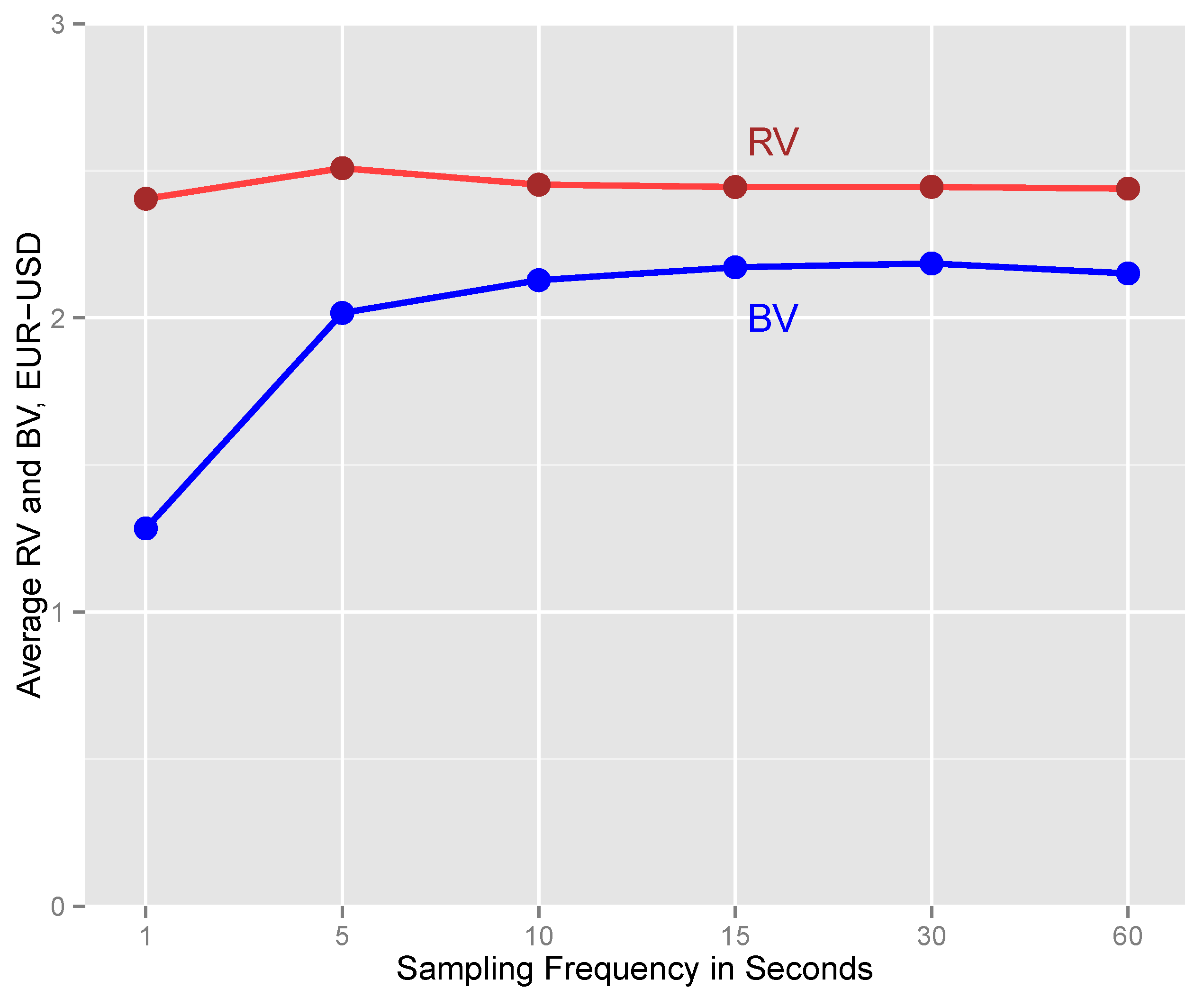
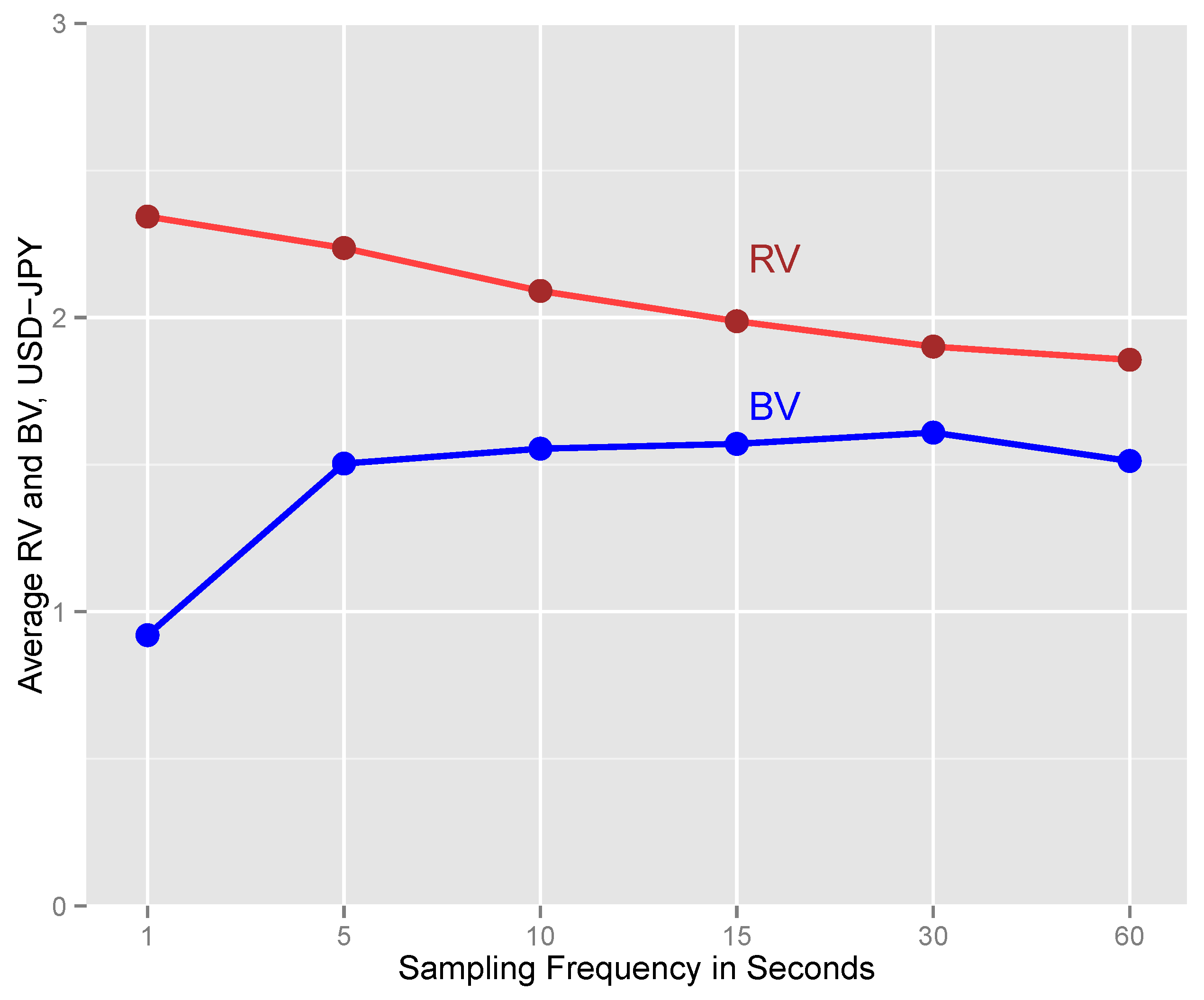
• Choose the highest sampling frequency that is free of microstructure noise by computing the quantity given by Equation (4) across different frequencies.
• At the chosen frequency, estimate the jumps $\{j_i,i=1,2,\cdots \}$ using the statistic $\mathcal{S}$ of Equation (3).
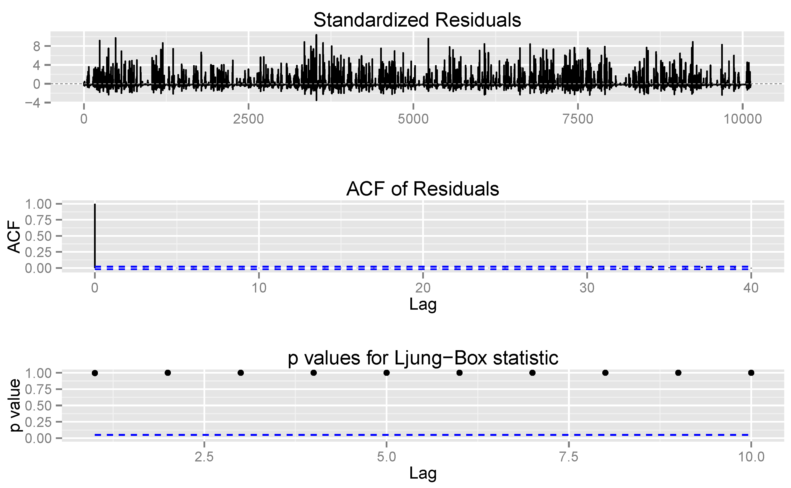
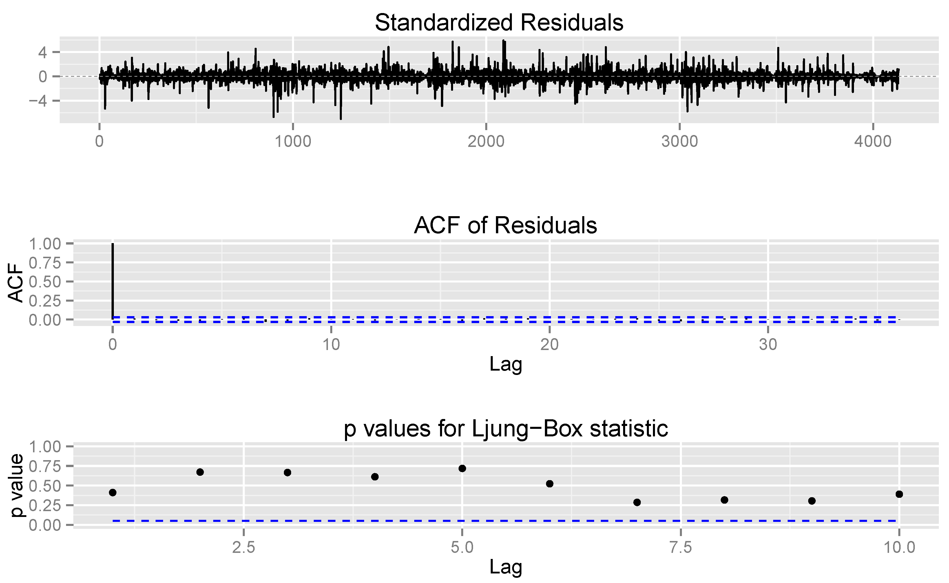
• Test the martingale null hypothesis on the time series of estimated jumps.

4. Application to FX Market

This section applies our market efficiency test in the setting of an interdealer foreign exchange market. Specifically, using our measure, we compare market efficiency before and after a tick size change. Previous studies have considered the effect of tick size change on market quality and market participant behavior in a low-frequency discrete-time framework—see, e.g., Lawrence (1991), Gwilym et al. (1998), Huang and Stoll (2001), and Ohta (2006). Our measure extends the same consideration to a high-frequency setting.

4.1. Martket Setting and Data

4.1.1. Interdealer FX Spot Market and EBS Platform

The FX market practice of trading via “vehicle currencies“ leads to concentration in trading venues and liquidity being concentrated in a handful of currency pairs. The two dominant currencies are the US dollar and Euro. The EUR/USD currency pair accounts for 28% of global FX turnover. Individually, the US dollar and Euro are involved in approximately 75% and 46% of all spot transactions, respectively. 12 The primary interdealer platform for major currency pairs—EUR/USD, USD/JPY, EUR/JPY, USD/CHF and EUR/CHF—is Electronic Broking Services (EBS), where large banks and institutions trade with each other in units of million in base currency.13 The EBS limit order books for the major currency pairs are where price discovery occurs for global spot FX trading.14

4.1.2. Data

The dataset we used consists of the EBS limit order book at a 100-millisecond frequency for major currency pairs. This is the same as tick-frequency snapshots of the limit order book observed in real-time by traders. The period we analyzed was the two-year period from January 2010 to December 2011. For each major currency pair, we had an exchange rate time series of a sample size of approximately 500 million and approximately 24–36 million recorded transactions. The transaction prices were the highest buying or lowest selling deal price between two consecutive snapshots of the order book, rounded to 100 milliseconds. The FX market operates continuously and each trading day is 24 h, beginning and ending at 17:00 US Eastern Standard Time (21:00 Greenwich Mean Time). We excluded thin weekend trading periods and holidays, as the liquidity can be limited during these periods. We present our results for the EUR/USD currency pair, for space considerations.15

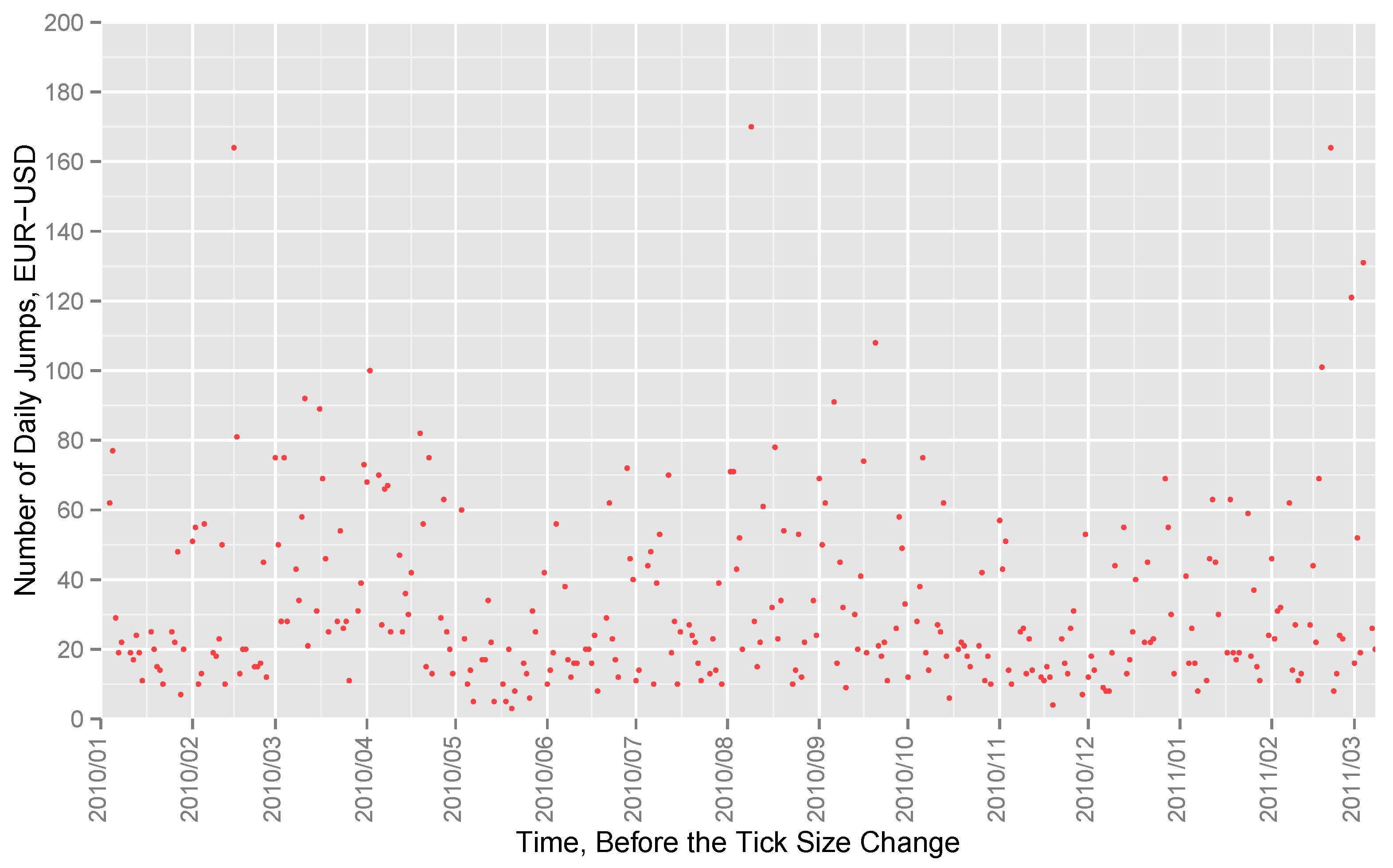
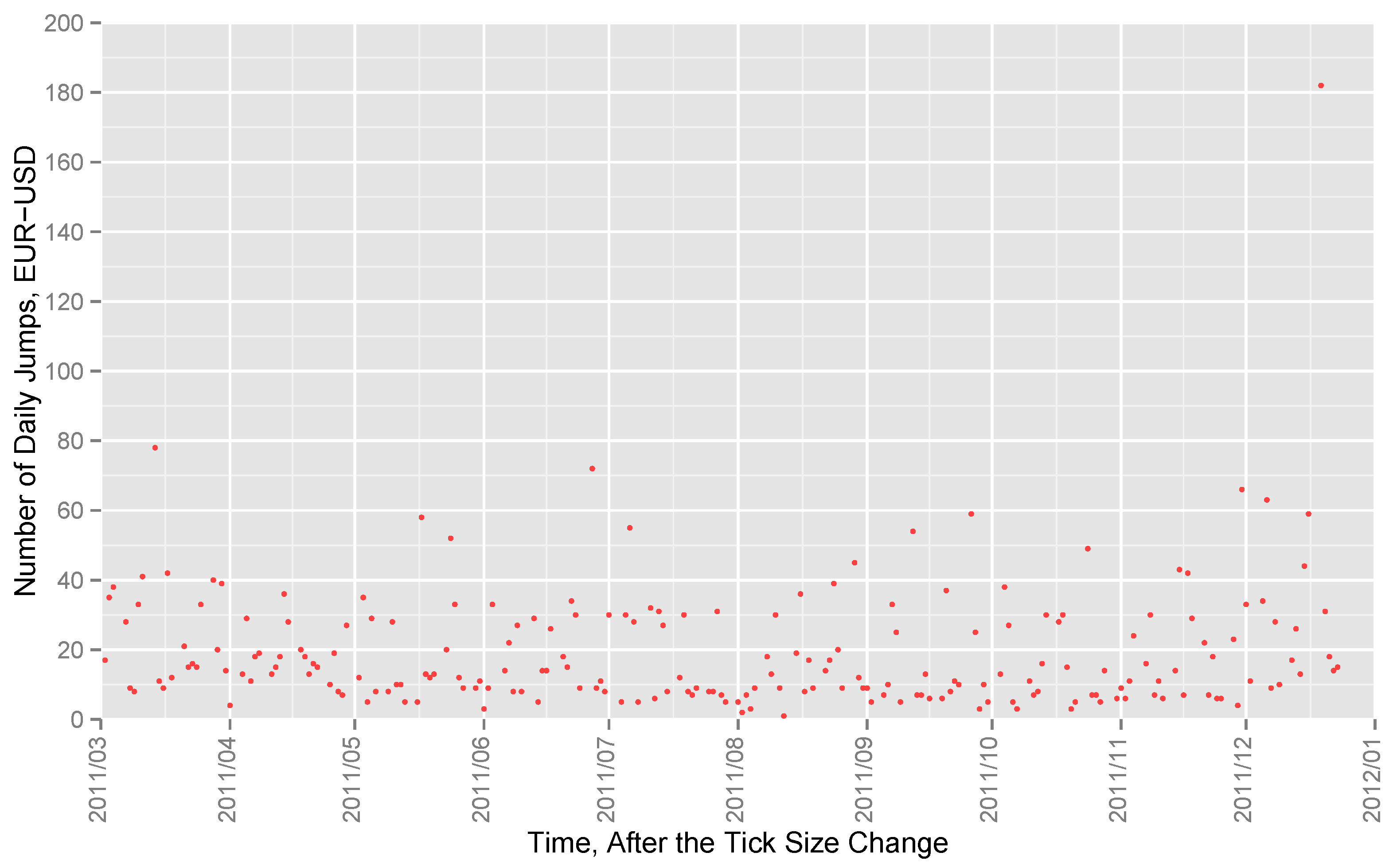
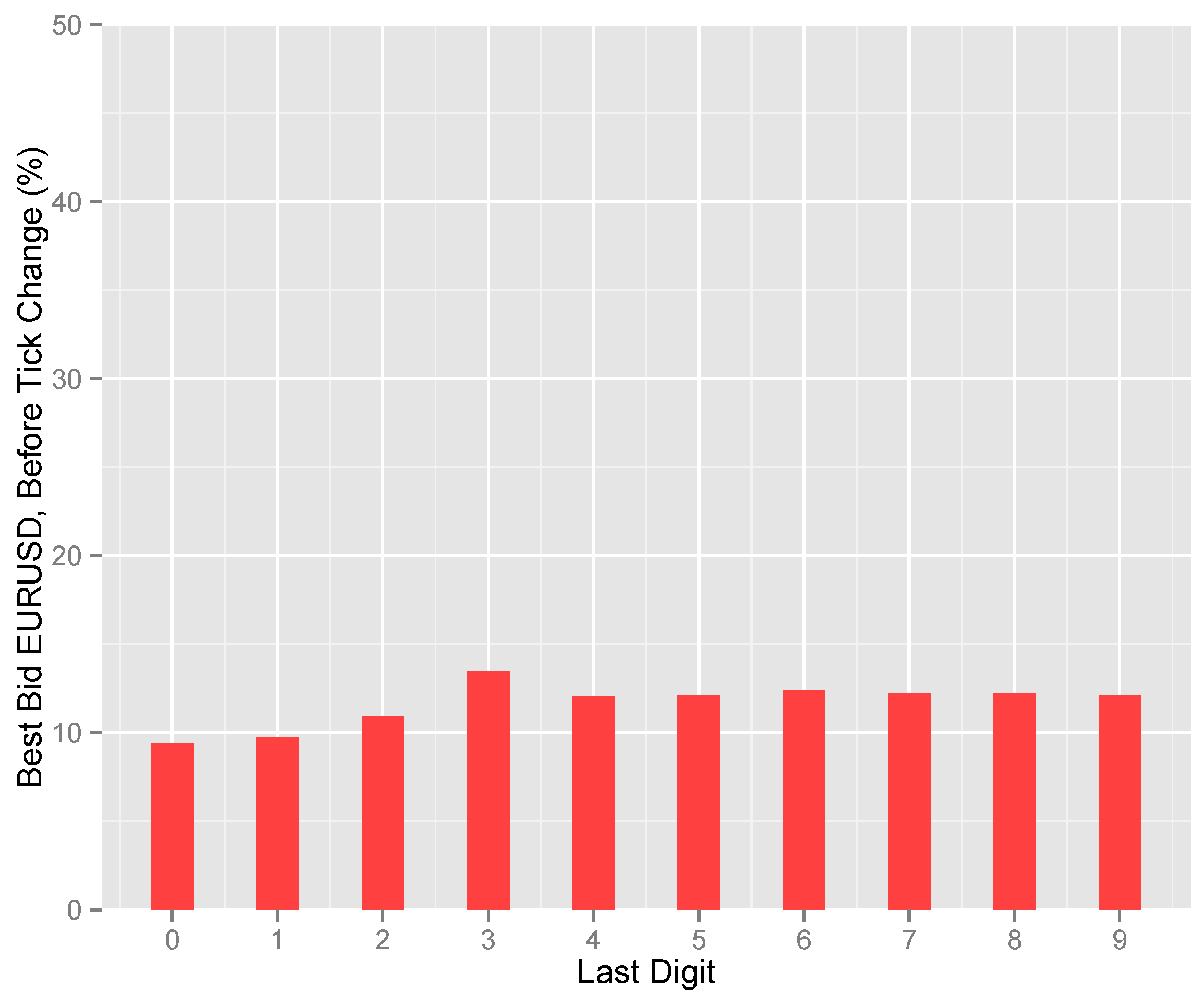
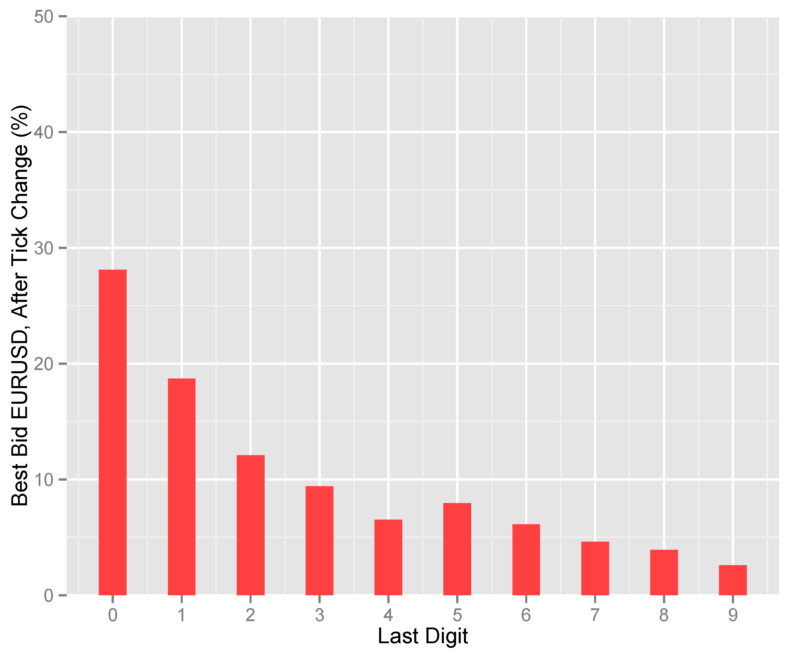
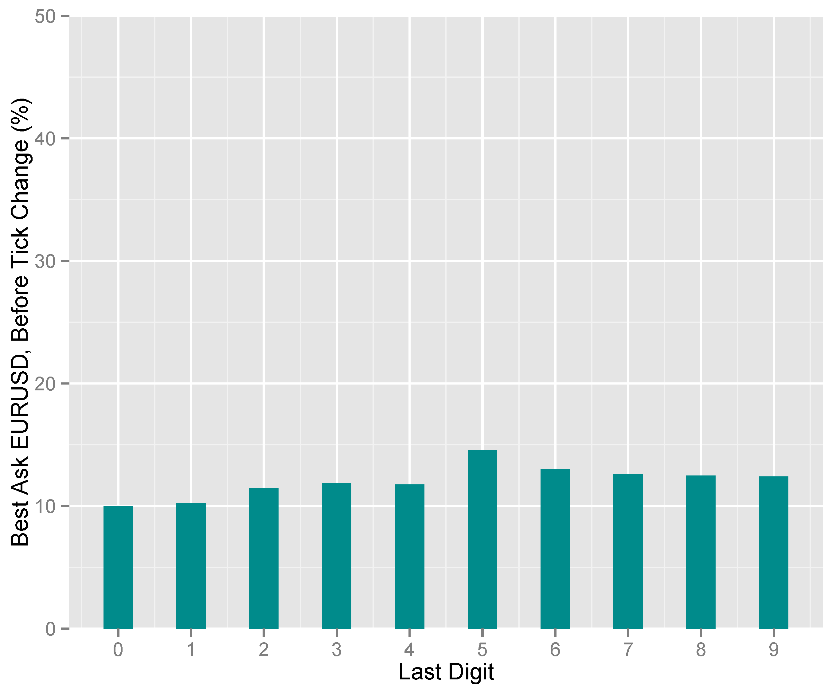
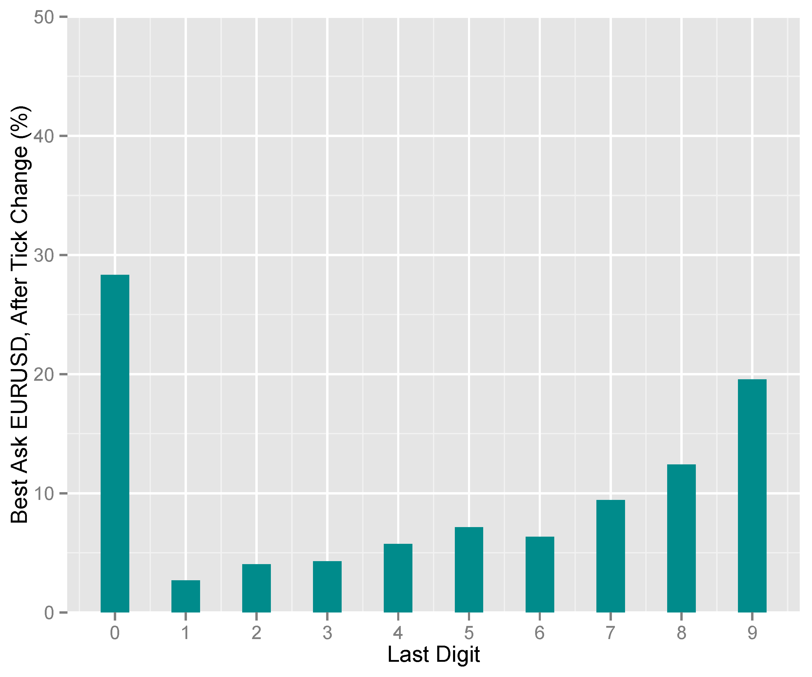
4.1.3. Tick Size Change

On 7 March 2011, EBS implemented a change in tick size, i.e., minimum price increment, from four to five decimal places—from pip to decimal pip pricing, in FX market vernacular.16 This decimalization of tick size led to a fundamental change in the high-frequency property of exchange rates. We will test the information efficiency hypothesis before and after this event.

4.2. Information Efficiency Hypothesis

4.2.1. Microstructure Noise Threshold

We chose an appropriate sampling frequency to filter out microstructure noise by comparing the difference between realized volatility and bipower variation, as defined in Equation (4), across different frequencies. For EUR/USD, the difference between hourly averages of realized volatility and bipower variation at different frequencies is shown in Figure 1.17 Figure 2 shows the same plot for USD/JPY. For all major currency pairs, the difference stabilizes at the same frequency—30 s—which was chosen as the sampling frequency. Microstructure noise became absent at the same frequency threshold for all five major currency pairs. The magnitude of the stabilized gap decreased with respect to the degree of liquidity of the currency pair. The pair with the most liquid currency, EUR/USD, had the smallest difference between realized volatility and bipower variation at the stabilized frequency of 30 s. As expected, the more liquid was found in a currency pair, the more of its variation was due to the continuous part of the exchange rate process, instead of the jump component.

4.2.2. Information Efficiency and Tick Size Change

We now apply the information efficiency hypothesis test to exchange rates before and after tick size change. From an exchange rate series sampled at a 30-second frequency, jumps were estimated and tested under the martingale null hypothesis. For the EUR/USD currency pair, the jump-testing procedure showed that there are 10150 and 4214 jumps before and after tick size change, respectively. Figure 3 and Figure 4 shows the daily time series of number of jumps, spanning the two-year sample period of 2010-2011. The martingale property of the estimated jumps was tested using the frequency-domain test of Durlauf (1991). Before a tick size change, the martingale hypothesis was rejected at the 5%-level of significance and not rejected with a large p-value of $0.64$ after tick size change. Therefore, the market became informationally efficient after tick size change. This result is reinforced by tests of serial correlation.18 Standard battery of serial correlation tests—the Box-Ljung, Box-Pierce, and Durbin-Watson tests—were also applied to the jump time series before and after tick size change. All were rejected at the 5%-level before tick size change and none were rejected after tick size change. Therefore, we conclude that market was not efficient before tick size change and became efficient after tick size change. Results are summarized in the top block of

Table 1. Jump Component of EUR/USD Process Before and After Tick Size Change.

Jump Time Series	Before	After
Durlauf Test	$p=0.0245$	$p=0.6438$
Box-Ljung Test	$p=0.0055$	$p=0.8185$
Box-Pierce Test	$p=0.0356$	$p=0.4681$
Durbin-Watson Test	$p=0.0177$	$p=0.2297$
Inter-Arrival Times	Before	After
Daily average number of jumps	33	20
Arrival intensity (exponential fit)	$3.98\times {10}^{-4}$	$2.35\times {10}^{-4}$
Autoregressive order	27	2
Jump Sizes	Before	After
Mean	$6.28\times {10}^{-6}$	$1.05\times {10}^{-5}$
Standard deviation	$3.68\times {10}^{-4}$	$4.49\times {10}^{-4}$
Skewness	$1.19$	$-0.13$
Kurtosis	$67.61$	$4.54$
Mira symmetry Test	$p=0.0000$	$p=0.3928$

.

Figure 3 and Figure 4 show the time series plot of the number of daily jumps before the tick size change, respectively.

4.3. Further Evidence

Other observed changes in exchange rate series before and after tick size change further support the conclusion of Section 4.2.

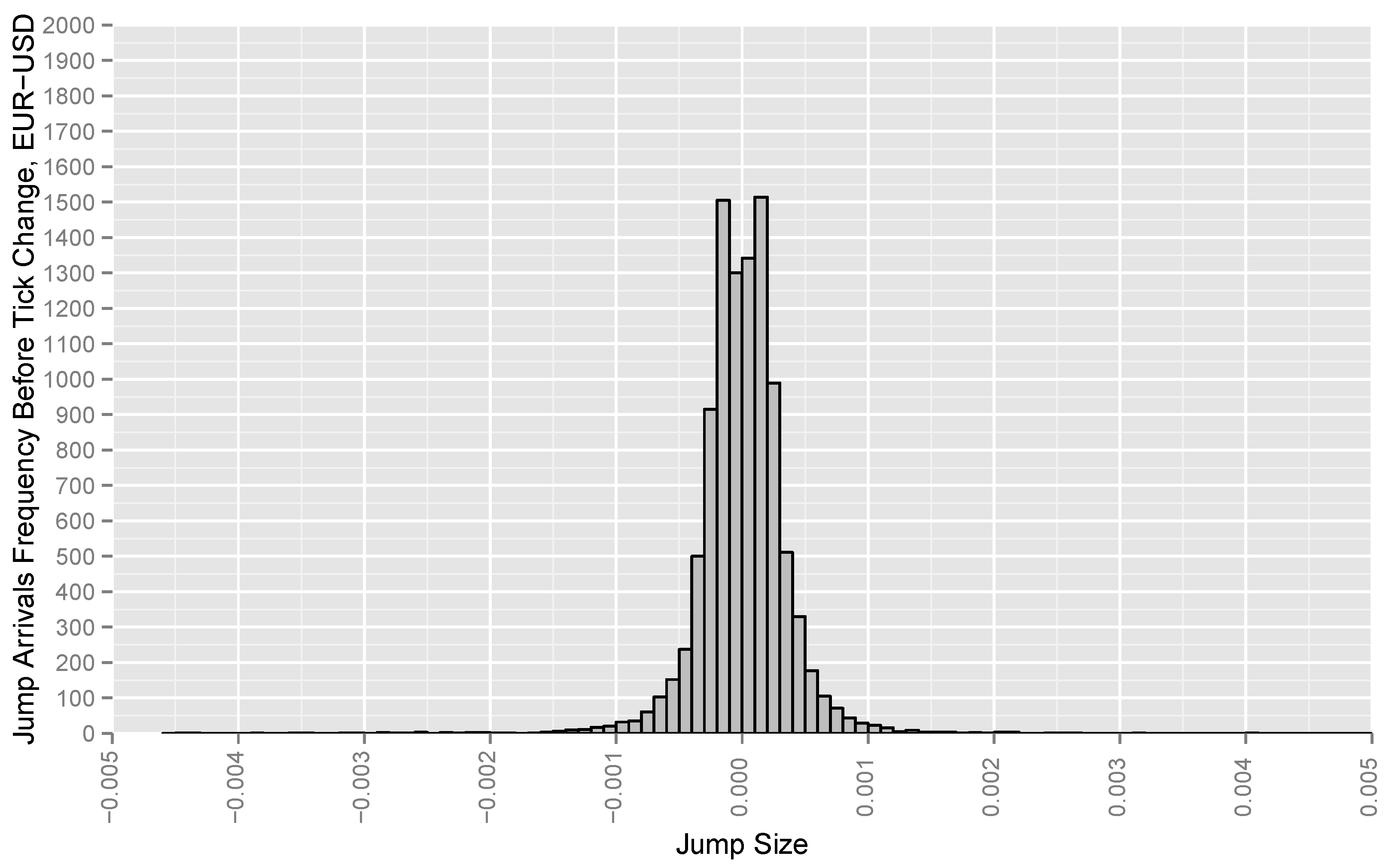
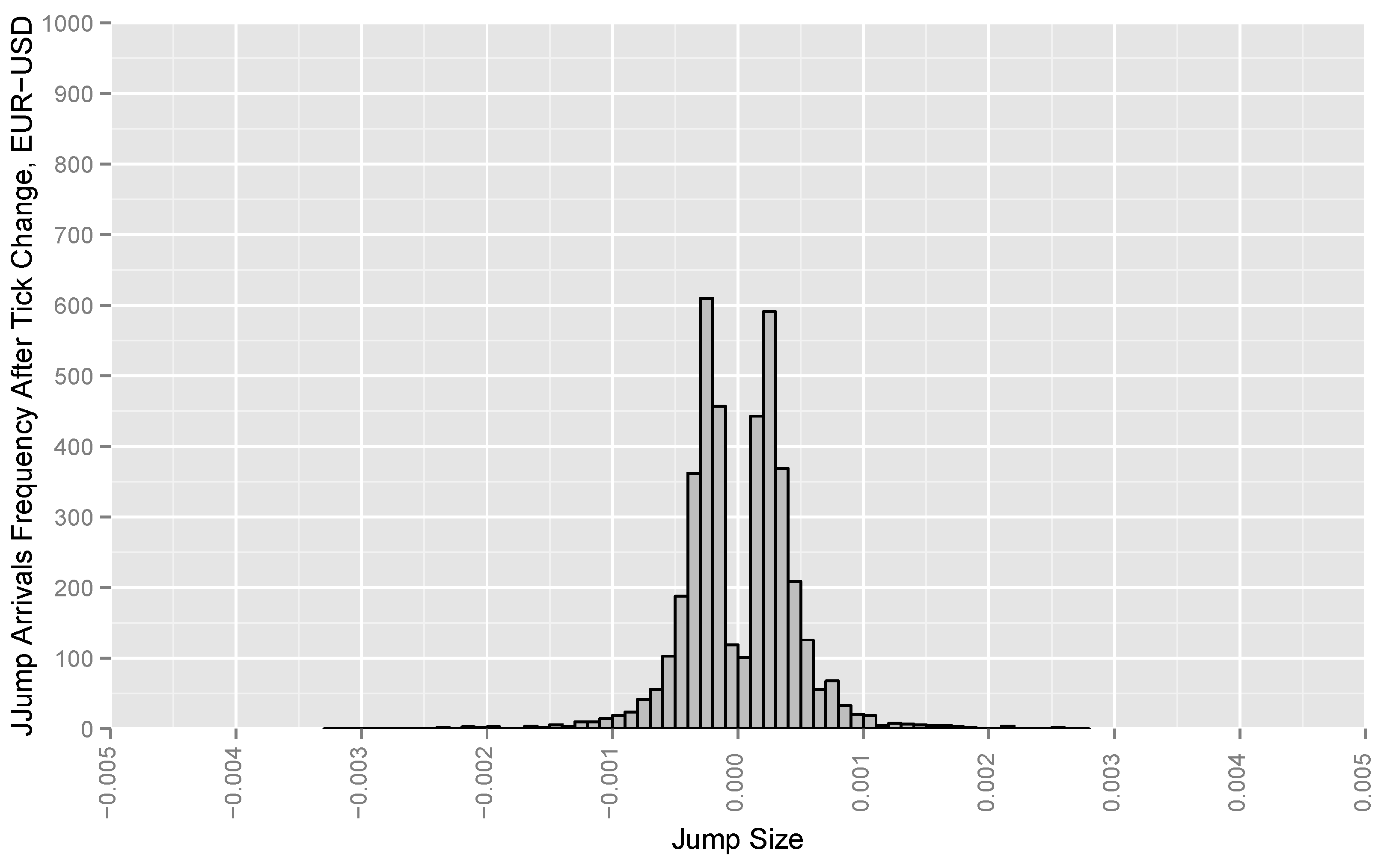
4.3.1. Jump Magnitudes

Figure 5 and Figure 6 show the histogram of jumps for EUR/USD, i.e., the cross-sectional distribution of jump sizes, before and after tick size change, respectively. Not surprisingly, the introduction of decimal pip cuts a neighborhood of around zero from the distribution of jump sizes. The size of a typical jump, measured by the standard deviation of the series, remained around 4 pip before and after decimalization. While the mean jump sizes were statistically zero, both before and after tick size change, the Mira test for symmetry rejected the symmetry hypothesis before tick size change at $p=0$ and did not reject this after tick size change. Before tick size change, jumps were heavy-tailed and skewed toward the positive side. Jumps in the exchange rate clearly became a symmetric distribution centered at zero after tick size change. Results are summarized in the bottom block of Table 1.

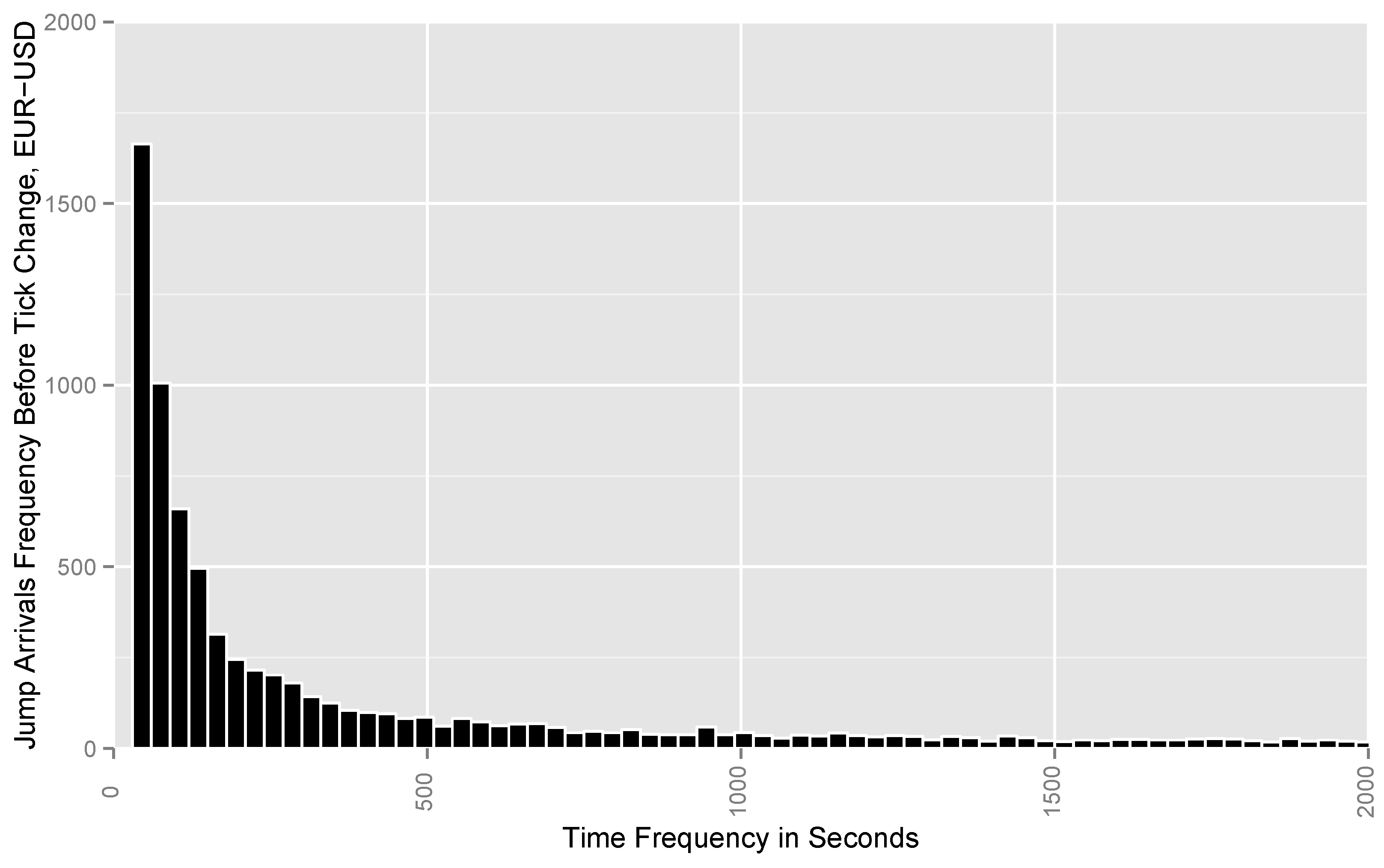
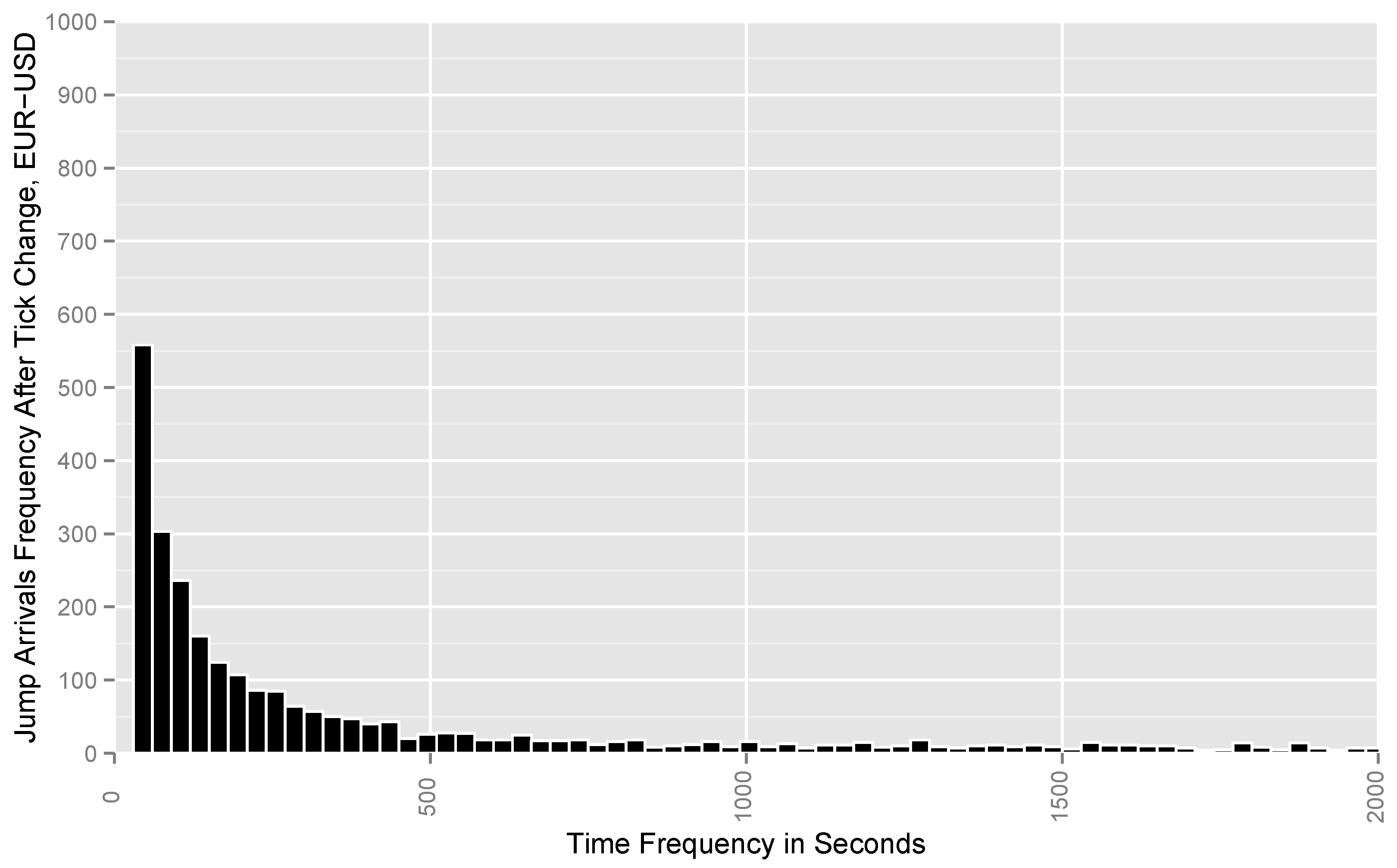
4.3.2. Jump Inter-Arrival Times

Figure 7 and Figure 8 show the histograms of inter-arrival times of jumps before and after tick size change. Both can be reasonably fitted by exponential distributions. The arrival intensity parameters from the exponential fits is lower after tick size change—see the second block of Table 1. The degree of autocorrelation of inter-arrival times also exhibits material difference before and after tick size change. Fitting auto-regressive models to the before and after inter-arrive times series yields AR(27) and AR(2) models, respectively. Therefore, the autoregressive lag decreased sharply across tick size changes. Diagnostic tests of residuals, shown in Figure 9 and Figure 10, confirm model specification of the autoregressive model. This means that the arrivals of jumps in exchange rate became significantly less clustered after tick size change.

Figure 5 and Figure 6 show the histograms of jump sizes before and after tick size change, respectively.

Figure 7 and Figure 8 show the histograms of jump inter-arrival times before and after tick size change, respectively. Exponential distributions are fitted, with results shown in the middle block of Table 1.

Autoregressive time series fit and diagnostics for jump inter-arrival times. The Akaike Information Criterion achieved the minimum value of zero for the chosen AR orders, indicating the correct specification.

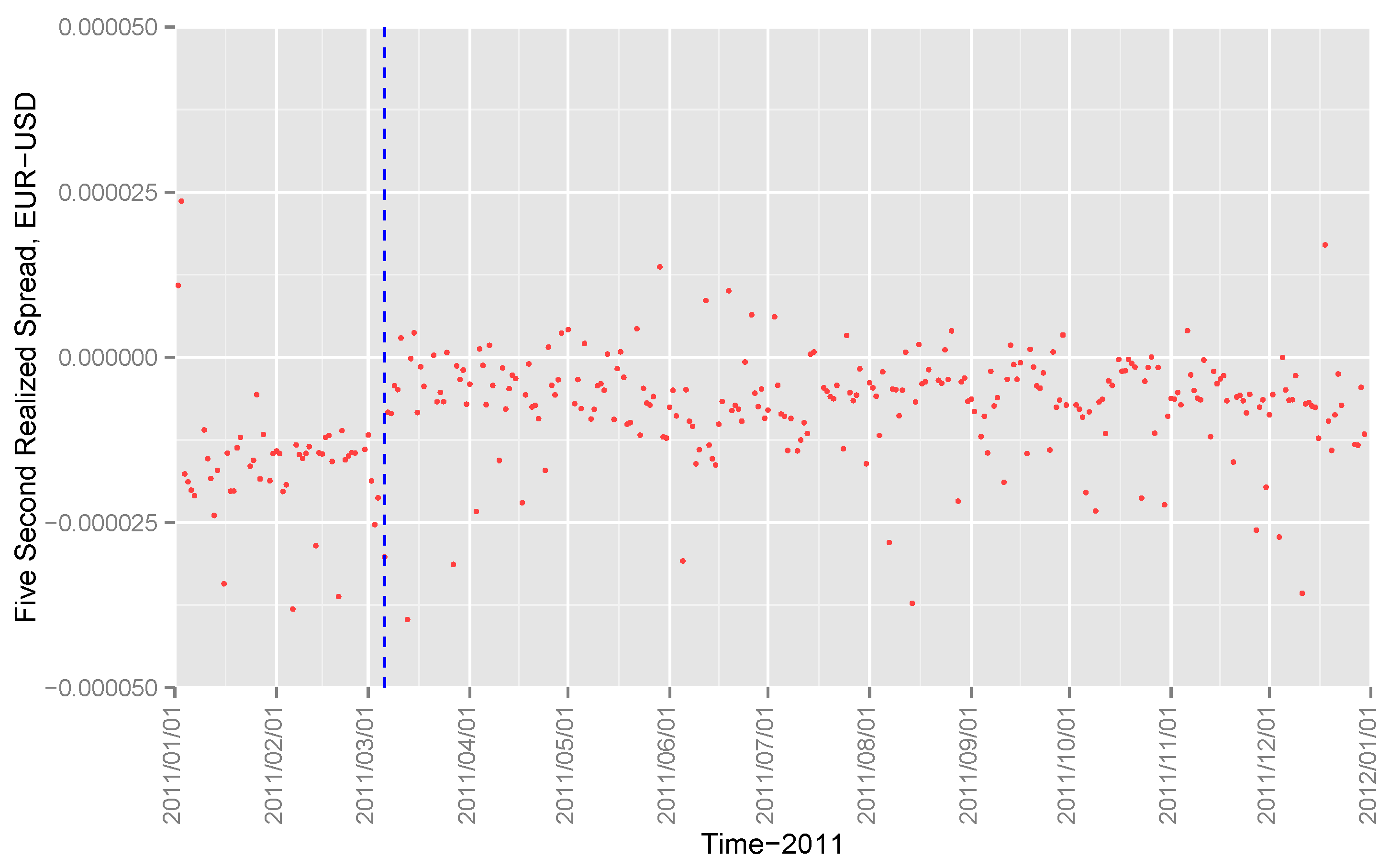
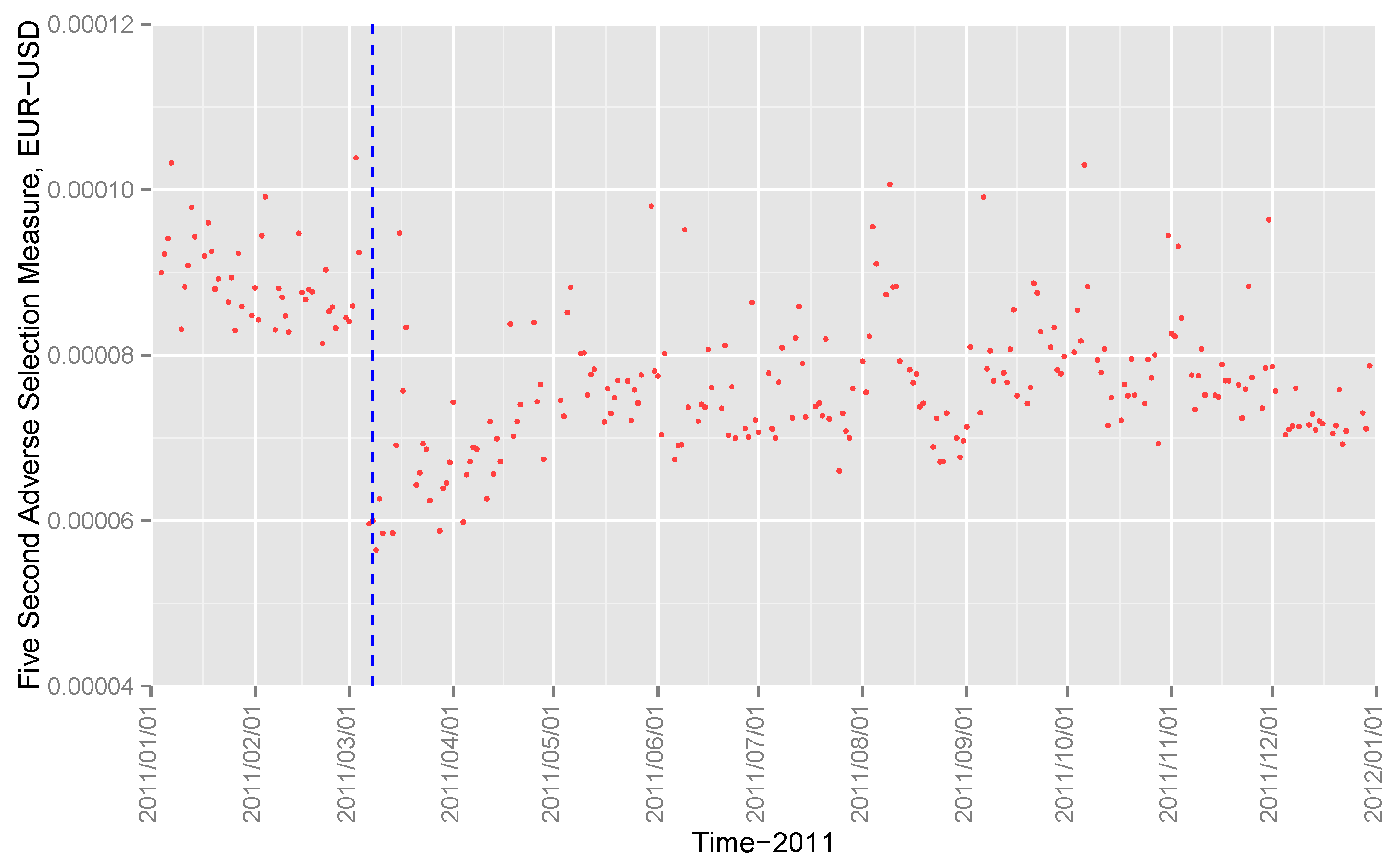
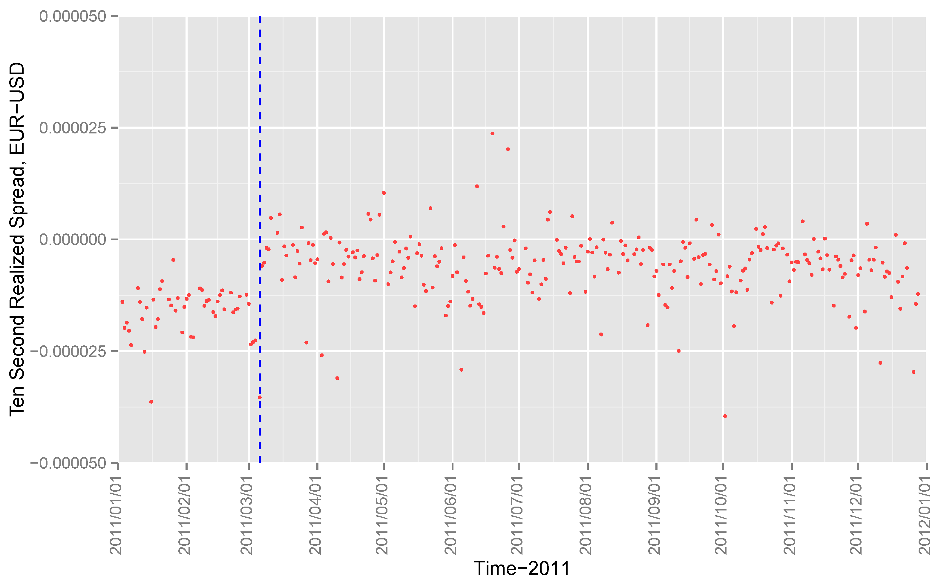
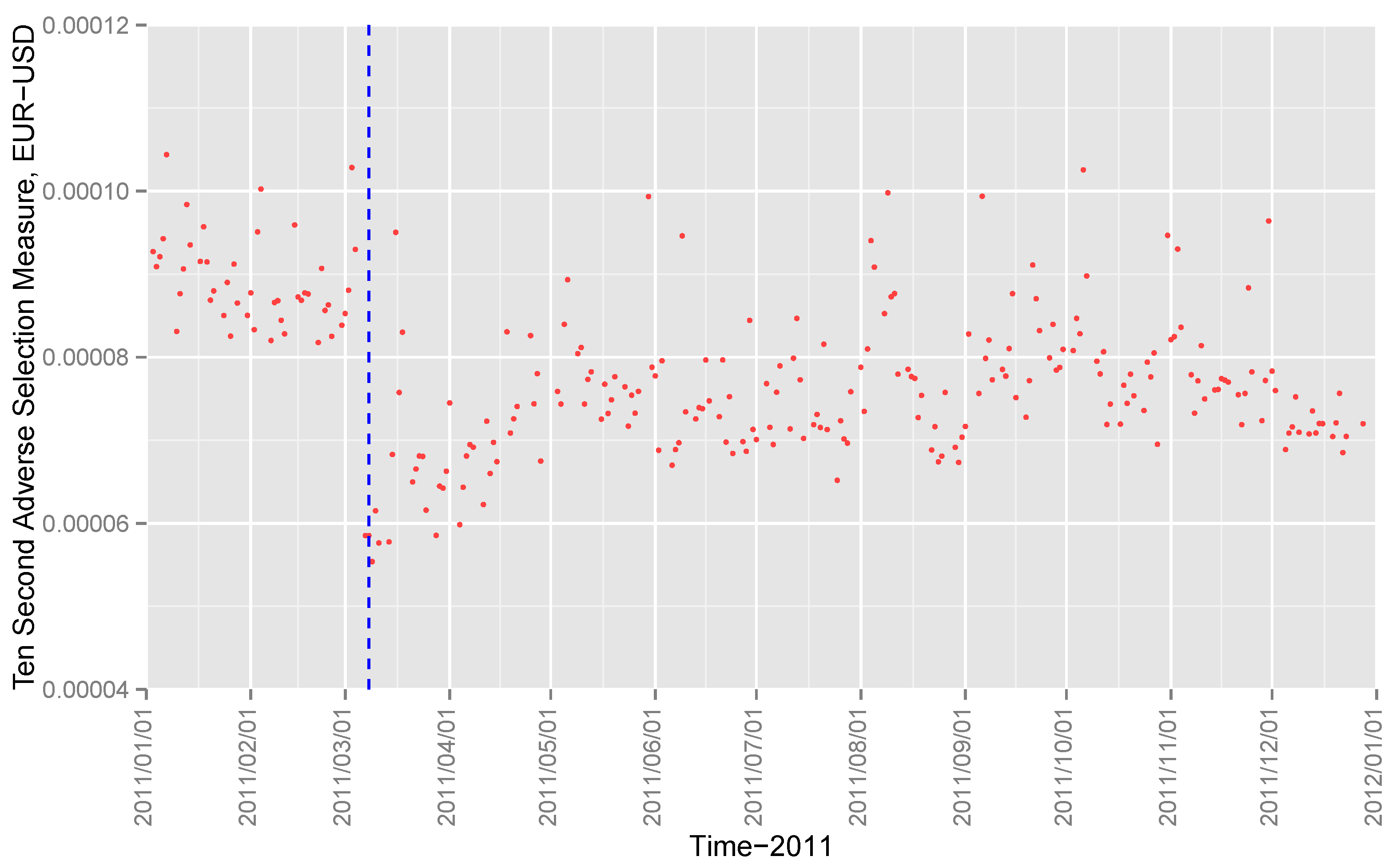
4.3.3. Realized and Effective Spreads

We also considered two standard measures of adverse selection—realized and effective spreads—before and after tick size change. This was complementary to our analysis of jumps. While jumps corresponded to a large-order flow, realized and effective spreads also reflect price movement due to a small-order flow. The spread realized at time t, denoted by $R{S}_t$, is defined by

$$R{S}_t=2Q_t(P_t-M_{t+s})$$

where $P_t$ is the transaction price at time t, $Q_t$ is the trade direction indicator, and $M_{t+s}$ is the midpoint at time $t+s$ for a chosen time interval s. $R{S}_t$ is the difference between current deal price and the quoted midpoint at a future time. After a transaction at time t, price movements favorable to the market-maker from t to $t+s$ result in a positive $R{S}_t$, and vice versa.

Realized spread was measured at a 5-second lag in Figure 11 and computed using 1.3 million deals before the tick size change and 7.3 million deals after the tick size change. Time series of daily averages are plotted. Tick size change is demarcated by a blue line. Adverse selection proxy before and after tick size change in Figure 12 shows a clear downward level shift. For all considered empirical proxies, the Chow test rejected a constant level across tick size change at $0.1\%$ level of significance.

Figure 11 shows the daily average realized spread of EUR/USD pair for 2011, before and after tick size change at 5-second frequency.19 There is a clear positive shift in realized spread across tick size change. This shows that price movement for the market marker tends to be unfavorable with a negative realized spread before tick size changes, while realized spread is nearly zero after the tick size change.

Realized spread was measured at a 10-second lag in Figure 13 and computed using 1.3 million deals before the tick size change and 7.3 million deals after the tick size change. A time series of daily averages was plotted. Tick size change is demarcated by the blue line. The adverse selection proxy before and after tick size change in Figure 14 shows a clear downward level shift.

The effective spread at time t is defined by $E{S}_t=|P_t-M_t|$, which measures the revenue of the market maker from supplying immediacy. A measure of the adverse selection of market-making is the statistic

$$E{S}_t-\frac{R{S}_t}{2}$$

i.e., revenue from supplying immediacy minus loss due to adverse price moves. Figure 12 shows a clear downward shift in the adverse selection measure for EUR/USD across tick size changes at 5-second frequency. Figure 13 and Figure 14 show identical results at 10-second frequency, for realized spread and the adverse selection measure, respectively.

Therefore, the non-rejection of the market efficiency test, together with supporting results—such as an increased symmetry in jump sizes and less clustering of jump arrivals, and the reduction in adverse selection implied by realized and effective spreads—all point to a reduction in the information content of the large-order flow. The quoted prices became more informative after a tick size change.

5. Discussion

Our measure shows that a high-frequency FX rate in the interdealer market becomes informationally efficient after a decimalization of tick size. This can be explained by the fact that the decimalization of tick size led to intensified high-frequency competition among liquidity providers, which, in turn, led to a more efficient price discovery.

There are two types of traders on the EBS platform: manual traders and automated traders. Manual traders use proprietary EBS workstations for manual order management.20 Automated traders—e.g., proprietary trading firms specializing in high-frequency trading—place orders algorithmically with little or no human intervention.21 It is known that automated (high-frequency) market makers mostly submit limit orders of the minimum size of one million, while manual market makers place larger limit orders—in fact, all orders larger than 4 million are from the manual market-makers (see Schmidt (2012)).

After tick size changes, one additional decimal place (the fifth) became available to quote prices. However, only high-frequency market makers made use of the additional decimal place. As a result, the top of the limit order book, the best bid and ask, became dominated by high-frequency traders. In the context of our dataset, this can be inferred by examining the placement of best bid and ask quotes, as well as order sizes at the best bid and ask.

The placement of best bid and ask quotes can be analyzed by examining the last digits of the best bid and ask prices. After tick size change, a last digit of zero corresponds to prices quoted at a pre-decimalized level. Figure 15 and Figure 16 show the last digits of the best bid prices before and after decimalization, respectively. Before decimalization, last digits are uniformly distributed—all market-makers make equal use of the available prices when placing quotes. After decimalization, the distribution of last digits undergo a clear change, with approximately $30\%$ concentrated at 0. Therefore, $30\%$ of the best quotes were placed at pre-decimalized levels and $70\%$ of the best quotes were placed using the newly available fifth decimal place. Figure 17 and Figure 18 show the same findings on the ask side.

By considering the order sizes at the best bid and ask, it can be further inferred that $70\%$ of the best quotes at newly decimalized levels the can be attributed to high-frequency traders.

Table 2. Size of Average Order (Million) at the Best Bid.

Last digit of quoted price	0	1	2	3	4	5	6	7	8	9
Before tick size change	1.59	1.43	1.57	1.52	1.54	1.61	1.54	1.60	1.50	1.41
After tick size change	2.12	1.06	1.05	1.08	1.08	1.58	1.05	1.01	1.07	1.10

shows the average order size at the best bid and the last digits of the best bid, before and after decimalization. Before decimalization, the average order size is uniformly distributed with respect to last digits. After decimalization, average order size at prices with the last digit zero, i.e., at pre-decimalized levels, is twice as large as those at the newly available decimal levels. In fact, orders placed at the newly available decimal level have an average size very close to the minimum order size of one million. That is, whenever a best quote is placed using the newly available fifth decimal place ($70\%$ of the time), it is very likely to have the minimal size of one million, suggesting a quote attributable to a high-frequency trader.

Table 3. Size of Average Order (Million) at the Best Ask.

Last digit of quoted price	0	1	2	3	4	5	6	7	8	9
Before tick size change	1.53	1.32	1.62	1.59	1.45	1.54	1.53	1.54	1.43	1.48
After tick size change	2.19	1.03	1.02	1.10	1.09	1.32	1.06	1.04	1.07	1.09

shows very similar results for the best ask. This suggests that manual traders price-clustered at pre-decimalized levels and effectively conceded the top of the limit order book to high-frequency traders $70\%$ of the time.

In view of the above discussion, our result is in line with other findings in the literature regarding the impact of high-frequency trading on market quality. In particular, using EBS data from 2004 to 2008, Chaboud et al. (2014) showed that high-frequency trading activity has a negative Granger-causal effect on the serial correlation of returns and conclude that high-frequency trading activity improves market efficiency. Similar conclusions have been reached for equity markets. For example, Hendershott et al. (2011) conclude that high-frequency trading enhances the informativeness of quotes and improves liquidity in NYSE limit order books. Brogaard et al. (2014) and Hasbrouck and Saar (2013) obtained similar findings for NASDAQ.

6. Conclusions

In this paper, we incorporated considerations of price impact and information efficiency in a semimartingale framework. Our framework is a an extension of discrete-time settings, where market efficiency corresponds to the martingale property. In the high-frequency setting, the price semimartingale is the sum of a finite-variation process, a continuous local martingale, and a jump process. In other words, the price has a locally riskless component, an informationally efficient component, and a jump component. When the jump component is white noise, large orders have no permanent price impact and price is a martingale. In this high-frequency framework, we analyze the impact of tick size decimalization on the information efficiency of the price process. Our overall analysis shows that a smaller tick size improves information efficiency.

As the speed and latency envelope of today’s markets continue to evolve, and high-frequency data continue to become more widely available, questions regarding market quality remain of fundamental interest and require continuous adaption of the empirical toolset used to address the issue.22 Our measure of information efficiency contributes to this endeavor. Extending such considerations to the full limit order book, and further to multiple limit order books, remains to be explored in future research.23

[custom]

References

1. Aït-Sahalia, Yacine, and Jean Jacod. 2009. Estimating the degree of activity of jumps in high frequency data. Annals of Statistics 37: 2202–44. [Google Scholar] [CrossRef] [Green Version]
2. Amihud, Yakov. 2002. Illiquidity and stock returns: Cross-section and time-series effects. Journal of Financial Markets 5: 31–56. [Google Scholar] [CrossRef] [Green Version]
3. Andersen, Torben G., Tim Bollerslev, and Dobrislav Dobrev. 2007a. No-arbitrage semi-martingale restrictions for continuous-time volatility models subject to leverage effects, jumps and i.i.d. noise: Theory and testable distributional implications. Journal of Econometrics 138: 125–80. [Google Scholar] [CrossRef] [Green Version]
4. Andersen, Torben G., Tim Bollerslev, and Francis X. Diebold. 2007b. Roughing it up: Including jump components in the measurement, modeling, and forecasting of return volatility. Review of Economics and Statistics 89: 701–20. [Google Scholar] [CrossRef]
5. Andersen, Torben G., Tim Bollerslev, Per Frederiksen, and Morten Ørregaard Nielsen. 2010. Continuous-time models, realized volatilities, and testable distributional implications for daily stock returns. Journal of Applied Econometrics 25: 233–61. [Google Scholar] [CrossRef] [Green Version]
6. Barndorff-Nielsen, Ole E., and Neil Shephard. 2004. Power and bipower variation with stochastic volatility and jumps. Journal of Financial Econometrics 2: 1–37. [Google Scholar] [CrossRef] [Green Version]
7. Barndorff-Nielsen, Ole E., and Neil Shephard. 2006. Econometrics of testing for jumps in financial economics using bipower variation. Journal of Financial Econometrics 4: 1–30. [Google Scholar] [CrossRef]
8. Boudt, Kris, Christophe Croux, and Sébastien Laurent. 2011. Robust estimation of intraweek periodicity in volatility and jump detection. Journal of Empirical Finance 18: 353–67. [Google Scholar] [CrossRef]
9. Brogaard, Jonathan, Terrence Hendershott, and Ryan Riordan. 2014. High-frequency trading and price discovery. Review of Financial Studies 27: 2267–306. [Google Scholar] [CrossRef] [Green Version]
10. Cai, Jie, Ralph A. Walkling, and Ke Yang. 2016. The price of street friends: Social networks, informed trading, and shareholder costs. Journal of Financial and Quantitative Analysis 51: 801–37. [Google Scholar] [CrossRef] [Green Version]
11. Chaboud, Alain, Benjamin Chiquoine, Erik Hjalmarsson, and Clara Vega. 2014. Rise of the machines: Algorithmic trading in the foreign exchange market. Journal of Finance 69: 2045–84. [Google Scholar] [CrossRef] [Green Version]
12. Delbaen, Freddy, and Walter Schachermayer. 1994. A general version of the fundamental theorem of asset pricing. Mathematische Annalen 300: 463–520. [Google Scholar] [CrossRef]
13. Durlauf, Steven N. 1991. Spectral based testing of the martingale hypothesis. Journal of Econometrics 50: 355–76. [Google Scholar] [CrossRef] [Green Version]
14. Fama, Eugene F. 1970. Efficient market hypothesis: A review of theory and empirical work. Journal of Finance 25: 28–30. [Google Scholar] [CrossRef]
15. Fama, Eugene F. 1991. Efficient markets: Ii. fiftieth anniversary invited paper. Journal of Finance 46: 1575–617. [Google Scholar] [CrossRef]
16. Gu, Chen, and Alexander Kurov. 2020. Informational role of social media: Evidence from twitter sentiment. Journal of Banking and Finance. [Google Scholar] [CrossRef]
17. Gwilym, Owain, Andrew Clare, and Stephen Thomas. 1998. Extreme price clustering in the London equity index futures and options markets. Journal of Banking & Finance 22: 1193–206. [Google Scholar]
18. Harrison, J. Michael, and David M Kreps. 1979. Martingales and arbitrage in multiperiod securities markets. Journal of Economic Theory 20: 381–408. [Google Scholar] [CrossRef]
19. Hasbrouck, Joel, and Gideon Saar. 2013. Low-latency trading. Journal of Financial Markets 16: 646–79. [Google Scholar] [CrossRef]
20. Hendershott, Terrence, Charles M. Jones, and Albert J. Menkveld. 2011. Does algorithmic trading improve liquidity? Journal of Finance 66: 1–33. [Google Scholar] [CrossRef] [Green Version]
21. Huang, Roger D., and Hans R. Stoll. 1997. The components of the bid-ask spread: A general approach. Review of Financial Studies 10: 995–1034. [Google Scholar] [CrossRef]
22. Huang, Roger D., and Hans R. Stoll. 2001. Tick size, bid-ask spreads, and market structure. The Journal of Financial and Quantitative Analysis 36: 503–22. [Google Scholar] [CrossRef] [Green Version]
23. Jing, Wei, and Xueyong Zhang. 2021. Online social networks and corporate investment similarity. Journal of Corporate Finance 68: 101921. [Google Scholar] [CrossRef]
24. Kyle, Albert S. 1985. Continuous auctions and insider trading. Econometrica 53: 1315–35. [Google Scholar] [CrossRef] [Green Version]
25. Lawrence, Harris. 1991. Stock price clustering and discreteness. Review of Financial Studies 4: 389–415. [Google Scholar]
26. Lee, Suzanne S., and Jan Hannig. 2010. Detecting jumps from lévy jump diffusion processes. Journal of Financial Economics 96: 271–90. [Google Scholar] [CrossRef] [Green Version]
27. Lee, Suzanne S., and Per A. Mykland. 2008. Jumps in financial markets: A new nonparametric test and jump dynamics. Review of Financial Studies 21: 2535–63. [Google Scholar] [CrossRef]
28. Marazzi, Alfio, and Victor J Yohai. 2004. Adaptively truncated maximum likelihood regression with asymmetric errors. Journal of Statistical Planning and Inference 122: 271–91. [Google Scholar] [CrossRef]
29. O’Hara, Maureen. 2015. High frequency market microstructure. Journal of Financial Economics 116: 257–70. [Google Scholar] [CrossRef]
30. Ohta, Wataru. 2006. An analysis of intraday patterns in price clustering on the Tokyo Stock Exchange. Journal of Banking & Finance 30: 1023–39. [Google Scholar]
31. Schmidt, Anatoly B. 2012. Ecology of the Modern Institutional Spot FX: The EBS Market in 2011. SSRN. Available online: http://ssrn.com/abstract=1984070 (accessed on 15 December 2021).
32. White, Halbert. 2014. Asymptotic Theory for Econometricians. Cambridge: Academic Press. [Google Scholar]
Figure 1. RV-BP, EUR/USD.
Jrfm 15 00097 g001
Figure 2. RV-BP, USD/JPY.
Jrfm 15 00097 g002
Figure 3. Daily Number of Jumps of EUR/USD, Before Tick Size Change.
Jrfm 15 00097 g003
Figure 4. Daily Number of Jumps of EUR/USD, After Tick Size Change.
Jrfm 15 00097 g004
Figure 5. Jump Sizes of EUR/USD, Before Tick Size Change.
Jrfm 15 00097 g005
Figure 6. Jump Sizes of EUR/USD, After Tick Size Change.
Jrfm 15 00097 g006
Figure 7. Jump Inter-Arrival Times Before Tick Size Change, EUR/USD.
Jrfm 15 00097 g007
Figure 8. Jump Inter-Arrival Times After Tick Size Change, EUR/USD.
Jrfm 15 00097 g008
Figure 9. Jump Inter-Arrival Times, Before Tick Size Change.
Jrfm 15 00097 g009
Figure 10. Jump Inter-Arrival Times, After Tick Size Change.
Jrfm 15 00097 g010
Figure 11. EUR/USD Realized Spread, Five-Second Frequency.
Jrfm 15 00097 g011
Figure 12. EUR/USD Adverse Selection Proxy, Five-Second Frequency.
Jrfm 15 00097 g012
Figure 13. EUR/USD Realized Spread, Ten-Second Frequency.
Jrfm 15 00097 g013
Figure 14. EUR/USD Adverse Selection Proxy, Ten-Second Frequency.
Jrfm 15 00097 g014
Figure 15. Best Bid Last Digits, Before Tick Change.
Jrfm 15 00097 g015
Figure 16. Best Bid Last Digits, After Tick Change.
Jrfm 15 00097 g016
Figure 17. Best Ask Last Digits, Before Tick Change.
Jrfm 15 00097 g017
Figure 18. Best Ask Last Digits, After Tick Change.
Jrfm 15 00097 g018