Spatial Analysis and Modeling of the Housing Value Changes in the U.S. during the COVID-19 Pandemic

Abstract

COVID-19 has affected almost all sectors of the economy, including the real estate markets across different countries in the world. A rich body of literature has emerged in analyzing real estate market trends and revealing important information. However, few studies have used a spatial perspective to investigate the impact of COVID-19 on property values. The main purposes of this study are as follows: (1) to explore the spatial distribution and spatial patterns of housing price changes during the COVID-19 pandemic crisis in the U.S. real estate market and (2) to model the spatially nonstationary relationships between the housing price change and COVID-19 characteristics. We find that housing price changes differ across space and appear associated with the spatial distribution of the COVID-19 case rates. The housing market volatility is amplified by the uneven distribution of some socioeconomic factors. The spatially uneven housing price changes may bring an uneven spillover effect to the rest of the economy and lead to divergence in economic growth across different areas.

1. Introduction

Since the initial outbreak of COVID-19, the pandemic has generated severe global economic disruptions. These disruptions have resulted in one of the largest economic recessions in the United States (U.S.) since the Great Depression (Del Giudice et al. 2020). COVID-19 has affected almost all sectors of the economy, including the real estate markets across different countries in the world (Nicola et al. 2020). Governments across the world developed different policies to fight the negative consequences of the pandemic crisis on the housing market (Kholodilin 2020). Since home equity is the single largest financial asset for most households and numerous jobs are connected with the real estate sector, structural breaks in property values may lead to even more profound macroeconomic and microeconomic consequences. Housing price changes can play an important role in fueling the growth or decline of the economy. For example, the cooling of the housing market triggered an economic recession in 2007. Previous studies found strong effects of housing prices on economic consumption and production (Case et al. 2005; Miller et al. 2011a, 2011b). Notably, the recent changes in the real estate market during the COVID-19 pandemic have produced speculation of an urban exodus in the current socioeconomic climate. As the emphasis on properly conducting safety measures necessary to mitigate the impacts of COVID-19 grows, many people have become circumspect in terms of their daily choices. Concerning pandemic restrictions have led city-dwellers to reevaluate where to reside. As densely populated neighborhoods are at higher risk of spreading COVID-19, the desire to relocate to a city’s less dense suburbs has dramatically increased (Liu and Su 2021; Ramani and Bloom 2021; Li and Zhang 2021). A key economic evaluation arises as to whether the desire for living in rural or suburban neighborhoods, where individuals have greater freedom and safety from disease, outweighs the economic opportunities in urban areas that held significant merits over the former prior to the pandemic.

The study of pandemic-induced fundamental changes in consumer behavior along with other key real estate issues has generated substantial scholarly interest (Goodman and Magder 2020). A rich body of literature has emerged in analyzing market trends and revealing important information (Kuk et al. 2021; Verhaeghe and Ghekiere 2021). Balemi et al. (2021) provided a comprehensive literature review of the latest academic insights into how this pandemic has affected housing, commercial real estate, and the mortgage market. Hoesli and Malle (2021) analyzed the effects of the COVID-19 pandemic on commercial real estate prices, particularly in European markets, emphasizing the differences across property types. In the Middle East, Ahsan and Sadak (2021) and Tanrıvermiş (2020) examined the possible effects and impacts of the COVID-19 outbreak on Turkish real estate development. In Oceania, Hu et al. (2021) inspected COVID-19’s effect on Australian housing prices considering two factors: epidemiological severity and policy intervention. In Europe, Verhaeghe and Ghekiere (2021) studied the impact of the COVID-19 pandemic on ethnic discrimination in the housing market of a metropolitan city in Belgium. Marona and Tomal (2020) assessed the impact of the COVID-19 pandemic upon the workflow of real estate brokers and their clients’ attitudes in Krakow, Poland. Del Giudice et al. (2020) and De Toro et al. (2021) evaluated the short- and mid-run COVID-19 effects on housing prices in Italy. Blakeley (2021) and Uchehara et al. (2020) provided a wide-ranging insight into the effects of the COVID-19 crisis on real estate in the U.K. In Asia, Hamzah et al. (2020) argued that a U-shaped recovery is more likely to hit the real estate industry. Chong and Liu (2020), Qian et al. (2021), and Cheung et al. (2021) investigated the impact of COVID-19 on housing prices in China. In the U.S., Yoruk (2020) explored the early effect of the COVID-19 pandemic on the U.S. housing market. Jones and Grigsby-Toussaint (2020) acknowledged that racial and ethnic minorities experienced the worst housing outcomes of this COVID-19 pandemic. Beard (2020) recommended policy actions to mitigate the most negative impacts on housing access applicable both in Michigan and nationwide. Ling et al. (2020) and Ramani and Bloom (2021) studied the effect of COVID-19 on U.S. commercial real estate prices. D’Lima et al. (2020) provided evidence of housing market effects following government shutdown responses to COVID-19 using micro-level data on U.S. residential property transactions. Bayoumi and Zhao (2020), Wang (2021), Nicola et al. (2020), and Zhao (2020) found that the U.S. real estate market has hitherto shown little sign of distress.

Despite these studies, very few studies have used a spatial perspective to investigate the impact of COVID-19 on property values (Li and Zhang 2021; Liu and Su 2021; Ramani and Bloom 2021; Wang 2021; Yilmazkuday 2020). On the one hand, previous studies in literature showed that housing prices are spatially autocorrelated. Realtors know that “location, location, location” determines housing prices. The geographic location of a house affects access to employment, shopping, recreation, neighborhood characteristics, environmental amenities, and public services. Geographic location, therefore, affects real estate business concerning housing supply, marketing, and financing. Geographic location plays an important role in determining the market value of a property. On the other hand, infectious diseases such as COVID-19 have substantial geographic variations in range and intensity of transmission induced by the uneven geographic distribution of vulnerable populations and risk factors that facilitate the spatial dispersion of the virus. Spatial attributes, such as population density and airport and road connectivity, should be linked to the geographic disparities of COVID-19 risk and transmission rates. Urban areas with connectivity enhanced by air transport and dense populations may have a faster spread of COVID-19 infection compared to rural and less connected areas with sparse populations. Because both housing values and COVID-19 vary a great deal with different geographic locations, there might be different impacts of COVID-19 on housing values across different geographic locations.

In addition to spatial autocorrelation, housing price may also exhibit spatial heterogeneity within a large housing market due to localized supply and demand imbalances (Goodman 1981; Goodman and Thibodeau 1998). The awareness of limitations of traditional hedonic price analysis has led to the development of a wide range of spatial models accounting for spatial effects in residential data sets (Anselin et al. 1996). Spatial models explicitly account for two major spatial effects in housing prices typically ignored in global hedonic housing price models: spatial dependency and spatial heterogeneity (Anselin 1988). Geographically weighted regression (GWR) is one of these spatial models addressing spatial dependency and spatial heterogeneity (Brunsdon et al. 1996). In fact, GWR is a local spatial modeling approach that explicitly allows parameter estimates to vary over space (Brunsdon et al. 1996; Fotheringham et al. 2003). Lately, GWR has been utilized in housing price prediction (e.g., Li et al. 2016; Lu et al. 2014; Yu et al. 2007). For example, Yu et al. (2007) employed GWR to examine spatial dependence and heterogeneity of housing-market dynamics in the City of Milwaukee. Bitter et al. (2007) compared two approaches to examine spatial heterogeneity in housing attribute prices within the Tucson, Arizona, housing market: the spatial expansion method and GWR. They found that GWR outperforms the spatial expansion method in terms of explanatory power and predictive accuracy. Recently, Li and Wei (2020) used GWR to examine the local geographies of the housing value bust (2008–2012) and boom (2012–2016) since the financial crisis in Salt Lake County, Utah.

In fact, there are many publications in the literature studying the effects of past crises on the housing market, such as health epidemics (e.g., Wong 2008; Tyndall 2019; Francke and Korevaar 2021; Custodio et al. 2021; D’Lima and Thibodeau 2022) and the global financial crisis (e.g., Maclennan and O’Sullivan 2011; Murphy 2011; Forrest and Yip 2011; Jones and Richardson 2014; Grimes and Hyland 2015). Some publications studied the effects of past crises on the housing market from the spatial perspective (e.g., Aalbers 2009; Martin 2011; Li and Wei 2020). However, to the best of our knowledge, it seems that no publication has investigated the spatial relationships between COVID-19 infection and housing values, and consequently no publication has applied GWR to study the spatial relationships. This paper intends to use the GWR model for investigating the spatial impacts of COVID-19 on the housing price changes in the U.S. real estate market. We will explore the spatial dependency and spatial heterogeneity of property value changes in the U.S. during the COVID-19 pandemic. Specifically, the main purposes of this study are as follows: (1) to explore the spatial distribution and spatial patterns of housing price changes during the COVID-19 pandemic crisis in the U.S. real estate market and (2) to model the spatially nonstationary relationships between the housing price change and COVID-19 characteristics. We aim to address the following research questions: Is there a relationship between COVID-19 cases and housing price changes? If so, how significant is the relationship? How does this spatial relationship vary as regards the uneven distribution of COVID-19 characteristics and other socioeconomic variables, such as population, employment, education, and poverty data across different counties in the U.S.?

2. Data and Methodology

2.1. Data

This study used data from four primary sources: Zillow Home Index Value (ZHVI), USA Facts, the U.S. Census Bureau, and the U.S. Department of Agriculture.

Table 1. Data names and sources.

Data Types	Data Names	GIS Abbrev. Attribute Names	Data Sources
Home Value	Zillow Home Value Index (ZHVI) data 2020–2021		Zillow Research Data: https://www.zillow.com/research/data/ (accessed on 6 June 2021).
	Change rates of ZHVI from May 2020 to May 2021	C5_20_21	Calculated by authors
COVID-19 Data	Number of COVID-19 cases by 30 June 2021	COVID	USA Facts: https://usafacts.org/visualizations/coronavirus-covid-19-spread-map (accessed on 30 July 2021).
	COVID-19 rates by 30 June 2021	COVID_R
Population, Employment, Education, Poverty, and Other Socioeconomic Data	Total population	POP	U.S. Census Bureau: https://covid19.census.gov/search?collection=Dataset (accessed on 10 July 2021).
	Population density	POP_DENSITY
	Percent of households with income in the past 12 months that was less than USD 75,000	HOUSELT75KP
	Total population that worked at home	POP_WORK_HOME
	Percent of civilian employed population 16 years and over in healthcare practitioners and technical occupations	HCTOCC_CALC
	Average household size	HOUSEHOLD_SIZE
	Total civilian noninstitutionalized population with health insurance coverage	POP_INSUR
	Percent of population with no health insurance coverage	POP_NO_INSUR
	Percent of households with Internet at home	PER_ INTERNET
	Total households with a computer	HH_COMPUTER
	Total households with a broadband Internet subscription	HH_INTERNET
	Number employed annual average, 2020	EMPLOYED	U.S. Department of Agriculture: https://www.ers.usda.gov/data-products/county-level-data-sets/download-data/ (accessed on 10 July 2021).
	Bachelor degree or higher, 2015–2019	BACHELOR
	Percent of adults with a bachelor degree or higher, 2015–2019	PER_BACHELOR
	Estimate of people of all ages in poverty 2019	POVALL
	Estimate of median household income 2019	MEDHHINC
	Numeric change in resident total population 1 July 2018 to 1 July 2019	N_POP_CHG
	Natural increase of population in period 1 July 2018 to 30 June 2019	NATURAL_IN
GIS Data	U.S. county shapefile		U.S. Census Bureau: https://www2.census.gov/geo/tiger/TIGER2020/COUNTY/ (accessed on 6 June 2021).
	The shapefile of major U.S. cities		ESRI ArcGIS Hub: https://hub.arcgis.com/datasets/esri::usa-major-cities/about (accessed on 16 June 2021).

lists all data sets used and their corresponding types, names, geographic information system (GIS) abbreviation attribute names, and sources. The housing value data were downloaded from the Zillow Research website. ZHVI represents the “typical” home value for a region and is a smoothed, seasonally adjusted measure of the typical home value and market changes across a given region and housing type (Zillow Research 2021). We used ZHVI data to measure the housing price change rates from May 2020 to May 2021 in different U.S. counties. We chose the month of May because the impact of the outbreak of COVID-19 pandemic on housing price began to appear in May 2020. Although the COVID-19 pandemic crisis started to occur in later 2019 and the COVID-19 cases started to spike in the latter half of March 2020 in the U.S., the impact on housing price had a delayed effect (Atkinson et al. 2020). The price changes, in fact, lagged a couple of months, so the month of May should be a good representative month in 2020 for studying housing price changes during the pandemic. Data of county-level COVID-19 case numbers and density rates were collected from USA Facts. This comprehensive COVID-19 data source aggregated data from the Centers for Disease Control and Prevention (CDC) and state-level and local-level public agencies. County-level COVID-19 data were confirmed by referencing state and local agencies directly. Population, employment, education, poverty, and other socioeconomic data were acquired from the U.S. Census Bureau and the U.S. Department of Agriculture. GIS data used in this study include (1) U.S. county shapefile and (2) major U.S. cities data. The former was downloaded from the U.S. Census Bureau website, while the latter were downloaded from the ESRI ArcGIS Hub. We converted all of the GIS data from the WGS 1984 Geographical Coordinate System to the NAD 1983 (2011) Contiguous USA Albers Projected Coordinate System for spatial data analysis. We conducted spatial joins to integrate the various data together based on the U.S. FIPS state and county codes using ArcGIS Pro software.

2.2. Ordinary Least Squares (OLS) Regression and Exploratory Regression Analysis

Regression analysis was used in this study to first model, examine, and explore the spatial relationships between the housing price change rate and the impact factors behind housing price change, such as COVID-19 cases/rates, population, employment, education, poverty, and other socioeconomic data. OLS is a well-known regression technique and is the proper starting point for all spatial regression analyses. OLS is a global model to understand or predict housing price change values using explanatory variables. It uses a single regression equation to represent the housing price change process over the space of all of the U.S. counties. The OLS equation is written as follows:

$$Y_i={\beta }_0+{\sum }_k{\beta }_{k }{X}_{ik}+{\epsilon }_i$$

(1)

where $Y_i$ is the housing price change rate for a county i in this study; ${\beta }_0$ is constant intercept; $X_{ik}$ is the kth independent or explanatory variable for modeling the housing price change rate among COVID-19 cases/rates, population, employment, education, poverty, and other socioeconomic variables; ${\beta }_{k }$ is the regression coefficient of the explanatory variable $X_{ik}$ and represents the strength and the type of the relationship that the explanatory variable $X_{ik}$ has with the housing price change rate; and ${\epsilon }_i$ is the random error term or residual. ${\epsilon }_i$ indicates the unexplained portion of the housing price change rate. The magnitude of the residuals from a regression model is a measure of model fit. Large residuals indicate poor model fit.

It is difficult to find a properly specified OLS model for analyzing the relationships between housing price change rates and the COVID-19 cases/rates because there are many potential explanatory variables to explain the housing price change rate in the U.S. during the COVID-19 pandemic. Based on the literature review and data availability, we tested 20 COVID-19 and socioeconomic explanatory variables to find a properly specified OLS model for explaining housing price change rates in this study. Please see Table 1 for the details of the 20 explanatory variables used in this study. We first used the exploratory regression tool in ArcGIS Pro to find properly specified OLS models. The exploratory regression tool in ArcGIS Pro is a data mining tool, which will try all possible combinations of the 20 explanatory variables to see which models pass all of the necessary OLS diagnostics. By evaluating all possible combinations of the 20 explanatory variables, the tool can find the best OLS model that best explains housing price change rates in the U.S. during the COVID-19 pandemic within the context of user-specified criteria. The exploratory regression tool is similar to stepwise regression found in many statistical software packages. The main difference is that stepwise regression only looks for models with high adjusted R² values while the exploratory regression tool looks for models that meet all of the requirements and assumptions of the OLS method.

The exploratory regression analysis tested all combinations of the 20 explanatory variables for redundancy, completeness, significance, bias, and performance based on the specified minimum and maximum numbers of explanatory variables each model should contain, along with threshold criteria for adjusted R², coefficient p-values, variance inflation factor (VIF) values, Jarque–Bera p-values, and spatial autocorrelation p-values. Valid values for adjusted R² range from 0.0 to 1.0. The value of 0.0 indicates that passing models explain 0% of the variations in the housing price change rates, and the value of 1.0 indicates that passing models explain 100% of the variations in the housing price change rates. The cutoff explanatory variable coefficient p-values represent the confidence level required for all coefficients in the passing models. Small coefficient p-values reflect a stronger confidence level. Valid values for this parameter range from 1.0 down to 0.0. The typical value of 0.05 indicates that passing models only contain explanatory variables whose coefficients are statistically at the 95% confidence level (p-values smaller than 0.05). Variance inflation factor (VIF) values reflect how much redundancy (multicollinearity) there is among model explanatory variables. When the VIF value is higher than 7.5, it indicates an unstable model with the multicollinearity problem. A smaller VIF value indicates passing models with less redundancy. Jarque–Bera p-values indicate whether the model residuals are normally distributed or not. If the Jarque–Bera p-value is statistically significant (small), the model residuals are not normally distributed and the model is biased. So, passing models should have large Jarque–Bera p-values. In this study, we also conducted exploratory regression analysis to test regression residuals using the spatial autocorrelation tool for models with the three highest adjusted R² results. Randomly distributed residuals may show a properly specified model, while significant clustering in regression residuals may indicate model misspecification. When the spatial autocorrelation p-value is statistically significant (small), it indicates that the model is likely missing one or more key explanatory variables and the model cannot be trusted.

2.3. Geographically Weighted Regression (GWR)

While the exploratory regression analysis based on OLS can be used to analyze the association relationships between the housing price change rate and the explanatory variables, the global OLS models assume stationary relationships or structurally stable relationships over space. The parameter estimates of the OLS models assume spatial stationarity, supposing the relationships between the housing price change rate and the explanatory variables to be spatially constant. This means that a single model will be fitted to all of the county data and be applied equally to the whole U.S. study area. The coefficients of the OLS models will be constant across all of the U.S. counties. This may be highly unrealistic for the housing price change rate variable. Variations or spatial nonstationarity in relationships between the housing price change rate and the explanatory variables over space commonly exist in a relatively large real estate market. We, therefore, should take into account the spatial nonstationarity when analyzing the housing price change rate and the explanatory variables. A method that focuses on local association and local instabilities is needed for accurate spatial analysis and modeling of housing price change rates in the U.S. during the COVID-19 pandemic.

In this study, GWR was used to model local association and local instability relationships between the housing price change rate and the explanatory variables. GWR is a local spatial regression model and takes into account both spatial dependency and spatial heterogeneity. It extends the traditional regression framework by allowing local rather than global parameters to be estimated (Fotheringham et al. 2003) so that the model is written as follows:

$$Y_i={\beta }_0\left(u_i, v_i\right)+{\sum }_k{\beta }_{k }\left(u_i, v_i\right)X_{ik}+{\epsilon }_i$$

(2)

where $Y_i$ is the housing price change rate for a county i, $\left(u_i, v_i\right)$ denotes the coordinates of the ith county in space, ${\beta }_0\left(u_i, v_i\right)$ is the constant intercept at location $\left(u_i, v_i\right)$ for county i, and ${\beta }_{k }\left(u_i, v_i\right)$ is a realization of the continuous function ${\beta }_{k }\left(u, v\right)$ at location $\left(u_i, v_i\right)$ for county i (i.e., coefficients ${\beta }_{0 }$ and ${\beta }_k$ vary for each county feature location). $X_{ik}$ is the kth independent or explanatory variable for modeling housing price change rates, such as COVID-19 cases/rates, population, employment, education, poverty, or other socioeconomic variables, and ${\epsilon }_i$ is the random error term or residual.

The GWR model takes into account spatial autocorrelation when it estimates its parameters: its parameters are estimated using a distance-weighting scheme. The weights are chosen such that those observations near the estimated point in space have more influence on the model result than observations further away; in other words, here the data of counties closer to i are weighted more than those farther away. In the GWR model, the parameter estimation is expressed in matrix form as follows:

$$\widehat{\mathit{\beta }}\left(u_i, v_i\right)={({\mathit{X}}^T\mathit{W}\left(u_i, v_i\right)\mathit{X})}^{-1}{\mathit{X}}^T\mathit{W}\left(u_i, v_i\right)\mathit{y}$$

(3)

where the bold type denotes a matrix, $\widehat{\mathit{\beta }}$ represents an estimate of the parameter vector β, and $\mathit{W}\left(u_i, v_i\right)$ is an n by n matrix whose off-diagonal elements are zero and whose diagonal elements denote the geographical weighting of each of the n observed data for regression point i.

The spatial weighting matrix, in which the neighborhood information is characterized and spatial autocorrelation is taken into account, is important to estimate parameters in the GWR model. Several functions have been proposed to determine the spatial weighting matrix (Fotheringham et al. 2003). For example, the weight of each county can be calculated by applying the Gaussian function:

$$w_{ij}=e^{-0.5{(d_{ij}/h)}^2}$$

(4)

where $w_{ij}$ is the weight of the observed housing price change rate at county j for estimating the housing price change rate at county i, h is referred to as a bandwidth, and $d_{ij}$ is the distance between county i and county j. This function is a distance decay function. The weights obtained by this function are nonzero no matter how far they are from the county i. Another commonly used weighting function is the bisquare distance decay kernel function:

$$\{\begin{array}{c}{w}_{ij}={\left[1-{(\frac{d_{ij}}{h})}^2\right]}^2,\mathrm{if}{d}_{ij}<h\\ w_{ij}=0,\mathrm{if}{d}_{ij}\ge h\end{array}$$

(5)

The bandwidth may be fixed or adaptive. A potential problem of the kernel function with a fixed bandwidth is that for some counties in the study area there may be only a few surrounding counties available to calibrate the regression model if the county data are sparse around the central locations. Alternatively, an adaptive bandwidth can be used to reduce the problem. The kernel function with adaptive bandwidth adapts itself in the neighborhood size to the variations in the density of county data. In this study, an adaptive bandwidth was adopted to encapsulate a smaller area where county data are rich and a larger area where county data are sparse. This ensured that an equal number of observations would receive a nonzero weighting at all regression points.

The major advantage of the GWR over other spatial models such as the spatial autoregressive model and the spatial error model is that GWR can model spatial nonstationarity, while the others cannot. GWR is a local spatial model, while other spatial models such as the spatial autoregressive model and the spatial error model are global spatial models. This means that the GWR assumes the relationships between dependent variable and explanatory variables are intrinsically different across space, while other spatial models assume the relationships are stationary or location-independent. Global spatial models use the same parameters over space for model calibration and prediction. Therefore, any spatial variations in the model processes can only be measured by the error term. However, GWR can address the issue of spatial nonstationary directly and allow the parameters or the relationships to vary over space. In addition, GWR can estimate local standard errors and derive local t statistics. It also can calculate local goodness-of-fit measure and local leverage measures. We can perform tests to assess the significance of the spatial variation in the local parameter estimates with GWR.

In summary, in this study, GWR, a local form of linear regression, was used to model spatially varying relationships between the housing price change rate and the explanatory variables (e.g., COVID-19 cases/rates and other socioeconomic variables). On the one hand, GWR builds local models at each point, which are independent of the models built in the neighboring points. Therefore, it can take into account spatial heterogeneity. On the other hand, GWR exploits the spatial dimension by using the positive autocorrelation between the point being estimated and neighboring points in space and in this way accommodates stationary autocorrelation. GWR in essence specifies a separate regression model at every U.S. county, thus enabling unique coefficients to be estimated at each county location. GWR constructs these separate equations by incorporating the data of housing price change rates and the explanatory variables of the county features falling within the neighborhood of each target county feature. One powerful aspect of GWR is that it can explore spatially varying relationships between the housing price change rate variable and the explanatory variables via creating coefficient raster surfaces for the model intercept and each explanatory variable.

3. Results

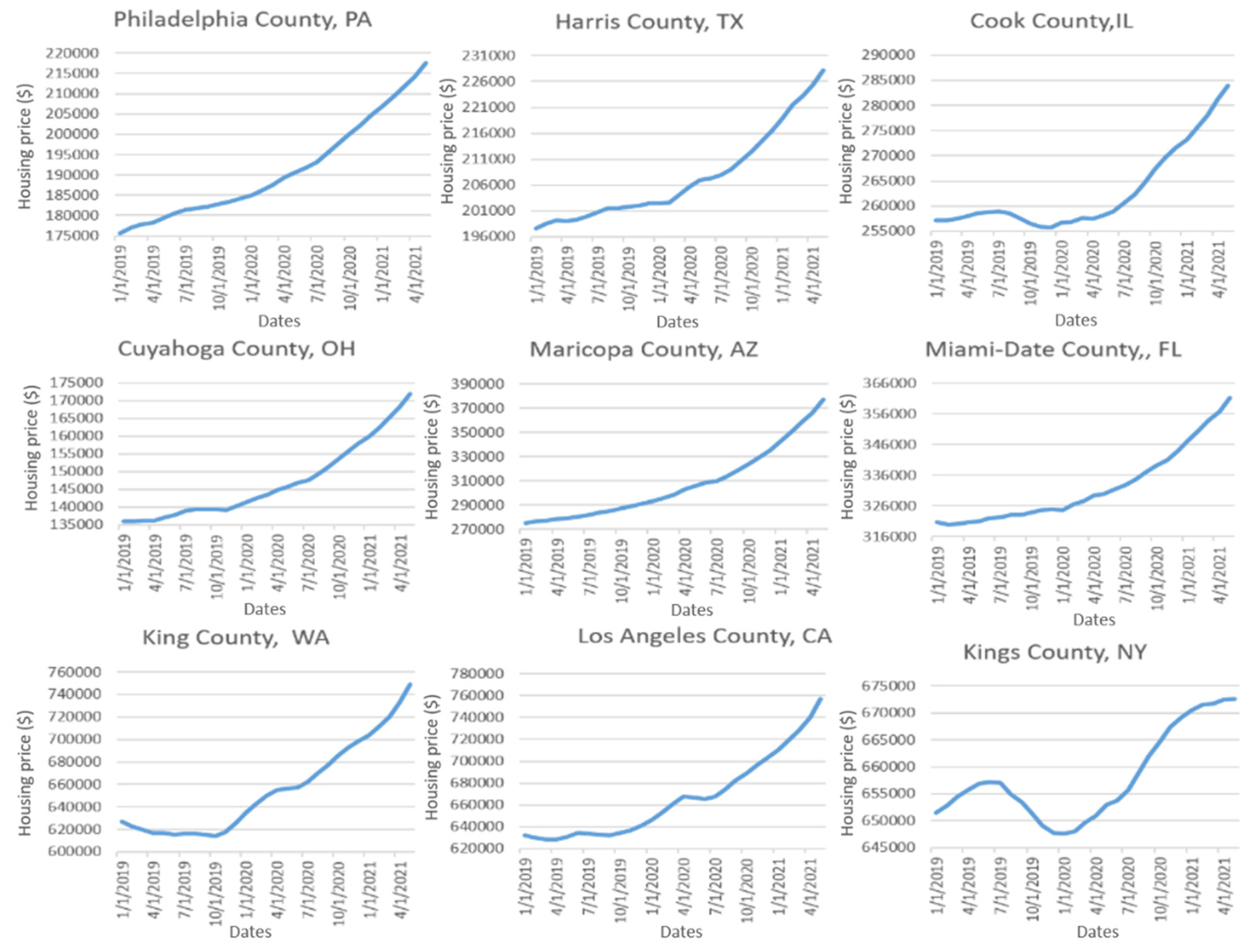
To determine whether or not the outbreak of the COVID-19 pandemic has brought some effects on housing price changes in the U.S. real estate market, we first drew the averaged housing price change trend graph based on the data of all of the U.S. counties from 1 January 2019 to 31 May 2021 in Figure 1. It can be seen that housing prices increased greatly since the start of the COVID-19 pandemic. Figure 2 shows some county examples of housing price changes from 1 January 2019 to 31 May 2021. It can be seen that while the housing prices in most U.S. counties increased steadily from 1 January 2019 to 31 May 2021, the price change patterns are not the same. Most have steady increase patterns, but some have slow-down or even dip patterns in the early stage of the COVID pandemic (April/May 2020) or right before the COVID pandemic. This suggests that the COVID-19 pandemic may have affected housing price changes differently across different counties in the U.S. real estate market.

To determine whether or not the outbreak of the COVID-19 pandemic has brought some uneven effects on housing price change in the U.S, we visualized housing price change rates across different U.S. counties during the pandemic year of 2020–2021 (from 1 May 2020 to 1 May 2021). Figure 3 shows the visualization map of housing price change rates during the pandemic year of 2020–2021. Blue colors represent the negative housing price change rates while yellow and red colors denote the positive housing price change rates. The white colors inside the maps indicate that some counties have no available housing price data. Please note that there are 252 counties without ZHVI data among the total 3108 counties. Therefore, we conducted spatial analysis and modeling for the 2856 U.S. counties having available ZHVI data, and the other 252 counties were omitted from further analysis in this study. From the maps, it can be seen that in general the housing prices dramatically increased in the majority of the U.S. counties during the pandemic year of 2020–2021. Housing prices in some counties increased by more than 30%. However, the housing prices changed unevenly across the U.S. real estate market during the pandemic year. While housing prices increased in the majority of the U.S. counties, there were still some counties having decreased housing prices. The housing prices in some counties decreased by more than 5%. We compared the housing price changes during the pandemic year of 2020–2021 with those during the nonpandemic year of 2019–2020 (from 1 May 2019 to 1 May 2020). Figure 4 shows the map of housing price change rates during the nonpandemic year of 2019–2020 using the same graduated color symbols as Figure 3. Comparing Figure 3 to Figure 4, it can be found that the housing prices increased much more in the majority of the U.S. counties during the pandemic year of 2020–2021 than during the nonpandemic year of 2019–2020. This may indicate that the COVID-19 pandemic crisis brought an effect to the U.S. real estate markets and the U.S. residential housing prices in most U.S. counties increased greatly during the pandemic crisis. To determine where the increased areas or the decreased areas were located, we overlaid the U.S. cities map with the map of housing price change rates during the pandemic year of 2020–2021, as shown in Figure 5. It can be seen that the hot spots with housing price increases mainly occurred in the areas around some of the major U.S. cities while the cold spots with housing price decreases were mainly located in some rural areas in the Midwest, Southwest, and Southeast regions.

To identify the connections between COVID-19 infection and housing price change, both OLS and GWR were used to model the association relationships between the housing price change rate variable and the explanatory variables, such as COVID-19 cases/rates, population, employment, education, poverty, and other socioeconomic variables. To find properly specified OLS models, all possible combinations of the 20 potential explanatory variables in Table 1 were evaluated using the exploratory regression tool in ArcGIS Pro. We tried setting the parameter “Minimum Number of Explanatory Variables” as 4, 5, 6, 7, 8, 9, and 10. Regardless of the minimum number of the explanatory variables required, the explanatory variable “COVID_R” or “COVID” was always among the significant explanatory variables selected for the regression models with the highest adjusted R-squared (Adj-R²) values. This indicates that the COVID-19 cases/rates variable is one of the most important explanatory variables for modeling the housing price change rates in the U.S. real estate market during the pandemic crisis. COVID-19, therefore, has obviously affected the U.S. real estate market.

Table 2. The exploratory regression output report with the highest adjusted R² results when choosing six explanatory variables for ordinary least squares (OLS) regression.

Adj-R2	AICc	JB	K(BP)	VIF	SA	Model
0.24	16,961.04	0.00	0.00	94.17	0.00	OLS Model 1: +HOUSEHOLD_SIZE *** +PER_INTERNET *** +HH_COMPUTER *** −COVID_R *** BACHELOR *** −POVALL ***
0.24	16,961.89	0.00	0.00	32.85	0.00	OLS Model 2: +PER_INTERNET *** −COVID_R *** +EMPLOYED *** −BACHELOR *** −NATURAL_IN ***
0.24	16,963.80	0.00	0.00	95.84	0.00	OLS Model 3: +HH_COMPUTER *** −COVID_R *** −BACHELOR *** +PER_BACHELOR *** −POVALL ***

Abbreviations: Adj-R²—adjusted R-squared; AICc—Akaike’s information criterion; JB—Jarque–Bera p-value; K(BP)—Koenker (BP) statistic p-value; VIF—max variance inflation factor; SA—global Moran’s I p-value; model variable sign (+/−); model variable significance (* = 0.10; ** = 0.05; *** = 0.01).

lists the exploratory regression outputs with the highest Adj-R² results when choosing six explanatory variables.

Table 3. The exploratory regression output report with the highest adjusted R² results when choosing 10 explanatory variables for OLS regression.

Adj-R2	AICc	JB	K(BP)	VIF	SA	Model
0.27	16,857.81	0.00	0.00	108.47	0.00	OLS Model 4: +HOUSELT75K *** +DP03_0024E ** +HOUSEHOLD_SIZE *** +PER_INTERNET *** +HH_COMPUTER *** −COVID_R *** −BACHELOR *** +PER_BACHELOR*** −POVALL *** −NATURAL_IN ***
0.27	16,860.68	0.00	0.00	98.43	0.00	OLS Model 5: +HOUSELT75K *** +HOUSEHOLD_SIZE *** +PER_INTERNET *** +HH_COMPUTER *** −COVID_R *** −BACHELOR *** +PER_BACHELOR *** −POVALL *** +MEDHHINC *** −NATURAL_IN ***
0.27	16,860.68	0.00	0.00	98.43	0.00	OLS Model 6: +HOUSELT75K *** +HOUSEHOLD_SIZE *** +PER_INTERNET *** +HH_COMPUTER *** −COVID_R *** +MEDIAN_HOU *** −BACHELOR *** +PER_BACHELOR *** −POVALL *** −NATURAL_IN ***

Table Abbreviations: Adj-R²—adjusted R-squared; AICc—Akaike’s information criterion; JB—Jarque–Bera p-value; K(BP)—Koenker (BP) statistic p-value; VIF—max variance inflation factor; SA—global Moran’s I p-value; model variable sign (+/−); model variable significance (* = 0.10; ** = 0.05; *** = 0.01).

lists the exploratory regression outputs with the highest Adj-R² results when choosing 10 explanatory variables. It can be seen that the explanatory variable “COVID_R” is one of the significant explanatory variables for all of the models with the highest Adj-R² values. Compared with models 1, 2, and 3 in Table 2, it can be seen that the Adj-R² of models 4, 5, and 6 in Table 3 only increased by 0.03 after four more explanatory variables were added. Considering model simplicity and increased multicollinearity problems for models 4, 5, and 6 in Table 3, the models 1, 2, and 3 in Table 2 are preferred over the models 4, 5, and 6 in Table 3. So, only the models 1, 2, and 3 in Table 2 were further evaluated in the next steps.

The small Adj-R² result (0.24) and the SA (global Moran’s I) p-value 0 for tested models 1, 2, and 3 indicate that all the models have spatially autocorrelated regression residuals and some key explanatory variables might be missed. The JB p-value of 0 for tested models 1, 2, and 3 indicates that the tested models 1, 2, and 3 are far away from having normally distributed residuals and there is model bias. This means that a key variable may be missed from the models or some of the modeled relationships are nonlinear. The K(BP) statistic p-value of 0 for the tested models 1, 2, and 3 suggests that there are nonstationarity problems in the models. This means that there are statistically significant regional variations of relationships between the dependent variable (housing price change rate here) and the explanatory variables. Because relationships between the dependent and explanatory variables are inconsistent across the study area, the computed standard errors may be artificially inflated. Therefore, using the GWR may improve the model results. Because the model with a lower AICc value designates a better-performing model, model 1 with the lowest AICc value was chosen to run OLS and GWR for further analysis.

Table 4. Summary of the OLS results with six explanatory variables.

Variable	Coefficient	StdError	t-Statistic	Probability	Robust_SE	Robust_t	Robust_Pr	VIF
Intercept	−8.457	1.287	−6.572	0.000 *	1.414	−5.981	0.000 *	-
HOUSEHOLD_SIZE	2.366	0.362	6.537	0.000 *	0.406	5.820	0.000 *	1.042
PER_INTERNET	0.172	0.011	15.001	0.000 *	0.012	14.602	0.000 *	1.235
HH_COMPUTER	0.000	0.000	13.684	0.000 *	0.000	9.683	0.000 *	94.174
COVID_R	−0.027	0.003	−8.731	0.000 *	0.003	−8.242	0.000 *	1.044
BACHELOR	−0.000	0.000	−12.869	0.000 *	0.000009	−9.345	0.000 *	38.875
POVALL	−0.000	0.000	−9.867	0.000 *	0.000	−7.108	0.000 *	21.803

* indicates a statistically significant p-value (p < 0.01).

lists the summary of the OLS results for model 1. The largest VIF value (94.17) for the explanatory variable HH_COMPUTER indicates that the variable is redundant with other explanatory variables. Removing the explanatory variable HH_COMPUTER from model 1 may solve the multicollinearity problem in model 1 and reduce the model bias or model unreliability issue. Since we only wanted to include variables that can explain a unique aspect of the housing price change rates, we chose only one of the redundant variables to be included in further analysis; thus, the explanatory variable HH_COMPUTER was removed from model 1 in further analysis.

Table 5. Summary of the OLS results with five explanatory variables.

Variable	Coefficient	StdError	t-Statistic	Probability	Robust_SE	Robust_t	Robust_Pr	VIF	StdCoef
Intercept	−11.704	1.305	−8.965	0.000*	1.459	−8.022	0.000 *	-	0
HOUSEHOLD_SIZE	2.436	0.373	6.521	0.000 *	0.414	5.889	0.000 *	1.041	0.112
PER_INTERNET	0.217	0.011	19.128	0.000 *	0.012	18.148	0.000 *	1.134	0.342
COVID_R	−0.026	0.003	−8.155	0.000 *	0.003	−7.864	0.000 *	1.043	−0.140
BACHELOR	−0.000	0.0003	−0.556	0.578	0.000	−0.440	0.660	5.655	−0.022
POVALL	0.000	0.000	3.880	0.000 *	0.000	2.400	0.016 *	5.418	0.152

* indicates a statistically significant p-value (p < 0.01).

lists the summary of the OLS results with the explanatory variable HH_COMPUTER being removed. It can be seen that the VIF values of the explanatory variables are all less than 7.5 now. This indicates that there is no serious multicollinearity problem in the model and no redundancy among the remaining explanatory variables (HOUSEHOLD_SIZE, PER_INTERNET, COVID_R, BACHELOR, POVALL) anymore. We also tested the effect of removing the explanatory variable BACHELOR instead of HH_COMPUTER. However, after BACHELOR is removed, both HH_COMPUTER and POVALL still have VIF values greater than 13.1. We, therefore, used the model with HH_COMPUTER being removed for further analysis.

For the five explanatory variables (HOUSEHOLD_SIZE, PER_INTERNET, COVID_R, BACHELOR, POVALL) used in the OLS model, each of them explains a unique aspect of the housing price change rates. The coefficient or the standardized coefficient (StdCoef) for each explanatory variable reflects both the strength and type of the relationship the explanatory variable has with the housing price change rate. The positive sign associated with the coefficients or the standardized coefficients of the explanatory variables HOUSEHOLD_SIZE, PER_INTERNET, and POVALL reflects the positive relationship between the housing price change rate and the three explanatory variables. This means that areas with larger households, higher percentages of households with Internet at home, and/or more people of all ages in poverty have larger housing price change rates. The negative coefficients or the standardized coefficient values of the explanatory variables COVID_R and BACHELOR reveal the negative relationships between the housing price change rate and these two explanatory variables. This means that areas with higher COVID rates and/or more people having bachelor degrees or higher have smaller housing price change rates. Please note that the unstandardized coefficients should not be used to compare their importance/influence in the model because the explanatory variables are measured in different units. The standardized coefficients are measured in the unit of standard deviation; therefore, they can be used to rank explanatory variables since this eliminates the units of measurement of the explanatory and dependent variables. The standardized coefficient values show that COVID_R explains about 14.0% of the housing price change rates, while PER_INTERNET explains about 34.2%, HOUSEHOLD_SIZE explains about 11.2%, POVALL explains about 15.2%, and BACHELOR explains only about 2.2%. The t test was used to assess whether an explanatory variable is statistically significant. The very small probability or robust probability (p-value) values of the four explanatory variables HOUSEHOLD_SIZE, PER_INTERNET, COVID_R, and POVALL indicate that the chance of their coefficients being essentially zero is very small, so these variables are statistically significant. This means that these explanatory variables are important to the regression model if the relationships being modeled are primarily linear and the explanatory variables are not redundant to the other explanatory variables in the model.

Table 6. Summary diagnostics of the OLS model with the five explanatory variables (HOUSEHOLD_SIZE, PER_INTERNET, COVID_R, BACHELOR, POVALL).

Diag_Name	Diag_Value
AIC	17,140.804
AICc	17,140.843
R2	0.196
Adj-R2	0.194
F-Stat	138.857
F-Prob	2.220 × 10−16 *
Wald	596.804
Wald-Prob	9.916 × 10−127 *
K(BP)	65.007
K(BP)-Prob	1.116 × 10−12 *
JB	1006.814
JB-Prob	0 *

* indicates a statistically significant p-value (p < 0.01).

lists summary diagnostics of the OLS model with the five explanatory variables (HOUSEHOLD_SIZE, PER_INTERNET, COVID_R, BACHELOR, POVALL).

The small coefficient of determination R² value indicates only 19.6% of the variation in the dependent variable (the housing price change rate variable) is explained by the OLS model. The Adj-R² value is just a bit lower than the R² value. Please note that the Adj-R² value reflects model complexity (the number of variables) as it relates to the data and is consequently a more accurate measure of model performance. The Adj-R² value of 0.194 indicates that the explanatory variables used in the linear OLS regression explain approximately 19.4% of the variation of the housing price change rates. In other words, the OLS model only tells about 19.4% of the housing price change rates. Both the joint F-statistic (F-Stat) and joint Wald statistic (Wald) are measures of overall model statistical significance. The joint F-statistic is trustworthy only when the Koenker (BP) statistic (K(BP)) is not statistically significant. Since the Koenker (BP) statistic is significant, the joint Wald statistic rather than the joint F-statistic was used to determine overall model significance. The very small p-value (probability) of the joint Wald statistic (9.916 × 10⁻¹²⁷) indicates that the OLS model is a statistically significant model. The very small K(BP) probability value (1.116 × 10⁻¹²) indicates that there is statistically significant nonstationarity in the OLS model. This means that the explanatory variables in the OLS models do not have a consistent relationship with the housing change rates across the geographic space and data space. Therefore, the OLS model with statistically significant nonstationarity may be a good candidate for GWR analysis. The JB statistic indicates whether the model residuals are normally distributed. The p-value (probability) of 0 for this test means that the residuals are not normally distributed, indicating the OLS model is biased. The bias may be the result of model misspecification (e.g., a key variable being missed from the model) when the residuals have statistically significant spatial autocorrelation. The statistically significant JB test may also occur when the OLS is used to model nonlinear relationships (e.g., the data include influential outliers or there is strong heteroscedasticity).

To determine whether or not the biased OLS model is caused by misspecification, spatial autocorrelation of the OLS regression residuals was assessed by (1) mapping the standardized residuals of the OLS results and (2) calculating the Anselin’s local Moran’s I for cluster and outlier analysis. Figure 6 shows the assessment results of the OLS residual spatial autocorrelation: the map in Figure 6a visualizes the standardized residuals, and the map in Figure 6b shows the clusters and outliers of the standardized residuals. It can be seen that the regression residuals are not spatially random (Figure 6a), and there are clear spatial clusters of high and low residuals (model underpredictions and overpredictions) (Figure 6b), which indicate the existence of significant spatial autocorrelation. The statistically significant spatial autocorrelation of the OLS regression residuals may indicate that one or more key explanatory variables are missed from the model or there are spatially heterogeneous association relationships between the housing price change rate and the explanatory variables. Therefore, the OLS results cannot be trusted.

Figure 7 shows the histogram of the OLS standardized residuals. It can be seen that the histogram span is fairly wide and there are some large positive residuals and some large negative residuals. The mean is almost zero due to the fact that the positive residuals are almost equal to the negative residuals. Figure 8 shows the scatterplot of the OLS standardized residuals. It can be seen that the scatterplot has a clear trend. This trend (nonrandom pattern) means that the OLS model does not fit well and has large room for improvement.

The statistically significant spatial autocorrelation in the OLS model residuals suggests that the OLS model is not a good model here. The OLS regression model, which is a global statistic model, probably only represents a broad spatial trend and may mask significant local variations. To deal with regional variations, GWR, which can incorporate regional variations into regression, was further explored in this study. The same explanatory variables (HOUSEHOLD_SIZE, PER_INTERNET, COVID_R, BACHELOR, POVALL) were used for GWR analysis to explore the association relationships between the housing price change rate and the five explanatory variables across the U.S. counties.

Table 7. The geographically weighted regression (GWR) model diagnostic results.

Diagnostic Names	R2	Adj-R2	AICc	σ2	σ2 MLE	Effective Degree of Freedom
Diagnostic values	0.744	0.506	17,167.570	14.476	7.490	1477.734

shows the GWR model diagnostic results.

Compared with the R² (0.196) and Adj-R² (0.194) of the OLS model (Table 6), the R² and Adj-R² of the GWR model are largely improved, with the values of 0.744 and 0.506, respectively (Table 7). The higher R² and Adj-R² values indicate that a much higher proportion of the variation of the housing price change rates is accounted for by the GWR regression model. Compared with the variance (σ²) value (23.59) of the OLS model, the smaller σ² value (14.48) of the GWR model indicates a smaller least-squares estimate of the variance for the GWR residuals. The value of the σ² MLE, a maximum likelihood estimate (MLE) of the variance of the GWR residuals, is small (7.49), which is preferable. The value of the effective degree of freedom (1477.734) reflects a tradeoff between the variance of the fitted values and the bias in the coefficient estimates, and it is related to the choice of neighborhood size, which is 6 in this study and was chosen via the trial-and-error learning method.

Figure 9 shows the spatial autocorrelation assessment results of the GWR residuals: the map in Figure 9a visualizes the standardized residuals of the GWR results, and the map in Figure 9b shows the clusters and outliers of the GWR standardized residuals based on the calculated local Moran’s I values. Comparing these mapping results with those in Figure 6, it can be seen that the GWR regression residuals are almost spatially random (Figure 9a) and there are very few clusters of high and low GWR residuals (model underprediction and overprediction) (Figure 9b). This indicates that the GWR model is much better than the OLS model and the GWR results can be trusted.

Figure 10 shows the histogram of the GWR standardized residuals. Compared with the histogram of the OLS standardized residuals (shown in Figure 7), it can be seen that the histogram of the GWR standardized residuals has a fairly narrow span and there are fewer large positive residuals and fewer large negative residuals. Most of the residuals are very small and close to 0.

Table 8. Statistics of the GWR standardized residuals.

Mean	Median	Std. Dev.	Count	Min	Max	Sum	Skewness	Kurtosis
−0.00114	−0.073	0.885	2856	−4.045	6.248	−3.257	0.771	7.333

lists some statistics of the GWR standardized residuals. The standard deviation is 0.885, which is smaller than that of the OLS standardized residuals (0.999). The small skewness value (0.77) indicates that the distribution of the GWR standardized residuals is close to the normal distribution. The value of kurtosis, 7.33, indicates a leptokurtic distribution, which produces more outliers than the normal distribution. Figure 11 shows the scatterplot of the GWR standardized residuals. Compared with the scatterplot of the OLS standardized residuals shown in Figure 8, it can be seen that the scatterplot of the GWR standardized residuals has a nearly random pattern. This nearly random pattern means that the GWR model fits quite well.

Figure 12 shows the local coefficient maps for the explanatory variables in the GWR modeling, which demonstrate the obvious spatial variation of the relationships between the housing price change rate and the five explanatory variables (HOUSEHOLD_SIZE, PER_INTERNET, COVID_R, BACHELOR, POVALL). The local coefficients for every explanatory variable change with locations from negative to positive. This indicates the spatially nonstationary relationships between the housing price change rate and the explanatory variables. Please note that the coefficient values of the variable POVALL are very small (close to zero) but are still statistically significant, which means that the variable is significant for the GWR model. Because the explanatory variables are expressed in different units, it would be unfair to compare the coefficient values of the explanatory variables to rank their contributions to the housing price change rate in the model. Although the coefficient values are not suitable here for comparison between explanatory variables, they are proper for interpreting the spatial variation of the relationships between the housing price change rate and each independent variable.

The local coefficients of the COVID-19 rate range from −0.18 to 0.13, indicating it may have negative or positive contributions to the housing price change rate in different counties, depending on the specific locations. The COVID-19 rate variable has a negative influence on the housing price change rate mainly in the densely populated areas (e.g., Los Angeles, Seattle, New York City, and Florida) and has a positive influence mainly in the sparely populated areas (e.g., Idaho, Arizona, and Maine), especially in the southeast and west regions. However, there are some exceptions; for example, the coefficients of COVID-19 rate in North Dakota (a sparely populated area) are obviously negative, but in Chicago (a densely populated area) they are almost neutral (no influence). There should be some special reasons behind the exceptions.

Local R-squared (R²) was used to explore the capability of the GWR model to fit the observation data. The high local R² values mean good performances. Figure 13 shows the local R² map of the GWR model. Obviously, the values of local R² change with spatial locations. It has a fairly small standardized deviation (0.131). The minimum local R² value is 0.048 and the maximum value is 0.94. Local R² values are higher than 0.80 in many U.S. counties. Only a very few counties have local R² values less than the R² (0.196) or Adj-R² (0.194) of the OLS model. This means that the GWR model performed much better than the OLS model for almost all of the U.S. counties.

4. Discussions and Conclusions

Although many studies have been conducted to investigate the impacts of the COVID-19 pandemic on the real estate markets in the world, the spatial dimension of such impacts is still underexplored. There seems to be no publication in the literature modeling the spatial effect of the COVID-19 pandemic on housing price changes. Focusing on spatial autocorrelation and heterogeneity, we quantitatively examined the effect of the COVID-19 pandemic on housing price changes across U.S. counties using spatial analysis and modeling methods.

In general, housing prices rose significantly across the U.S. during the COVID-19 pandemic. Housing prices increased primarily because of a surge in demand and a decrease in supply in most U.S. counties. The boom, however, was spatially heterogeneous. Some areas saw a housing price increase of more than 30%, while some other areas saw almost no increase or a decrease. Housing price changes depend largely on local conditions. This means that the impact of COVID-19 on housing price changes is not uniform across the U.S. real estate market. This result is consistent with the results of studying the impact of the global financial crisis on the housing market from a geographic perspective. For example, Li and Wei (2020) found that housing price changes after the global financial crisis differed across space and were strongly associated with the spatial distribution of local neighborhood conditions and urban amenities. Martin (2011) also found that the global financial crisis had locally varying impacts on housing markets.

To understand the factors that affected the housing price changes in the U.S. residential housing market, we first used the exploratory regression tool in ArcGIS Pro to find a properly specified OLS model for explaining housing price change rates in this study. We tested 20 explanatory variables, including the COVID-19 cases variable, the COVID-19 rate variable, and 18 other socioeconomic variables. We explored the best OLS models with different minimum numbers (4 to 10) of explanatory variables. No matter how we set up the minimum number of explanatory variables, the COVID-19 rate (or cases) variable was always among the selected significant variables for the regression models with the highest Adj-R² values. This finding suggests that housing price changes in the U.S. real estate market have a solid connection with COVID-19 characteristics during the COVID-19 pandemic.

We explored the OLS model with five explanatory variables (HOUSEHOLD_SIZE, PER_INTERNET, COVID_R, BACHELOR, POVALL) after removing the multicollinearity problem. We found that there is spatial autocorrelation in the OLS regression residuals. The spatial autocorrelation implies that the spatial distribution of the OLS regression residuals is nonrandom and the statistical independence assumption is violated in the OLS regression analysis. To explore the spatial nonstationary relationships between housing price change rate and COVID-19 factor, the GWR model, which explicitly allows parameter estimates to vary over space, was adopted in this study using the same five explanatory variables (HOUSEHOLD_SIZE, PER_INTERNET, COVID_R, BACHELOR, POVALL). We found that the explanatory variables HOUSEHOLD_SIZE, PER_INTERNET, and POVALL all have positive relationships with the housing price change rate. This means that the areas with larger households, higher percentages of households with Internet at home, and/or more people of all ages in poverty have larger housing price change rates. The explanatory variables COVID_R and BACHELOR have negative relationships with the housing price change rate. This means that the areas with higher COVID rates and/or more people having bachelor degrees or higher have smaller housing price change rates. It turns out that the GWR model is more suitable to accurately describe the spatial heterogeneity. The statistical improvement of GWR over OLS suggests that the GWR model has a better capability to characterize the spatial nonstationarity relationships between the housing price change rate and the explanatory variables, including the COVID-19 rate. The local coefficient map of the COVID-19 rate explanatory variable shows that housing price change rates are strongly associated with the spatial distribution of the COVID-19 rates. This means that the influence of COVID-19 on the U.S. real estate market is spatially imbalanced. The housing market volatility is also amplified by the uneven distributions of some socioeconomic factors, such as average household size, percent of households with Internet at home, education, and poverty variables. The GWR model has the unique advantage of visually demonstrating the spatially different association relationships between COVID-19 characteristics and housing price change rates among U.S. counties.

The uneven housing price changes may bring an uneven spillover effect to the rest of the economy and lead to divergence in economic growth across different areas. For example, the spatial difference in housing price change may result in different saving and consumption behaviors of homeowners and renters. Homeowners and renters would increase or decrease their saving and consumption based on the housing price increase or decrease in their locations. Housing market investment or construction may also behave differently because of the varying house price changes across space. In general, rising housing prices in some places may encourage consumer spending and lead to higher economic growth because of the wealth effect. On the contrary, falling housing prices in other places may negatively affect consumer confidence and housing construction and lead to lower economic growth. Via spatially uneven housing price changes, several broad economic outcomes such as income, employment, and total output may be affected differently across the different locations as a consequence. Therefore, policymakers may benefit from monitoring spatially different housing price changes in different property markets to make effective policies to fight against the COVID-19 pandemic. The findings from our study imply that governments, policymakers, and/or related businesses should consider local situations or local economic activities when they form their real estate market policies or take actions to fight recession due to the heterogeneous impacts of the COVID-19 pandemic on the housing market. In addition to the available federal programs and legislation, more effective local policies and programs should be developed to improve housing affordability by considering local situations. Local specific housing policies and programs may address the lack of housing affordability that the spatially heterogeneous U.S. communities face. Spatially homogeneous policies and programs may not be helpful for some U.S. communities with different situations.

References

1. Aalbers, Manuel. 2009. Geographies of the financial crisis. Area 41: 34–42. [Google Scholar] [CrossRef] [Green Version]
2. Ahsan, Md Moynul, and Cihan Sadak. 2021. Exploring housing market and urban densification during COVID-19 in Turkey. Journal of Urban Management 10: 218–29. [Google Scholar] [CrossRef]
3. Anselin, Luc, Anil K. Bera, Raymond Florax, and Mann J. Yoon. 1996. Simple diagnostic tests for spatial dependence. Regional Science and Urban Economics 26: 77–104. [Google Scholar] [CrossRef]
4. Anselin, Luc. 1988. Model validation in spatial econometrics: A review and evaluation of alternative approaches. International Regional Science Review 11: 279–316. [Google Scholar] [CrossRef]
5. Atkinson, Tyler, James Dolmas, Christoffer Koch, Evan F. Koenig, Karel Mertens, Anthony Murphy, and Kei-Mu Yi. 2020. Mobility and engagement following the SARS-Cov-2 outbreak. FRB of Dallas Working Paper No. 2014. Available online: https://ssrn.com/abstract=3607732 (accessed on 5 November 2021).
6. Balemi, Nadia, Roland Füss, and Alois Weigand. 2021. COVID-19′s impact on real estate markets: Review and outlook. Financial Markets and Portfolio Management 35: 495–513. [Google Scholar] [CrossRef] [PubMed]
7. Bayoumi, Tamim, and Yunhui Zhao. 2020. Incomplete Financial Markets and the Over-Development of the Chinese Housing Sector. IMF Working Paper 20/265. Available online: https://ssrn.com/abstract=3710338 (accessed on 5 November 2021).
8. Beard, Virginia. 2020. COVID-19: Poverty, Housing, Homelessness–A Broad View and a Picture from West Michigan. Available online: http://dx.doi.org/10.2139/ssrn.3613030 (accessed on 20 May 2021).
9. Bitter, Christopher, Gordon F. Mulligan, and Sandy Dallerba ’. 2007. Incorporating spatial variation in housing attribute prices: A comparison of geographically weighted regression and the spatial expansion method. Journal of Geographical Systems 9: 7–27. [Google Scholar] [CrossRef] [Green Version]
10. Blakeley, Grace. 2021. Financialization, real estate and COVID-19 in the UK. Community Development Journal 56: 79–99. [Google Scholar] [CrossRef]
11. Brunsdon, Chris A., Stewart Fotheringham, and Martin E. Charlton. 1996. Geographically weighted regression: A method for exploring spatial nonstationarity. Geographical Analysis 28: 281–98. [Google Scholar] [CrossRef]
12. Case, Karl E., John M. Quigley, and Robert J. Shiller. 2005. Comparing wealth effects: The stock market versus the housing market. Advances in Macroeconomics 5: 1–34. [Google Scholar] [CrossRef]
13. Cheung, Ka Shing, Chung Yim Yiu, and Chuyi Xiong. 2021. Housing Market in the Time of Pandemic: A Price Gradient Analysis from the COVID-19 Epicentre in China. Journal of Risk and Financial Management 14: 108. [Google Scholar] [CrossRef]
14. Chong, Terence Tai Leung, and Hengliang Liu. 2020. How Does the COVID-19 Pandemic Affect Housing Prices in China? Available online: https://mpra.ub.uni-muenchen.de/102103/1/MPRA_paper_102103.pdf (accessed on 5 August 2021).
15. Custodio, Claudia, Dragana Cvijanovic, and Moritz Wiedemann. 2021. Opioid Crisis and Real Estate Prices. CEPR Discussion Paper No. DP16272. Available online: https://repec.cepr.org/repec/cpr/ceprdp/DP16272.pdf (accessed on 20 June 2021).
16. De Toro, Pasquale, Francesca Nocca, and Francesca Buglione. 2021. Real Estate Market Responses to the COVID-19 Crisis: Which Prospects for the Metropolitan Area of Naples (Italy)? Urban Science 5: 23. [Google Scholar] [CrossRef]
17. Del Giudice, Vincenzo, Pierfrancesco De Paola, and Francesco Paolo Del Giudice. 2020. COVID-19 infects real estate markets: Short and mid-run effects on housing prices in Campania region (Italy). Social Sciences 9: 114. [Google Scholar] [CrossRef]
18. D’Lima, Walter, and Mark Thibodeau. 2022. Health crisis and housing market effects-evidence from the US opioid epidemic. The Journal of Real Estate Finance and Economics, 1–18. [Google Scholar] [CrossRef]
19. D’Lima, Walter, Luis Arturo Lopez, and Archana Pradhan. 2020. COVID-19 and Housing Market Effects: Evidence from US Shutdown Orders. Available online: https://ssrn.com/abstract=3647252 (accessed on 5 September 2021).
20. Forrest, Ray, and Ngai Ming Yip, eds. 2011. Housing Markets and the Global Financial Crisis: The Uneven Impact on Households. Cheltenham: Edward Elgar Publishing. [Google Scholar]
21. Fotheringham, A. Stewart, Chris Brunsdon, and Martin Charlton. 2003. Geographically Weighted Regression: The Analysis of Spatially Varying Relationships. Hoboken: John Wiley & Sons. [Google Scholar]
22. Francke, Marc, and Matthijs Korevaar. 2021. Housing markets in a pandemic: Evidence from historical outbreaks. Journal of Urban Economics 123: 103333. [Google Scholar] [CrossRef]
23. Goodman, Allen C. 1981. Housing submarkets within urban areas: Definitions and evidence. Journal of Regional Science 21: 175–85. [Google Scholar] [CrossRef]
24. Goodman, Allen C., and Thomas G. Thibodeau. 1998. Housing market segmentation. Journal of Housing Economics 7: 121–43. [Google Scholar] [CrossRef]
25. Goodman, Laurie, and Dan Magder. 2020. Avoiding a COVID-19 Disaster for Renters and the Housing Market. Washington, DC: Urban Institute. [Google Scholar]
26. Grimes, Arthur, and Sean Hyland. 2015. Housing markets and the global financial crisis: The complex dynamics of a credit shock. Contemporary Economic Policy 33: 315–33. [Google Scholar] [CrossRef]
27. Hamzah, Amir, Mohd Faizun Yazid, and Mohd Farid Shamsudin. 2020. Post covid-19: What next for real estate industrial sector in Malaysia? Journal of Postgraduate Current Business Research 1: 1–4. Available online: https://www.abrn.asia/ojs/index.php/jpcbr/article/download/97/79 (accessed on 10 June 2021).
28. Hoesli, Martin, and Richard Malle. 2021. Commercial real estate prices and COVID-19. Journal of European Real Estate Research. [Google Scholar] [CrossRef]
29. Hu, Maggie R., Adrian D. Lee, and Dihan Zou. 2021. COVID-19 and Housing Prices: Australian Evidence with Daily Hedonic Returns. Finance Research Letters 43: 101960. [Google Scholar] [CrossRef] [PubMed]
30. Jones, Antwan, and Diana S. Grigsby-Toussaint. 2020. Housing stability and the residential context of the COVID-19 pandemic. Cities & Health. [Google Scholar] [CrossRef]
31. Jones, Colin, and Harry W. Richardson. 2014. Housing markets and policy in the UK and the USA: A review of the differential impact of the global housing crisis. International Journal of Housing Markets and Analysis 7: 129–44. [Google Scholar] [CrossRef]
32. Kholodilin, Konstantin A. 2020. Housing Policies Worldwide during Coronavirus Crisis: Challenges and Solutions. DIW focus, No. 2. Berlin: Deutsches Institut für Wirtschaftsforschung (DIW), Available online: https://www.econstor.eu/bitstream/10419/219095/1/1697310303.pdf (accessed on 15 June 2021).
33. Kuk, John, Ariela Schachter, Jacob William Faber, and Max Besbris. 2021. The COVID-19 Pandemic and the Rental Market: Evidence from Craigslist. American Behavioral Scientist 65: 1623–48. [Google Scholar] [CrossRef]
34. Li, Han, and Yehua Dennis Wei. 2020. Spatial inequality of housing value changes since the financial crisis. Applied Geography 115: 102141. [Google Scholar] [CrossRef]
35. Li, Han, Yehua Dennis Wei, Zhou Yu, and Guang Tian. 2016. Amenity, accessibility and housing values in metropolitan USA: A study of Salt Lake County, Utah. Cities 59: 113–25. [Google Scholar] [CrossRef]
36. Li, Xinba, and Chuanrong Zhang. 2021. Did the COVID-19 Pandemic Crisis Affect Housing Prices Evenly in the US? Sustainability 13: 12277. [Google Scholar] [CrossRef]
37. Ling, David C., Chongyu Wang, and Tingyu Zhou. 2020. A first look at the impact of COVID-19 on commercial real estate prices: Asset-level evidence. The Review of Asset Pricing Studies 10: 669–704. [Google Scholar] [CrossRef]
38. Liu, Sitian, and Yichen Su. 2021. The impact of the COVID-19 pandemic on the demand for density: Evidence from the US housing market. Economics Letters 207: 110010. [Google Scholar] [CrossRef]
39. Lu, Binbin, Martin Charlton, Paul Harris, and A. Stewart Fotheringham. 2014. Geographically weighted regression with a non-Euclidean distance metric: A case study using hedonic house price data. International Journal of Geographical Information Science 28: 660–81. [Google Scholar] [CrossRef]
40. Maclennan, Duncan, and Anthony O’Sullivan. 2011. The global financial crisis: Challenges for housing research and policies. Journal of Housing and the Built Environment 26: 375–84. [Google Scholar] [CrossRef]
41. Marona, Bartłomiej, and Mateusz Tomal. 2020. The COVID-19 pandemic impact upon housing brokers’ workflow and their clients’ attitude: Real estate market in Krakow. Entrepreneurial Business and Economics Review 8: 221–32. [Google Scholar] [CrossRef]
42. Martin, Ron. 2011. The local geographies of the financial crisis: From the housing bubble to economic recession and beyond. Journal of Economic Geography 11: 587–618. [Google Scholar] [CrossRef] [Green Version]
43. Miller, Norman, Liang Peng, and Michael Sklarz. 2011a. The economic impact of anticipated house price changes—Evidence from home sales. Real Estate Economics 39: 345–78. [Google Scholar] [CrossRef]
44. Miller, Norman, Liang Peng, and Michael Sklarz. 2011b. House prices and economic growth. The Journal of Real Estate Finance and Economics 42: 522–41. [Google Scholar] [CrossRef]
45. Murphy, Laurence. 2011. The global financial crisis and the Australian and New Zealand housing markets. Journal of Housing and the Built Environment 26: 335–51. [Google Scholar] [CrossRef]
46. Nicola, Maria, Zaid Alsafi, Catrin Sohrabi, Ahmed Kerwan, Ahmed Al-Jabir, Christos Iosifidis, Maliha Agha, and Riaz Agha. 2020. The socio-economic implications of the coronavirus pandemic (COVID-19): A review. International Journal of Surgery 78: 185–93. [Google Scholar] [CrossRef]
47. Qian, Xianhang, Shanyun Qiu, and Guangli Zhang. 2021. The impact of COVID-19 on housing price: Evidence from China. Finance Research Letters 43: 101944. [Google Scholar] [CrossRef]
48. Ramani, Arjun, and Nick Bloom. 2021. The donut effect: How COVID-19 shapes real estate. SIEPR Policy Brief. Available online: https://siepr.stanford.edu/publications/policy-brief/donut-effect-how-covid-19-shapes-real-estate (accessed on 10 June 2021).
49. Tanrıvermiş, Harun. 2020. Possible impacts of COVID-19 outbreak on real estate sector and possible changes to adopt: A situation analysis and general assessment on Turkish perspective. Journal of Urban Management 9: 263–69. [Google Scholar] [CrossRef]
50. Tyndall, Justin. 2019. Getting high and low prices: Marijuana dispensaries and home values. Real Estate Economics 49: 1093–119. [Google Scholar] [CrossRef]
51. Uchehara, Ikechukwu, Mansur Hamma-Adama, Kwadwo Ayeh Obiri, Naeimeh Jafarifar, and David Moore. 2020. Impacts and risk management of COVID-19 pandemic on real estate supply chain. International Journal of Real Estate Studies 14: 41–53. [Google Scholar]
52. Verhaeghe, Pieter-Paul, and Abel Ghekiere. 2021. The impact of the COVID-19 pandemic on ethnic discrimination on the housing market. European Societies 23: S384–S99. [Google Scholar] [CrossRef]
53. Wang, Bingbing. 2021. How Does COVID-19 Affect House Prices? A Cross-City Analysis. Journal of Risk and Financial Management 14: 47. [Google Scholar] [CrossRef]
54. Wong, Grace. 2008. Has SARS infected the property market? Evidence from Hong Kong. Journal of Urban Economics 63: 74–95. [Google Scholar] [CrossRef] [PubMed]
55. Yilmazkuday, Hakan. 2020. COVID-19 and Housing Prices: Evidence from US County-Level Data. Available online: https://ssrn.com/abstract=3746552 (accessed on 15 November 2021).
56. Yoruk, Baris. 2020. Early Effects of the COVID-19 Pandemic on Housing Market in the United States. Available online: https://papers.ssrn.com/sol3/papers.cfm?abstract_id=3607265 (accessed on 1 June 2021).
57. Yu, Danlin, Yehua Dennis Wei, and Changshan Wu. 2007. Modeling spatial dimensions of housing prices in Milwaukee, WI. Environment and Planning B: Planning and Design 34: 1085–102. [Google Scholar] [CrossRef]
58. Zhao, Yunhui. 2020. US Housing Market during COVID-19: Aggregate and Distributional Evidence. Washington, DC: International Monetary Fund. [Google Scholar]
59. Zillow Research. 2021. ZHVI User Guide. Available online: https://www.zillow.com/research/zhvi-user-guide/ (accessed on 10 August 2021).
Figure 1. Averaged housing price changes from 1 January 2019 to 31 May 2021.
Jrfm 15 00139 g001
Figure 2. Examples of housing price changes from 1 January 2019 to 31 May 2021.
Jrfm 15 00139 g002
Figure 3. Housing price change rates during the pandemic year of 2020–2021 (from 1 May 2020 to 1 May 2021).
Jrfm 15 00139 g003
Figure 4. Housing price change rates during the nonpandemic year of 2019–2020 (from 1 May 2019 to 1 May 2020).
Jrfm 15 00139 g004
Figure 5. Overlay of cities with housing price change rates during the pandemic year of 2020–2021.
Jrfm 15 00139 g005
Figure 6. Spatial autocorrelation assessment results of the ordinary least squares (OLS) residuals. (a) Standardized residuals of the OLS results; (b) clusters and outliers of the OLS standardized residuals.
Jrfm 15 00139 g006
Figure 7. Histogram of the OLS standardized residuals.
Jrfm 15 00139 g007
Figure 8. Scatterplot of the OLS standardized residuals.
Jrfm 15 00139 g008
Figure 9. Spatial autocorrelation assessment results of the geographically weighted regression (GWR) residuals. (a) Standardized residuals of the GWR results; (b) clusters and outliers of the GWR standardized residuals.
Jrfm 15 00139 g009
Figure 10. Histogram of the GWR standardized residuals.
Jrfm 15 00139 g010
Figure 11. Scatterplot of the GWR standardized residuals.
Jrfm 15 00139 g011
Figure 12. Local coefficient maps for explanatory variables in the GWR model.
Jrfm 15 00139 g012
Figure 13. Local R2 map of the GWR model.
Jrfm 15 00139 g013