Copula Modelling to Analyse Financial Data

Abstract

Copula modelling is a popular tool in analysing the dependencies between variables. Copula modelling allows the investigation of tail dependencies, which is of particular interest in risk and survival applications. Copula modelling is also of specific interest to economic and financial modelling as it can help in the prediction of financial contagion and periods of “boom” or “bust”. Bivariate copula modelling has a rich variety of copulas that may be chosen to represent the modelled dataset dependencies and possible extreme events that may lie within the dataset tails. Financial copula modelling tends to diverge as this richness of copula types within the literature may not be well realised with the two different types of modelling, one being non-time-series and the other being time-series, being undertaken differently. This paper investigates standard copula modelling and financial copula modelling and shows why the modelling strategies in using time-series and non-time-series copula modelling is undertaken using different methods. This difference, apart from the issues surrounding the time-series component, is mostly due to standard copula modelling having the ability to use empirical CDFs for the probability integral transformation. Financial time-series copula modelling uses pseudo-CDFs due to the standardized time-series residuals being centred around zero. The standardized residuals inhibit the estimation of the possible distributions required for constructing the copula model in the usual manner.

1. Introduction

In investigating copula modelling, it is often stated within the literature that the Gaussian (Normal) copula is to blame for the financial crash of 2007 and 2008. This general statement is a bit of an oddity, as copula modelling can be a virtually automated process. It can be a semi-automated, or even a totally manual process, based on goodness of fit estimates in copula selection. Which method is used is up to the modeller by following a copula modelling process. Blame is squarely put in using the Gaussian copula, see Salmon (2009), by financial traders in selling vast quantities of new securities and expanding financial markets to unimaginable levels. Zimmer (2012) highlights that the Gaussian copula’s inability to account for tail dependence limits its use in estimating relationships in housing price movements that can lead to model miss-specification, which is what happened in the financial crash of 2007 and 2008.

However, the problem is not with using the Gaussian copula, just with the modellers for not using a properly specified copula model, see Salmon (2009). A properly specified model may have resulted in another copula shape apart from the Gaussian copula. It is interesting to think how a totally wrong copula model can be selected that does not represent the datasets dependencies when a copula model can be generated quickly and easily with just a few lines of code, with many examples to follow within the literature.

Parametric copula modelling can be undertaken following a clear process, from identifying and determining the model’s distributions, transforming the distributions to marginal distributions (usually uniform), through to copula selection. This process is widely used and recommended, see Hofert et al. (2018) and Vuolo (2017), with other examples scattered throughout the copula modelling literature.

Upon investigating copula modelling using financial data that contain a time-series component, even though non-time-series copula and time-series copula modelling are based on the same underlying theorem, Sklar’s Theorem, Section 3, different modelling strategies must be employed. These differences are that the time-series and the volatility of the time-series data must be modelled separately before copula modelling methods can be used, see Patton (2012) and Zhang and Singh (2019). It is this time-series and volatile nature of financial data that makes copula modelling more challenging compared to the standard copula modelling process.

Financial copula modelling, should it contain a time-series component, needs to have the time-series and possible volatility parameters estimated. Then, the copula model can only be undertaken using a pseudo-CDF. Standard non-time-series copula modelling can be undertaken using either an empirical CDF or pseudo-CDF for the estimation of the marginal distributions, see Hofert et al. (2018). Using an empirical CDF for the probability integral transformation allows for determining outliers, influential data points and insight on how well the distributions fit the modelled dataset. Using an empirical CDF allows for the copula model to be estimated using actual observations, not the pseudo-observations generated from a pseudo-CDF.

Standard, non-time-series copula models consist of a rich variety of copula types, see Stamatatou et al. (2018). Popular copula model types include, but are not limited to, Gaussian, Student-t, Clayton, Frank, Gumbel, Joe and an assortment of BB copula models, see Schepsmeier et al. (2015). The variety of these copula models allows for the modelling of no tail dependence, some tail dependence or even extreme tail dependence in either survival or risk modelling Hofert et al. (2018). This also allows for a range of available copula models that can be chosen to suit the dependence structure of the modelled data, allowing for the correct model specification.

The aim of this paper is to highlight the difference between time-series copula modelling and non-time-series copula modelling and where the modelling methods diverge and why. In addition, we use the rich diversity of possible copula models Schepsmeier et al. (2015) using time-series data, such as financial data—as the literature is limited mostly focused on the common Gaussian, Gumbel, Clayton, Frank and Joe type copula models.

We proceed as follows: Section 2 introduces the background in financial copula modelling; Section 3 is copula theory; Section 4, an overview of time-series modelling; Section 5, a worked example of a financial copula model; Section 6, a brief discussion about financial copula modelling; and Section 7, makes our conclusions.

2. Background in Financial Copula Modelling

The financial crisis and subsequent worldwide economic and financial developments have made clear the importance of the analysis of financial data, see Guharay et al. (2013). Research in financial economics has been centred on modelling and simulation, both to gain insight into mechanisms of events (e.g., such as bubbles or crashes) and to characterise the system’s stability Guharay et al. (2013).

Within economics and finance, there is a particular difficulty in copula modelling Fermanian (2017) due to the time-dependence; significant advances have been observed in terms of copula modelling of univariate and multivariate time-series. Although advances have been made, financial copula modelling can be awkward as there are many different modelling strategies and using a defined process can be difficult.

The dependence of financial markets during a period of extreme fluctuations has received considerable attention within the literature, see Mensah and Adam (2020). The copula co-movements capture how shocks in a specific market may transcend to other currency markets. Therefore, measuring the co-movements and tail dependence structures and determining the volatility spill-over and evolution over time is essential in risk management, diversification and pricing, see Mensah and Adam (2020).

When modelling financial data that contain time-series, the serial correlations within the time-series play a fundamental role in the statistical process. The observed data may not be independent since the present conditions rely on the past. Appropriate models for serial correlation dependence are necessary Emura et al. (2017). Financial institutions and investors are concerned about volatility and global currency markets, which can dominate the stock and bond markets, see Mensah and Adam (2020). Copula models that contain time-series have been employed extensively to study the co-movement and tail dependence structure of financial data.

Overall, copula modelling has shown to be a worthy tool in analysing highly dependent phenomena Gródek-Szostak et al. (2019), such as financial market performance, market confidence, market speculation, drought, floods, fire, rainfall or even crop oversupply, to name a few. Overall, studies have found Bhatti and Do (2019) that copula models are good at characterising joint dependence among variables, especially when extreme values are clearly evident. Nevertheless, copula modelling is sometimes used in a “black box” fashion Haugh (2016).

Copulas allow the compounding of joint distributions when only marginal distributions are known with certainty. An important advantage is that they allow marginal distributions from different families, such as the Elliptical and Archimedean distributions Kayalar et al. (2017). Copulas also provide a flexible methodology for understanding associations between related phenomena and their joint probabilities. The copula models ask a fundamentally different question than typical techniques modelling conditional values. Rather than how does variable X influence variable Y, copulas ask, “How do two variables move together in unison and how strong is that con-current movement at various points in the distribution” Vuolo (2017).

Copula modelling can be undertaken to explore extreme events, with the main advantage of extreme value copulas Gródek-Szostak et al. (2019) being the possibility of analysing above-average losses or profits in the fields of finance and insurance, but also in the case of examining future agricultural products. Although there is an array of divergent definitions that can cause ambiguity when it comes to the definition of extreme events, see Broska et al. (2020), in the context of finance and insurance, extreme events relate to unexpected, abnormal or extreme outcomes. Common extreme value and survival copulas are the Student-t, Clayton, Galambos and BB8 (Joe-Frank) copulas.

Financial copula modelling is about identifying the time-series within the data, and there are standard families of multivariate models for financial time series. These models are the GARCH-type and/or stochastic volatility type models Fermanian (2017), and there is a dominant use of GARCH models Mensah and Adam (2020). Econometric literature contains a preponderance of evidence that the conditional volatility of economic time-series changes through time, see Patton (2012).

3. Copula Theory

The basic definition of a bivariate copula Beare (2010) is a bivariate probability distribution function on ${[0,1]}^2$ for which the two univariate marginal distribution functions are uniform on $[0,1]$. Suppose that X and Y are real-valued random variables with joint distribution function $F_{(X,Y)}$ and marginal distribution functions $F_X$ and $F_Y$. We say that X and Y admit the copula C if $C(F_X\left(x\right)$, $F_Y\left(y\right))=F_{(}X,Y)(x,y)$ for all $x,y\in R$.

Further to the above, suppose that X and Y are real-valued random variables with joint distribution function $F_{(X,Y)}$ and marginal distribution functions $F_X$ and $F_Y$. We say we can construct a copula $C(F_X\left(x\right),F_Y\left(y\right))=F(X,Y)(x,y)$ for all $x,y\in R$ if and only if the Fréchet–Hoffding bounds hold true.

Sklar’s theorem ensures that for any random variable X and Y, there exists a copula C such that X and Y admit C Beare (2010). Moreover, C is uniquely defined on the product of the ranges of the marginal distribution functions of X and Y. Hence, C is unique if X and Y are continuous random variables. If X or Y is not continuous, C may nevertheless be uniquely defined by bilinear interpolation between uniquely defined values. The practical implication of Sklar’s theorem is that modelling of the marginal distributions can be conveniently separated from the dependence modelling in terms of the copula Brechmann and Schepsmeier (2013).

Based on the Sklar’s Theorem, the copula is a mathematical function, see Li et al. (2018), of univariate marginal distribution functions for constructing the joint distribution. For a bivariate case, if the marginal distribution function of the continuous random vectors $(X,Y)$ are $F_x$ and $F_y$, the joint probability distribution function can be expressed as:

$$\begin{array}{c}\hfill P(X\le x,Y\le y)=C[F_x\left(x\right),F_y\left(y\right);\theta ]=C(u_1,u_2)\end{array}$$

(1)

where C is a copula, $\theta$ is the copula parameter that summarizes the dependence structure and $u_1=F_x\left(x\right)$, $u_2=F_y\left(y\right)$ are marginal probabilities, x and y are the realizations of X and Y. Copulas are functions Haugh (2016) that enable the separation of the marginal distributions from the dependency structure of a given multivariate distribution.

Sklar’s Theorem (1959)

Theorem 1

(Sklar’s Theorem). For any d-dimensional $dfH$ with univariate margins $F_1,\dots ,F_d$, there exists a d-dimensional copula C such that:

$$\begin{array}{c}\hfill H\left(x\right)=C(F_1\left(x_1\right),\dots ,F_d\left(x_d\right)),x\in R\end{array}$$

(2)

The complete Sklar’s theorem and proof of the theorem can be found throughout the literature. A proportion is provided there to highlight some of the important parts of the theorem. According to Sklar’s theorem (1959), for any joint distribution $F(y_1,y_2)$ with marginal cumulative distributions $F_1\left(y_1\right)$ and $F_2\left(y_2\right)$ there exists a copula function:

$$\begin{array}{c}\hfill F(y_1,y_2)=C_{\theta }(F_1\left(y_1\right),F\left(y\right))\end{array}$$

(3)

An important aspect of Sklar’s theorem is that the joint distribution of any two outcomes $y_1$ and $y_2$ can be expressed as a copula function that is determined by the individual marginal CDFs $F_1\left(y_1\right)$ and $F_2\left(y_2\right)$ and an association parameter $\theta$ that binds them together Vuolo (2017). Given that CDFs are bound between 0 and 1, by definition, the function takes a value on the square and product value on the unit value. For any two continuous marginals, the CDF is uniform from 0 to 1, or $F_1,F_2\sim U(0,1)$.

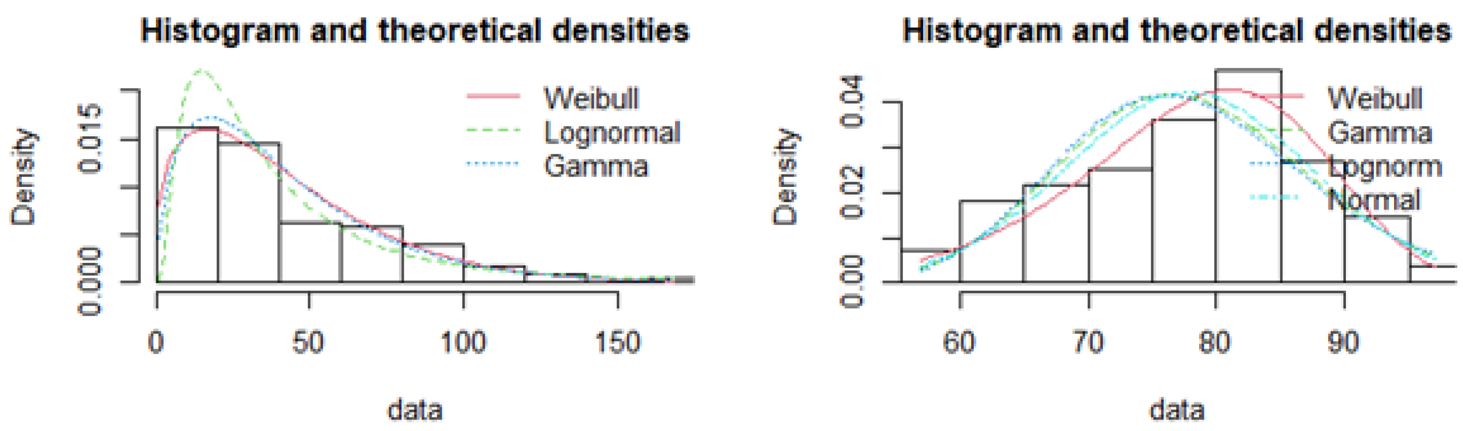
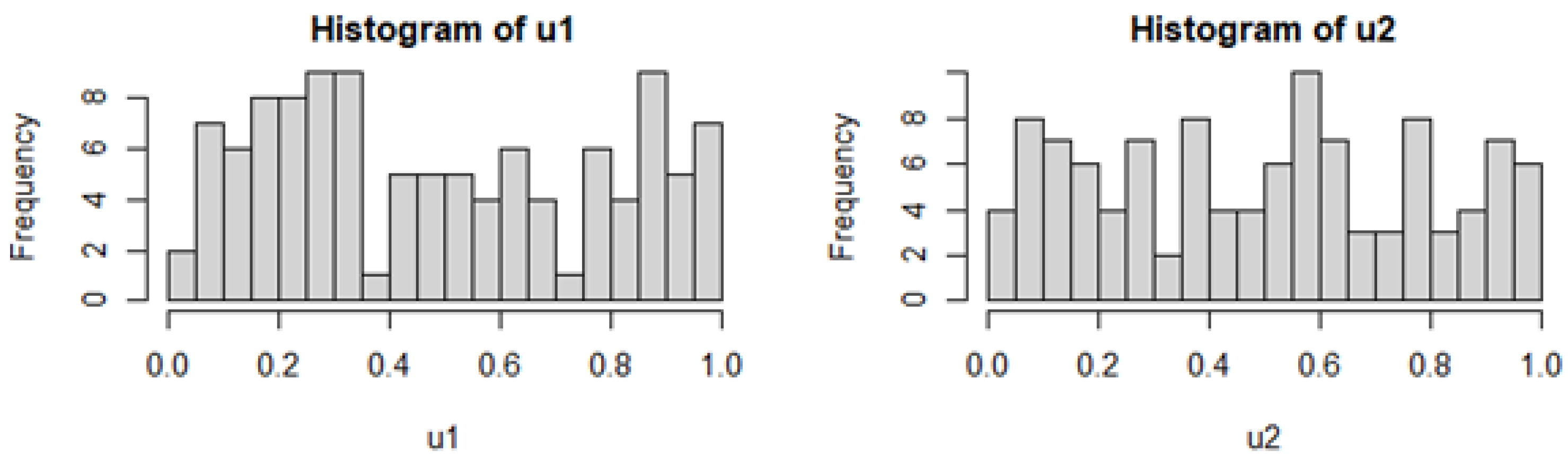
A transformation on the dataset to make the standard uniform margins is a probability transformation. Figure 1, as an example, shows the distributions that may be suited for a probability integral transformation to obtain the empirical CDFs. Figure 2 shows the uniform distribution generated from the chosen distributions by a probability integral transformation.

Although the probability integral transformation usually transforms the distributions to uniform marginal distributions, other distributions can be used, as long they are the same type of distributions Vuolo (2017)—either two uniform or two normal distributions, for example.

This is a common method in copula modelling in the absence of time-series. Financial copula modelling diverges from standard bivariate copula modelling in obtaining the uniform marginal distributions due to the time-series component, and we proceed as follows.

4. Time Series Modelling

Time-series can be defined Li et al. (2020) as a sequence of observations on one or more variables over time. Time is an important dimension because past events can influence future events. The two main features of time-series Li et al. (2020) are the data frequency and autocorrelation (the correlation between the observations of the same variable over successive time intervals). These features must be carefully modelled to allow for correctly specified residuals to be used within the copula model.

Time series modelling with no volatility can be undertaken using ARMA and ARIMA methods. The ARIMA equation is where the stationary time series is linear, in which the predictors consist of lags of the dependent variable. A nonseasonal ARIMA model is classified as am ARIMA$(p,d,q)$ model, where p is the number of autoregressive terms, d is the number of nonseasonal differences needed for stationarity, and q is the number of lagged forecast errors in the prediction equation.

The difference between an ARMA and the ARIMA is the number of needed differences in a series of observations to achieve stationarity. ARMA$(p,q)$ is equivalent to ARIMA$(p,0,q)$ and if $d>0$, an ARMA$(p,q)$ can be used after the differencing of the original time-series has achieved stationarity.

Time-series may be identified by using sample autocorrelation (ACF) and partial autocorrelation (PACF) functions for time-series, $X_t:t=1,\dots ,n$. If the sample ACF falls into the 95% confidence bound quickly, then the time series $X_t$ may be considered stationary. Otherwise, the time series is non-stationary and differencing is required to convert it to a stationary time series, see Zhang and Singh (2019).

Time-series modelling can also include ARCH and GARCH methods when there is the presents of volatility within the data. ARCH models are an AR model with conditional heteroscedasticity. If the volatility does not necessarily happen at particular times, the variance itself can be modelled with an AR(p) model. A GARCH (generalized ARCH) model is a better fit for modeling time-series data when the data exhibits heteroscedasticity and also volatility clustering.

The ARMA-GARCH time series models, model the time-series along with the volatility contained within the data. The ARMA-GARCH models are used to remove the serial correlations and conditional heteroscedasticity, see Albulescu et al. (2020).

5. Financial Copula Modelling

Financial copula modelling includes a time-dependent sequence, see Zhang and Singh (2019). The copula modelling process must account for each variables’ univariate time-series structure. The model’s residuals must be estimated from the fitted univariate time-series model and then applied to the copula to model using standardized residuals.

Financial copula modelling uses pseudo-CDFs due to the standardized residuals being centred around zero, with the fitting of gamma or lognormal distributions, as an example, to undertake the probability integral transformation not being possible. The pseudo-observations from the standardized residuals by way of a pseudo-CDF is used.

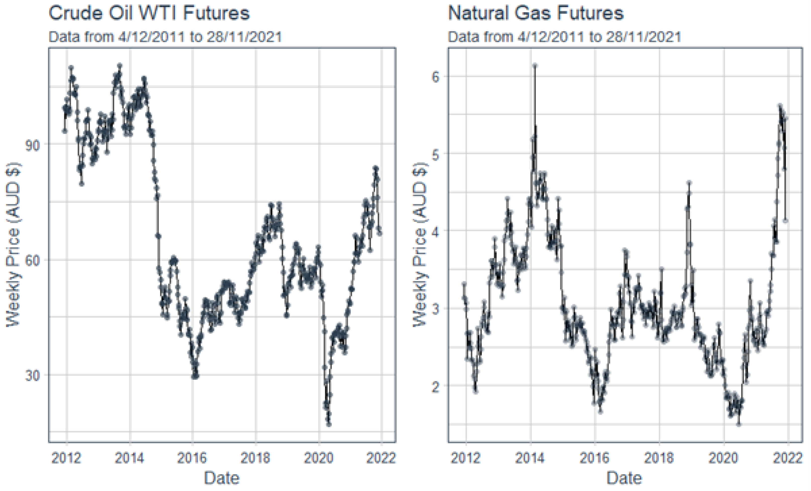
Figure 3 shows the Australian Crude Oil WTI and Natural Gas weekly Futures prices between the dates of 4 December 2012 and 28 November 2021. As an example, these time-series datasets will be used to undertake a copula model, in highlighting the copula modelling process for financial data that contains time-series.

The first steps in undertaking a financial copula modelling are determining the ARMA model, then determining the GARCH component of the time-series, or if the GARCH component is required. Once these have been obtained, the standardized residuals can be modelled into a copula. This is the most critical part of the copula modelling process, as determining the correct time-series model will allow for correct tail dependence to be modelled by way of the standardized residuals.

Literature for copula time-series modelling using ARIMA-type models can be sparse, whereas, the literature for copula time-series modelling using ARMA-GARCH models is far more abundant Mensah and Adam (2020), as the ARMA or ARMA-GARCH process models the volatility within the dataset, making them suitable for financial data. Testing whether an ARMA or ARMA-GARCH model is appropriate should be undertaken. For short time periods, an ARIMA may be appropriate, and a long time period may require the ARMA-GARCH model.

Estimating the ARIMA and ARMA parameters for Crude Oil and Natural Gas was undertaken using the auto.arima package within R software, https://CRAN.R-project.org/ (accessed on 10 April 2020), see Hyndman et al. (2020). This gave the results for Crude Oil an ARIMA model of order (2,1,1) and Natural Gas as an ARIMA model (1,1,1). After differencing, the ARMA estimated model for Crude Oil was of order (2,1) and Natural Gas was (1,1). These values and the differenced data were used for the GARCH modelling.

Fitting a GARCH model to the data was used by the ugarchfit package within the R software, https://CRAN.R-project.org/ (accessed on 10 April 2020), see Ghalanos (2020). GARCH modelling for both Crude Oil and Natural Gas gave a GARCH model result of (1,1). Using the GARCH, ugarchfit package, allowed for the fitting of the ARMA parameters for the Crude Oil and the Natural Gas datasets and the obtained residuals were then standardized.

Both datasets contained heteroscedasticity, therefore a GARCH process was used to model the volatility. The residuals conditional variance equation for Crude Oil was an ARMA(2,1)-GARCH(1,1), and Natural Gas was an ARMA(1,1)-GARCH(1,1). The ARMA-GARCH modelled the non-constant variance of the two datasets, which will produce residuals $N\approx (0,1)$. These models are used within the rest of the paper.

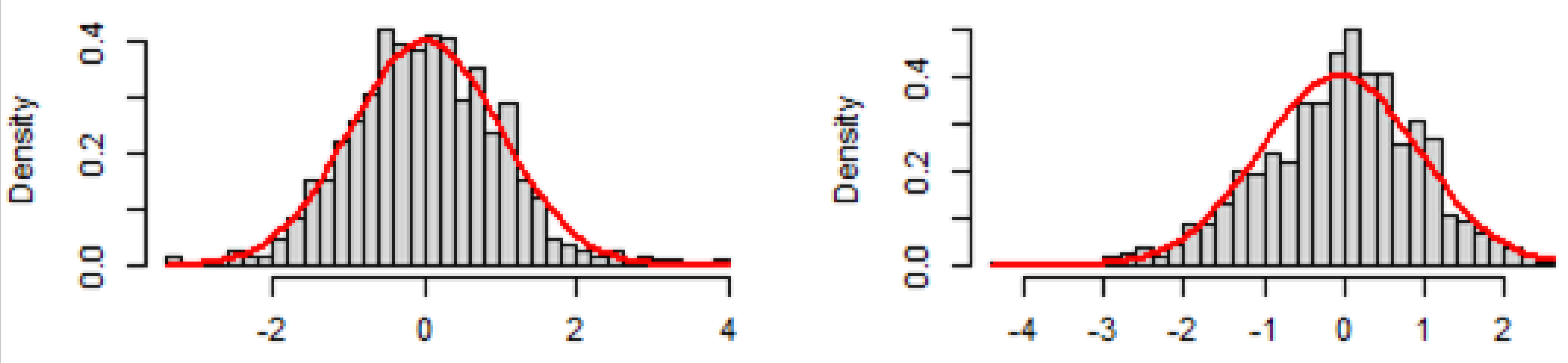
Figure 4, shows the histograms of the standardized residuals from the time-series modelling results, which are overlaid with the normal distribution. The results show that the x-axis values contain negative values. Estimation of log-normal and gamma distributions that may better fit the residuals cannot be undertaken to estimate the copulas marginal distributions. This highlights the need for copula time-series models to be based on pseudo-CDFs.

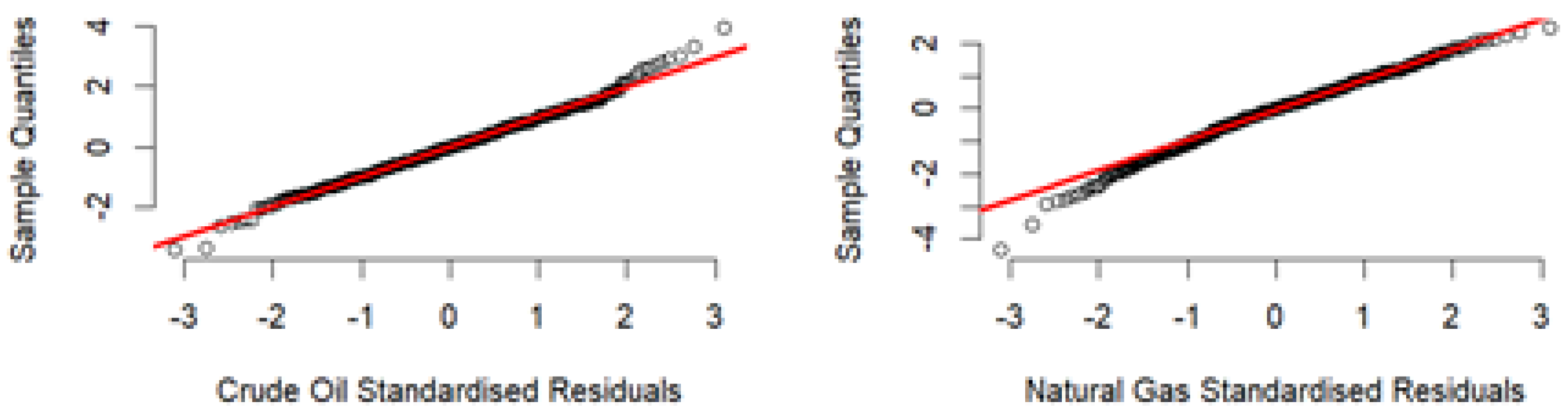
A graphical method to determine if any tail dependence is present can be represented in a Q-Q plot of the two standardized residuals for crude oil and natural gas. The Q-Q plots give an indication if the tails are not Gaussian, indicating possible tail dependence. The Q-Q plots have been plotted and shown in Figure 5. Overall, the standardized residuals for both datasets follow the Gaussian distribution, with the exemption that only a few points at the tails fall outside a Gaussian distributions.

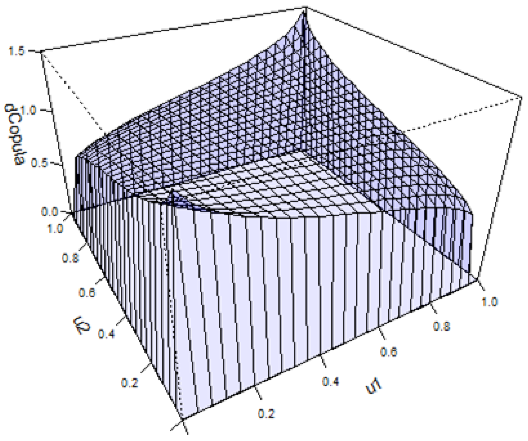
The standardized residuals were then applied to the BiCopSelect function, see Schepsmeier et al. (2015), with R software package, https://CRAN.R-project.org/ (accessed on 10 April 2020), to generate (estimate) the copula type and parameters. Figure 6, shows the results, which produced a Gaussian (Normal) copula with a $\tau$ value of 0.15. The $\tau$ value of only 0.15, which is a measure of dependence, a Pearson’s linear correlation coefficient, shows that there is very little dependence between the crude oil and natural gas prices.

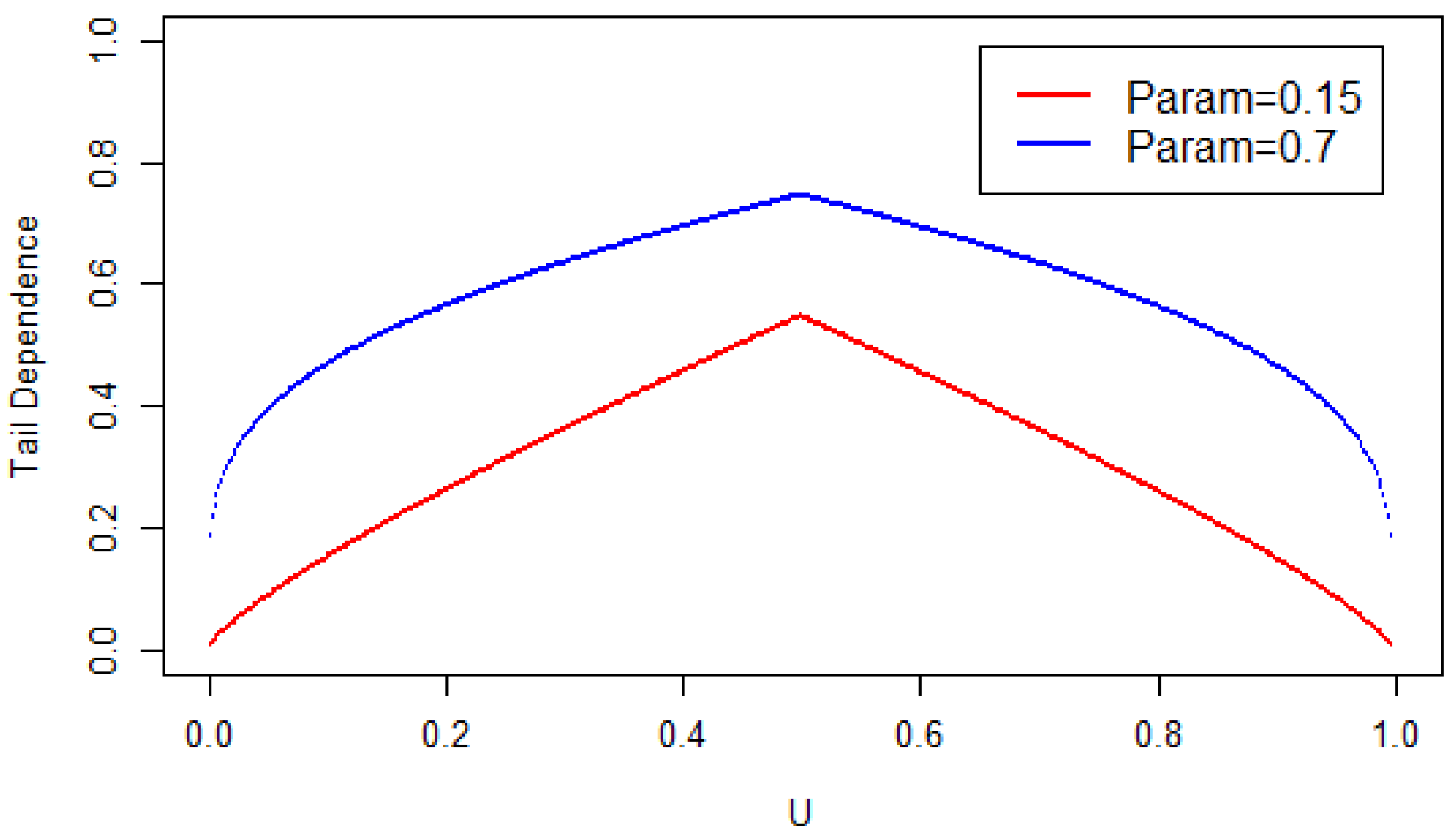
Figure 6, shows the estimated Gaussian copula which had a $\tau$ value of 0.15, with Figure 7 being included to show the Gaussian copula dependence with a $\tau$ value of 0.15 and a $\tau$ value of 0.7, which is considered a strong association value. A worthwhile endeavour in any copula modelling situation is to plot the copulas dependence. The estimated copula with the $\tau$ value = 0.15, shows significantly less dependence with no tail dependence.

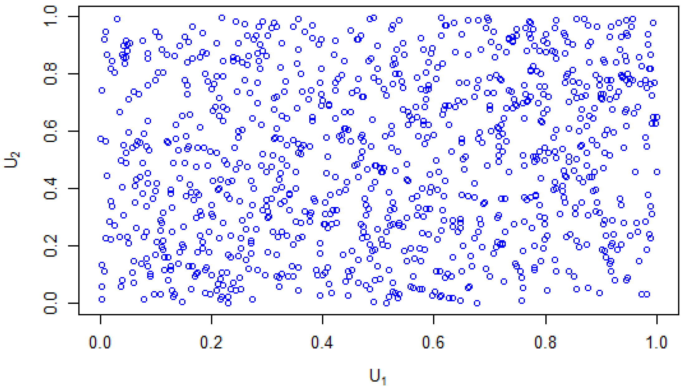
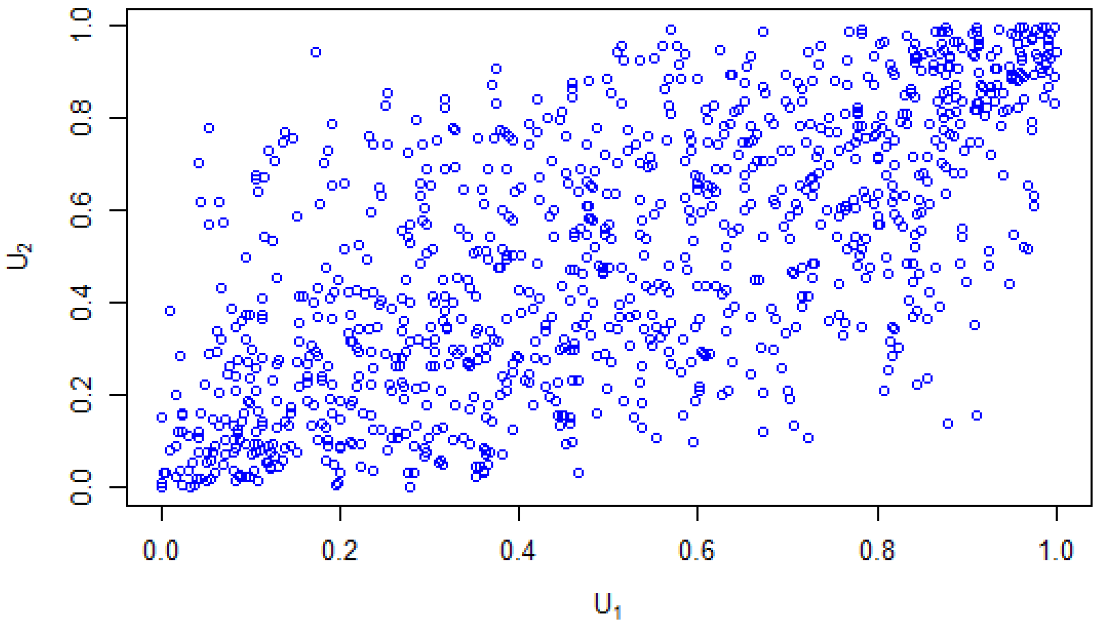
Figure 8 and Figure 9 show the comparison between the estimated Gaussian distribution of $\tau$ = 0.15, to a strong dependence value of $\tau$ = 0.7. In Figure 8, the generated copula distribution, shows a distribution that almost represents an independent copula, being that u1 and u2, are almost independent with a $\tau$ = 0.15. Figure 9, shows a distribution with another set of u1 and u2 values, having a strong dependency value of $\tau$ $=0.7$.

Therefore, we can conclude there was no dependence between the crude oil and natural gas prices, as the estimated Gaussian copula had a $\tau =0.15$. Figure 8, confirms this, as the estimated copula model represents an independent copula distribution, see Hofert et al. (2018).

6. Discussion

In returning to the original statement that the Gaussian copula can be blamed for the 2007-2008 financial crisis, Section 1, can be appreciated now. An easy approach was undertaken by the financial traders in using a Gaussian copula model Zimmer (2012), which inhibited any ability for tail dependence to be modelled and identified. This allowed for missed opportunities in detecting the “up and coming” financial bust of 2007 and 2008.

With standard copula modelling, choices can be made to use CDFs or pseudo-CDFs to model the copula. Using CDFs has the advantage of the copula model being modelled using distributions with the actual values from a dataset. Undertaking the inverse probability integral transformation using a CDF highlights potential issues within the dataset that may allow for further exploration. Smaller datasets will benefit from using a CDF, as the CDF and pseudo-CDF converge with large datasets.

Financial copula modelling requires the added process of extracting the standardised residuals from a time-series model that will allow for a financial copula model to be modelled. Unifying the time-series component and copula modelling process can be an awkward process, as there are many different modelling methods and coding options available and little guidance within the literature in having these working together coherently.

This paper has highlighted the importance of the time-series parameters to be correctly specified that will allow for the standardized residuals to be used within the copula model that will allow for a correctly-specified copula model to be estimated.

Regardless, no dependence was found between the crude oil and natural gas prices. The generated copula model is valid, assuming the correct time-series parameters were estimated. This process should be used in the copula modelling using financial data when time-series is involved, which allows for the copula modelling process in determining the copula shape, allowing for the various copula types to be included within copula selection that will allow for correct model specification Schepsmeier et al. (2015).

Not to be overlooked, a good source of information and coding when undertaking financial copula time-series modelling can come from the ecological field, as an example. Many ecological studies use time-series copula modelling, which can be taken advantage of within the financial fields.

7. Conclusions

Both standard copula modelling and financial copula modelling follow the same process, with financial copula modelling requiring the correct specification of the time-series to be identified. Once the time-series is identified, copula modelling can proceed using a pseudo-CDF to model the uniform marginal distribution to produce the copula model. Only by correct specification of the time-series components can a correctly specified copula model be produced.

Using MA, ARMA-type models will only model constant variance. The ARMA-GARCH types model the non-constant variance. Through the process of determining the time-series components within the data, will a correctly specified copula model be produced.

Using the BCopSelect function, see Schepsmeier et al. (2015), within the R software, https://CRAN.R-project.org/ (accessed on 10 April 2020), allowed for the opportunity for many copula model forms to be considered for the copula model. This quick or exploratory method allows for a valid copula model to be estimated.

Copula models that are popular, such as the Gumbel copula, and produce similar likelihood, AIC or BIC values to a BB copula, as an example, could also be considered as a final model. This may allow for a better audience understanding of the copula model, as the literature is focused on these popular copula types.