Efficient Pricing of Spread Options with Stochastic Rates and Stochastic Volatility

Abstract

Spread options are notoriously difficult to price without the use of Monte Carlo simulation. Some strides have been made in recent years through the application of Fourier transform methods; however, to date, these methods have only been applied to specific underlying processes including two-factor geometric Brownian motion (gBm) and three-factor stochastic volatility models. In this paper, we derive the characteristic function for the two-asset Heston–Hull–White model with a full correlation matrix and apply the two-dimensional fast Fourier transform (FFT) method to price equity spread options. Our findings suggest that the FFT is up to 50 times faster than Monte Carlo and yields similar accuracy. Furthermore, stochastic interest rates can have a material impact on long-dated out-of-the-money spread options.

1. Introduction

Let $S_1$, $S_2$ denote the prices of two different equities, T the maturity date, K the strike price, and r the risk-free interest rate. Let $\mathbb{Q}$ be the risk-neutral measure associated with the bank account as numeraire, $B\left(t\right)=e^{{\int }_0^{t}r\left(s\right)ds}$. The value of a European equity spread call option at $t=0$ is then given by:

$$V_{Spread}\left(0\right)={\mathbb{E}}_{\mathbb{Q}}\left[e^{-{\int }_0^{T}r\left(s\right)ds}max\left(S_1\left(T\right)-S_2\left(T\right)-K,0\right)\right].$$

(1)

Equation (1) has no closed-form solution when the underlying assets are driven by stochastic interest rates and stochastic volatility. Monte Carlo simulation is one possible way of solving the problem, but it is too slow for practical use.

A breakthrough was made by Dempster and Hong (2002) where the authors extended the Carr and Madan (1999) Fourier transform method to two factors. The authors derived lower and upper bound expressions for the price of a European spread call option and showed how to compute these expressions by means of the two-dimensional FFT when the underlying asset processes are driven by gBm or stochastic volatility.

Hurd and Zhou (2010) proposed a method for pricing spread options based on a square integrable Fourier representation of the payoff function. The authors claim that the method can be applied to any model for which the characteristic function of the joint asset process is known in closed form. The authors considered gBm, three-factor stochastic volatility, and exponential Lévy models for the underlying asset processes.

Little has been said about the impact of stochastic interest rates on spread options. We do, however, know that stochastic interest rate risk dominates that of stochastic volatility for long-dated European call and put options (see Kammeyer and Kienitz 2012). Furthermore, there is empirical evidence that suggests changes in interest rates and changes in stock prices are negatively correlated in general (Alam and Uddin 2009). None of the models considered by Dempster and Hong (2002) or Hurd and Zhou (2010) account for stochastic interest rates or the correlation between interest rates and stock prices.

Grzelak and Oosterlee (2011) made a remarkable contribution to the literature, which derived approximations for the characteristic function of the Heston (1993) model with stochastic interest rates driven by a Hull and White (1990) process. This model is called the Heston–Hull–White model. Through these approximations, the model allows for a full matrix of correlations between stock, volatility, and interest rate processes. The authors showed that the model can be calibrated to European options efficiently via Fourier techniques.

In this paper, we extend the Heston–Hull–White model of Grzelak and Oosterlee (2011) to two assets and the FFT method of Hurd and Zhou (2010) to stochastic interest rates. We then compare the efficiency of the extended Hurd and Zhou (2010) method to a Monte Carlo simulation and assess the impact of stochastic interest rates on spread option prices.

The rest of this paper is organised as follows. The two-asset Heston–Hull–White model is introduced in Section 2. In Section 3, we discuss the result of Grzelak and Oosterlee (2011) that will be used to derive the discounted characteristic function. The discounted characteristic function for the two-asset Heston–Hull–White model is derived in Section 4. The extension of the Hurd and Zhou (2010) FFT algorithm to stochastic interest rates is detailed in Section 5. Our numerical results are shown in Section 6, and Section 7 concludes the paper.

2. The Two-Asset Heston–Hull–White Model

Combining the three-factor stochastic volatility model of Dempster and Hong (2002) and the Heston–Hull–White model of Grzelak and Oosterlee (2011) yields:

$$\left\{\begin{array}{c}d{S}_1\left(t\right)=(r\left(t\right)-{\delta }_1)S_1\left(t\right)dt+{\sigma }_1\sqrt{v\left(t\right)}{S}_1\left(t\right)d{W}_{x_1}\left(t\right)\hfill \\ d{S}_2\left(t\right)=(r\left(t\right)-{\delta }_2)S_2\left(t\right)dt+{\sigma }_2\sqrt{v\left(t\right)}{S}_2\left(t\right)d{W}_{x_2}\left(t\right)\hfill \\ dv\left(t\right)=\kappa \left(\overline{v}-v\left(t\right)\right)dt+{\sigma }_v\sqrt{v\left(t\right)}d{W}_v\left(t\right)\hfill \\ dr\left(t\right)=\lambda \left(\theta \left(t\right)-r\left(t\right)\right)dt+\eta d{W}_r\left(t\right),\hfill \end{array}\right.$$

(2)

where ${\sigma }_1,{\sigma }_2$ denote the volatility of $S_1,S_2,$ respectively; ${\delta }_1,{\delta }_2$ are the dividend yields for $S_1,S_2$; $\kappa$ and $\lambda$ denote the mean reversion speed of the variance and short rate processes; ${\sigma }_v$ and $\eta$ denote the volatility of the variance and short rate processes, respectively, and $\overline{v}$ and $\theta \left(t\right)$ denote the mean level of the variance and short rate, respectively.

The underlying process are correlated as follows:

$$\begin{array}{cc}\hfill d{W}_{x_1}\left(t\right)d{W}_{x_2}\left(t\right)& ={\rho }_{x_1,x_2}dt,d{W}_{x_1}\left(t\right)d{W}_v\left(t\right)={\rho }_{x_1,v}dt,\hfill \\ \hfill d{W}_{x_1}\left(t\right)d{W}_r\left(t\right)& ={\rho }_{x_1,r}dt,d{W}_{x_2}\left(t\right)d{W}_v\left(t\right)={\rho }_{x_2,v}dt,\hfill \\ \hfill d{W}_{x_2}\left(t\right)d{W}_r\left(t\right)& ={\rho }_{x_2,r}dt,d{W}_v\left(t\right)d{W}_r\left(t\right)={\rho }_{v,r}dt.\hfill \end{array}$$

Taking the log-transform $x_1\left(t\right)=log{S}_1\left(t\right)$, $x_2\left(t\right)=log{S}_2\left(t\right)$ and applying Itô’s lemma, the system of stochastic differential equations (SDEs) in (2) can be rewritten as:

$$\left\{\begin{array}{c}d{x}_1\left(t\right)=\left(r\left(t\right)-{\delta }_1-\frac{1}{2}{\sigma }_1^{2}v\left(t\right)\right)dt+{\sigma }_1\sqrt{v\left(t\right)}d{W}_{x_1}\left(t\right)\hfill \\ d{x}_2\left(t\right)=\left(r\left(t\right)-{\delta }_2-\frac{1}{2}{\sigma }_2^{2}v\left(t\right)\right)dt+{\sigma }_2\sqrt{v\left(t\right)}d{W}_{x_2}\left(t\right)\hfill \\ dv\left(t\right)=\kappa \left(\overline{v}-v\left(t\right)\right)dt+{\sigma }_v\sqrt{v\left(t\right)}d{W}_v\left(t\right)\hfill \\ dr\left(t\right)=\lambda \left(\theta \left(t\right)-r\left(t\right)\right)dt+\eta d{W}_r\left(t\right).\hfill \end{array}\right.$$

(3)

The system of SDEs in (3) can be expressed as:

$$d\mathbf{X}\left(t\right)=\mu \left(\mathbf{X}\right(t\left)\right)dt+\sigma \left(\mathbf{X}\right(t\left)\right)d\mathbf{B}\left(t\right),$$

where

$$\begin{array}{cc}\hfill \mathbf{X}\left(t\right)& =\left[\begin{array}{c}{x}_1\left(t\right)\\ x_2\left(t\right)\\ v\left(t\right)\\ r\left(t\right)\end{array}\right],\hfill \\ \hfill \mu \left(\mathbf{X}\right(t\left)\right)& =\left[\begin{array}{c}r\left(t\right)-{\delta }_1-\frac{1}{2}{\sigma }_1^{2}v\left(t\right)\\ r\left(t\right)-{\delta }_2-\frac{1}{2}{\sigma }_2^{2}v\left(t\right)\\ \kappa \left(\overline{v}-v\left(t\right)\right)\\ \lambda \left(\theta \left(t\right)-r\left(t\right)\right)\end{array}\right],\hfill \\ \hfill \mathbf{B}\left(t\right)& =\left[\begin{array}{c}{B}_{x_1}\left(t\right)\\ B_{x_2}\left(t\right)\\ B_v\left(t\right)\\ B_r\left(t\right)\end{array}\right],\hfill \\ \hfill \mathsf{\Sigma }\left(\mathbf{X}\right(t\left)\right)& =\sigma \left(\mathbf{X}\left(t\right)\right)\sigma {\left(\mathbf{X}\left(t\right)\right)}^T\hfill \\ \hfill & =\left[\begin{array}{cccc}{\sigma }_1^{2}v\left(t\right)& {\rho }_{x_1,x_2}{\sigma }_1{\sigma }_{2}v\left(t\right)& {\rho }_{x_1,v}{\sigma }_1{\sigma }_{v}v\left(t\right)& {\rho }_{x_1,r}{\sigma }_1\eta \sqrt{v\left(t\right)}\\ *& {\sigma }_2^{2}v\left(t\right)& {\rho }_{x_2,v}{\sigma }_2{\sigma }_{v}v\left(t\right)& {\rho }_{x_2,r}{\sigma }_2\eta \sqrt{v\left(t\right)}\\ *& *& {\sigma }_v^{2}v\left(t\right)& {\rho }_{v,r}{\sigma }_v\eta \sqrt{v\left(t\right)}\\ *& *& *& {\eta }^2\end{array}\right],\hfill \end{array}$$

with $\mathbf{B}\left(t\right)$ a vector of independent Brownian motions and $\sigma \left(\mathbf{X}\right(t\left)\right)$ the Cholesky decomposition of the symmetric covariance matrix $\mathsf{\Sigma }\left(\mathbf{X}\right(t\left)\right)$.

The influential paper by Duffie et al. (2000) states that each element in the drift and covariance matrices must be a linear function of the state variables in $\mathbf{X}\left(t\right)$ in order for a model to be in affine form. If this is the case, then the discounted characteristic function for the state vector $\mathbf{X}\left(t\right)$ can be written as:

$$\begin{array}{cc}\hfill \varphi (\mathbf{u},\mathbf{X}(t),t,T)& ={\mathbb{E}}_{\mathbb{Q}}\left[e^{-{\int }_t^{T}r\left(s\right)ds+i{\mathbf{u}}^T\mathbf{X}\left(T\right)}|\mathcal{F}\left(t\right)\right]\hfill \\ \hfill & =e^{A(\mathbf{u},\tau )+B(\mathbf{u},\tau )x_1\left(t\right)+C(\mathbf{u},\tau )x_2\left(t\right)+D(\mathbf{u},\tau )v\left(t\right)+E(\mathbf{u},\tau )r\left(t\right)},\hfill \end{array}$$

(4)

where $\tau :=T-t$, and $\mathbf{u}={[u_1,u_2,0,0]}^T$.

From the covariance matrix $\mathsf{\Sigma }\left(\mathbf{X}\right(t\left)\right)$, it is clear that there are elements that are nonlinear functions of the state variables, in particular $\sqrt{v\left(t\right)}$.

Grzelak and Oosterlee (2011) proposed replacing the term $\sqrt{v\left(t\right)}$ with $\mathbb{E}\left[\sqrt{v\left(t\right)}\right]$ so that the Heston–Hull–White model could be expressed in affine form as in Equation (4). Their result follows in the next section.

3. The Result of Grzelak and Oosterlee

In order to write the Heston–Hull–White model in affine form, Grzelak and Oosterlee (2011) proposed the following approximation for $\sqrt{v\left(t\right)}$:

Lemma 1.

(Approximation for $\mathbb{E}\left[\sqrt{v\left(t\right)}\right]$). Given that $v\left(t\right)$ follows a Cox et al. (1985) process, $\mathbb{E}\left[\sqrt{v\left(t\right)}\right]$ can be approximated by:

$$\mathbb{E}\left[\sqrt{v\left(t\right)}\right]\approx \sqrt{c\left(t\right)(\lambda \left(t\right)-1)+c\left(t\right)d+\frac{c\left(t\right)d}{2(d+\lambda (t\left)\right)}}=:\mathsf{\Lambda }\left(t\right),$$

where $c\left(t\right)=\frac{1}{4\kappa }{\sigma }_v^2(1-e^{-\kappa t})$, $d=\frac{4\kappa \overline{v}}{{\sigma }_v^2}$, and $\lambda \left(t\right)=\frac{4\kappa v\left(0\right)e^{-\kappa t}}{{\sigma }_v^2(1-e^{-\kappa t})}$.

See Grzelak and Oosterlee (2011) for details.

The authors mention that the approximation for $\mathbb{E}\left[\sqrt{v\left(t\right)}\right]$ is still nontrivial and may lead to challenges when deriving the characteristic function for the Heston–Hull–White model. Therefore, a further simplified approximation for $\mathbb{E}\left[\sqrt{v\left(t\right)}\right]$ was proposed as shown in Lemma 2 below:

Lemma 2.

(Further approximation for $\mathbb{E}\left[\sqrt{v\left(t\right)}\right]$). $\mathbb{E}\left[\sqrt{v\left(t\right)}\right]$ can be further approximated by a function of the form:

$$\mathbb{E}\left[\sqrt{v\left(t\right)}\right]\approx a+b{e}^{-ct}=:\tilde{\mathsf{\Lambda }}\left(t\right),$$

where $a=\sqrt{\overline{v}-\frac{{\sigma }_v^2}{8\kappa }}$, $b=\sqrt{v\left(0\right)}-a$, and $c=-log\left(b^{-1}(\mathsf{\Lambda }\left(1\right)-a)\right)$.

See Grzelak and Oosterlee (2011) for details.

Note that $\tilde{\mathsf{\Lambda }}\left(t\right)$ in Lemma 2 is undefined for $\overline{v}<{\sigma }_v^2/8\kappa$; hence, parameter constraints must be imposed in order to use this result.

In the next section, we derive the discounted characteristic function for the two-asset Heston–Hull–White model using the approximation of Grzelak and Oosterlee (2011).

4. The Two-Asset Heston–Hull–White Characteristic Function

Replacing $\sqrt{v\left(t\right)}$ with $\mathbb{E}\left[\sqrt{v\left(t\right)}\right]$ in the covariance matrix $\mathsf{\Sigma }\left(\mathbf{X}\right(t\left)\right)$ yields the approximated covariance matrix for the two-asset Heston–Hull–White model:

$$\tilde{\mathsf{\Sigma }}\left(\mathbf{X}\left(t\right)\right)=\left[\begin{array}{cccc}{\sigma }_1^{2}v\left(t\right)& {\rho }_{x_1,x_2}{\sigma }_1{\sigma }_{2}v\left(t\right)& {\rho }_{x_1,v}{\sigma }_1{\sigma }_{v}v\left(t\right)& {\rho }_{x_1,r}{\sigma }_1\eta \mathbb{E}\left[\sqrt{v\left(t\right)}\right]\\ *& {\sigma }_2^{2}v\left(t\right)& {\rho }_{x_2,v}{\sigma }_2{\sigma }_{v}v\left(t\right)& {\rho }_{x_2,r}{\sigma }_2\eta \mathbb{E}\left[\sqrt{v\left(t\right)}\right]\\ *& *& {\sigma }_v^{2}v\left(t\right)& {\rho }_{v,r}{\sigma }_v\eta \mathbb{E}\left[\sqrt{v\left(t\right)}\right]\\ *& *& *& {\eta }^2\end{array}\right].$$

For the derivation of the discounted characteristic function, we drop the function arguments for convenience. Hence, $x_1:=x_1\left(t\right)$, $x_2:=x_2\left(t\right)$$r:=r\left(t\right)$, $v:=v\left(t\right)$, and $\varphi :=\varphi (\mathbf{u},\mathbf{X}(t),t,T)$. Furthermore, to simplify the calculations, we consider a constant term structure of interest rates $\theta \left(t\right)=\theta$. The method can be generalised to include a term structure of interest rates, see Grzelak (2011) for details.

Using the drift vector $\mu \left(\mathbf{X}\right(t\left)\right)$ and the covariance matrix $\tilde{\mathsf{\Sigma }}\left(\mathbf{X}\left(t\right)\right)$ and applying the multidimensional Itô lemma to $\varphi (\mathbf{u},\mathbf{X}(t),t,T)$ yields the partial differential equation (PDE):    

$$\begin{array}{cc}\hfill 0=& \frac{\partial \varphi }{\partial t}+(r-{\delta }_1-\frac{1}{2}{\sigma }_1^{2}v)\frac{\partial \varphi }{\partial x_1}+(r-{\delta }_2-\frac{1}{2}{\sigma }_2^{2}v)\frac{\partial \varphi }{\partial x_2}+\kappa (\overline{v}-v)\frac{\partial \varphi }{\partial v}+\lambda (\theta -r)\frac{\partial \varphi }{\partial r}\hfill \\ \hfill & +\frac{1}{2}{\sigma }_1^{2}v\frac{{\partial }^2\varphi }{\partial x_1^2}+\frac{1}{2}{\sigma }_2^{2}v\frac{{\partial }^2\varphi }{\partial x_2^2}+\frac{1}{2}{\sigma }_v^{2}v\frac{{\partial }^2\varphi }{\partial v^2}+\frac{1}{2}{\eta }^2\frac{{\partial }^2\varphi }{\partial r^2}+{\rho }_{x_1,x_2}{\sigma }_1{\sigma }_{2}v\frac{{\partial }^2\varphi }{\partial x_1\partial x_2}\hfill \\ \hfill & +{\rho }_{x_1,v}{\sigma }_1{\sigma }_{v}v\frac{{\partial }^2\varphi }{\partial x_1\partial v}+{\rho }_{x_1,r}{\sigma }_1\eta \mathbb{E}\left[\sqrt{v}\right]\frac{{\partial }^2\varphi }{\partial x_1\partial r}+{\rho }_{x_2,v}{\sigma }_2{\sigma }_{v}v\frac{{\partial }^2\varphi }{\partial x_2\partial v}\hfill \\ \hfill & +{\rho }_{x_2,r}{\sigma }_2\eta \mathbb{E}\left[\sqrt{v}\right]\frac{{\partial }^2\varphi }{\partial x_2\partial r}+{\rho }_{v,r}{\sigma }_v\eta \mathbb{E}\left[\sqrt{v}\right]\frac{{\partial }^2\varphi }{\partial v\partial r}-r\varphi ,\hfill \end{array}$$

(5)

subject to the terminal condition $\varphi (\mathbf{u},\mathbf{X}\left(T\right),T,T)=e^{i(u_1{x}_1\left(T\right)+u_2{x}_2\left(T\right))}$.

The PDE in (5) is in affine form as a consequence of the linearisation technique proposed by Grzelak and Oosterlee (2011). Therefore, its solution is of the form:

$$\begin{array}{cc}\hfill \varphi (\mathbf{u},\mathbf{X}(t),t,T)=& e^{A(\mathbf{u},t,T)+B(\mathbf{u},t,T)x_1\left(t\right)+C(\mathbf{u},t,T)x_2\left(t\right)+D(\mathbf{u},t,T)v\left(t\right)+E(\mathbf{u},t,T)r\left(t\right)}.\hfill \end{array}$$

Calculating the partial derivatives in (5) with $A:=A(\mathbf{u},t,T)$, $B:=B(\mathbf{u},t,T)$, $C:=C(\mathbf{u},t,T)$, $D:=D(\mathbf{u},t,T)$, and $E:=E(\mathbf{u},t,T)$ yields:

$$\begin{array}{cc}\hfill \frac{\partial \varphi }{\partial t}& =\varphi \left(\frac{\partial A}{\partial t}+x_1\frac{\partial B}{\partial x_1}+x_2\frac{\partial C}{\partial t}+v\frac{\partial D}{\partial v}+r\frac{\partial E}{\partial r}\right),\hfill \\ \hfill \frac{\partial \varphi }{\partial x_1}& =B\varphi ,\frac{\partial \varphi }{\partial x_1^2}=B^2\varphi ,\frac{\partial \varphi }{\partial x_1\partial x_2}=BC\varphi ,\hfill \\ \hfill \frac{\partial \varphi }{\partial x_2}& =C\varphi ,\frac{\partial \varphi }{\partial x_2^2}=C^2\varphi ,\frac{\partial \varphi }{\partial x_1\partial v}=BD\varphi ,\frac{\partial \varphi }{\partial x_2\partial r}=CE\varphi ,\hfill \\ \hfill \frac{\partial \varphi }{\partial v}& =D\varphi ,\frac{\partial \varphi }{\partial v^2}=D^2\varphi ,\frac{\partial \varphi }{\partial x_1\partial r}=BE\varphi ,\frac{\partial \varphi }{\partial v\partial r}=DE\varphi ,\hfill \\ \hfill \frac{\partial \varphi }{\partial r}& =E\varphi ,\frac{\partial \varphi }{\partial r^2}=E^2\varphi ,\frac{\partial \varphi }{\partial x_2\partial v}=CD\varphi .\hfill \end{array}$$

Substituting the partial derivatives into (5) gives the following PDE:

$$\begin{array}{cc}\hfill 0=& \frac{\partial A}{\partial t}+x_1\frac{\partial B}{\partial t}+x_2\frac{\partial C}{\partial t}+v\frac{\partial D}{\partial t}+r\frac{\partial E}{\partial t}+(r-{\delta }_1-\frac{1}{2}{\sigma }_1^{2}v)B+(r-{\delta }_2-\frac{1}{2}{\sigma }_2^{2}v)C\hfill \\ \hfill & +\kappa (\overline{v}-v)D+\lambda (\theta -r)E+\frac{1}{2}{\sigma }_1^{2}v{B}^2+\frac{1}{2}{\sigma }_2^{2}v{C}^2+\frac{1}{2}{\sigma }_v^{2}v{D}^2+\frac{1}{2}{\eta }^2{E}^2\hfill \\ \hfill & +{\rho }_{x_1,x_2}{\sigma }_1{\sigma }_{2}vBC+{\rho }_{x_1,v}{\sigma }_1{\sigma }_{v}vBD+{\rho }_{x_1,r}{\sigma }_1\eta \mathbb{E}\left[\sqrt{v}\right]BE\hfill \\ \hfill & +{\rho }_{x_2,v}{\sigma }_2{\sigma }_{v}vCD+{\rho }_{x_2,r}{\sigma }_2\eta \mathbb{E}\left[\sqrt{v}\right]CE+{\rho }_{v,r}{\sigma }_v\eta \mathbb{E}\left[\sqrt{v}\right]DE-r.\hfill \end{array}$$

Collecting the terms for $x_1$, $x_2$, v, and r and performing a change of variable $\tau =T-t$, the following set of ordinary differential equations (ODEs) must be solved:

$$\begin{array}{c}\hfill \left\{\begin{array}{cc}\frac{\partial B}{\partial \tau }=\hfill & 0,\hfill \\ \frac{\partial C}{\partial \tau }=\hfill & 0,\hfill \\ \frac{\partial D}{\partial \tau }=\hfill & -\frac{1}{2}{\sigma }_1^{2}B-\frac{1}{2}{\sigma }_2^{2}C-\kappa D+\frac{1}{2}{\sigma }_1^2{B}^2+\frac{1}{2}{\sigma }_2^2{C}^2+\frac{1}{2}{\sigma }_v^2{D}^2+{\rho }_{x_1,x_2}{\sigma }_1{\sigma }_{2}BC\hfill \\ & +{\rho }_{x_1,v}{\sigma }_1{\sigma }_{v}BD+{\rho }_{x_2,v}{\sigma }_2{\sigma }_{v}CD,\hfill \\ \frac{\partial E}{\partial \tau }=\hfill & B+C-\lambda E-1,\hfill \\ \frac{\partial A}{\partial \tau }=\hfill & \kappa \overline{v}D+\lambda \theta E+\frac{1}{2}{\eta }^2{E}^2+{\rho }_{x_1,r}{\sigma }_1\eta \mathbb{E}\left[\sqrt{v}\right]BE+{\rho }_{x_2,r}{\sigma }_2\eta \mathbb{E}\left[\sqrt{v}\right]CE\hfill \\ & +{\rho }_{v,r}{\sigma }_v\eta \mathbb{E}\left[\sqrt{v}\right]DE-{\delta }_{1}B-{\delta }_{2}C,\hfill \end{array}\right.\end{array}$$

with initial conditions $B(\mathbf{u},\tau )=i{u}_1$, $C(\mathbf{u},\tau )=i{u}_2$, $D(\mathbf{u},\tau )=0$, $E(\mathbf{u},\tau )=0$, and $A(\mathbf{u},\tau )=0$.

The solutions to the ODEs are given by:

$$\begin{array}{cc}\hfill B(\mathbf{u},\tau )& =i{u}_1,\hfill \\ \hfill C(\mathbf{u},\tau )& =i{u}_2,\hfill \\ \hfill D(\mathbf{u},\tau )& =\frac{-Q-D_1}{2R(1-G{e}^{-D_1\tau })}(1-e^{-D_1\tau }),\hfill \\ \hfill E(\mathbf{u},\tau )& =(i{u}_1+i{u}_2-1){\lambda }^{-1}(1-e^{-\lambda \tau }),\hfill \\ \hfill A(\mathbf{u},\tau )& =\kappa \overline{v}{I}_1(\mathbf{u},\tau )+\lambda \theta I_2(\mathbf{u},\tau )+\frac{1}{2}{\eta }^2{I}_3(\mathbf{u},\tau )+{\rho }_{x_1,r}{\sigma }_1\eta I_4(\mathbf{u},\tau )\hfill \\ & +{\rho }_{x_2,r}{\sigma }_2\eta I_5(\mathbf{u},\tau )+{\rho }_{v,r}{\sigma }_v\eta I_6(\mathbf{u},\tau )-{\delta }_{1}i{u}_1\tau -{\delta }_{2}i{u}_2\tau ,\hfill \end{array}$$

where

$$\begin{array}{cc}\hfill D_1& =\sqrt{Q^2-4PR},\hfill \\ \hfill G& =\frac{-Q-D_1}{-Q+D_1}\hfill \\ \hfill P& =-\frac{1}{2}\left[{\sigma }_1^2{u}_1^2+{\sigma }_2^2{u}_2^2+2{\rho }_{x_1,x_2}{\sigma }_1{\sigma }_2{u}_1{u}_2+i({\sigma }_1^2{u}_1+{\sigma }_2^2{u}_2)\right]\hfill \\ \hfill Q& ={\rho }_{x_1,v}{\sigma }_1{\sigma }_{v}i{u}_1+{\rho }_{x_2,v}{\sigma }_2{\sigma }_{v}i{u}_2-\kappa \hfill \\ \hfill R& =\frac{1}{2}{\sigma }_v^2.\hfill \end{array}$$

The solutions to the integrals $I_1(\mathbf{u},\tau )$, $I_2(\mathbf{u},\tau )$, $I_3(\mathbf{u},\tau )$, $I_4(\mathbf{u},\tau )$, $I_5(\mathbf{u},\tau )$, and $I_6(\mathbf{u},\tau )$ are given by:

$$\begin{array}{cc}\hfill I_1(\mathbf{u},\tau )& =\frac{1}{2R}\left[(-Q-D_1)\tau -2log\left(\frac{1-G{e}^{-D_1\tau }}{1-G}\right)\right],\hfill \\ \hfill I_2(\mathbf{u},\tau )& =\frac{1}{\lambda }(i{u}_1+i{u}_2-1)(\tau +\frac{1}{\lambda }(e^{-\lambda \tau }-1)),\hfill \\ \hfill I_3(\mathbf{u},\tau )& =\frac{1}{2{\lambda }^3}{(i+u_1+u_2)}^2[3+e^{-2\lambda \tau }-4e^{-\lambda \tau }-2\lambda \tau ],\hfill \\ \hfill I_4(\mathbf{u},\tau )& =-\frac{1}{\lambda }(i{u}_1+u_1{u}_2+u_1^2)[\frac{b}{c}(e^{-ct}-e^{-cT})+a\tau +\frac{a}{\lambda }(e^{-\lambda \tau }-1)\hfill \\ \hfill & +\frac{b}{c-\lambda }{e}^{-cT}\left(1-e^{-\tau (\lambda -c)}\right)],\hfill \\ \hfill I_5(\mathbf{u},\tau )& =-\frac{1}{\lambda }(i{u}_2+u_1{u}_2+u_2^2)[\frac{b}{c}(e^{-ct}-e^{-cT})+a\tau +\frac{a}{\lambda }(e^{-\lambda \tau }-1)\hfill \\ \hfill & +\frac{b}{c-\lambda }{e}^{-cT}\left(1-e^{-\tau (\lambda -c)}\right)],\hfill \\ \hfill I_6(\mathbf{u},\tau )& ={\int }_0^{\tau }\mathbb{E}\left[\sqrt{v(T-s)}\right]D(\mathbf{u},s)E(\mathbf{u},s),\hfill \end{array}$$

where $\mathbb{E}\left[\sqrt{v(T-s)}\right]\approx a+b^{-c(T-s)}$, with a, b, and c defined in Lemma 2.

This concludes the derivation of the discounted characteristic function for the two-asset Heston–Hull–White model. In the next section, we extend the FFT method of Hurd and Zhou (2010) to cater for stochastic interest rates.

5. The Result of Hurd and Zhou Extended

Hurd and Zhou (2010) stated the following theorem for the square integrable Fourier representation of the basic spread option payoff function $F(x_1,x_2)=max(e^{x_1}-e^{x_2}-1,0)$:

Theorem 1.

For any real numbers $\mathit{ϵ}=({ϵ}_1,{ϵ}_2)$ with ${ϵ}_2>0$, ${ϵ}_1+{ϵ}_2<-1$, and $\mathbf{x}=(x_1,x_2)$,

$$\begin{array}{cc}\hfill F\left(\mathbf{x}\right)& =\frac{1}{4{\pi }^2}\int {\int }_{{\mathbb{R}}^2+i\mathit{ϵ}}{e}^{i\mathbf{u}{\mathbf{x}}^{\prime }}\widehat{F}(u_1,u_2)d{u}_{1}d{u}_2,\hfill \\ \hfill \widehat{F}(u_1,u_2)& =\frac{\mathsf{\Gamma }(i(u_1+u_2)-1)\mathsf{\Gamma }(-i{u}_2)}{\mathsf{\Gamma }(i{u}_1+1)},\hfill \end{array}$$

where $\mathsf{\Gamma }\left(z\right)$ is the complex gamma function defined for $\Re \left(z\right)>0$ by the integral $\mathsf{\Gamma }\left(z\right)={\int }_0^{\infty }{e}^{-t}{t}^{z-1}dt$ and $\mathbf{u}{\mathbf{x}}^{\prime }=u_1{x}_1+u_2{x}_2$, where ${\mathbf{x}}^{\prime }$ is the unconjugated transpose of $\mathbf{x}$.

See Hurd and Zhou (2010) for the proof.

Lemma 3 below is adapted from Hurd and Zhou (2010) to account for stochastic interest rates:

Lemma 3.

Let $N\left(T\right)=e^{-{\int }_0^{T}r\left(s\right)ds}$ and $\mathbf{x}\left(t\right)=\left[log{S}_1\left(t\right),log{S}_2\left(t\right)\right]$. For any $t>0$, the increment $\mathbf{x}\left(t\right)-\mathbf{x}\left(0\right)$ is independent of $\mathbf{x}\left(0\right)$, which implies:

$${\mathbb{E}}_{\mathbb{Q}}\left[N\left(T\right)e^{i\mathbf{u}\mathbf{x}{\left(T\right)}^{\prime }}\right]=e^{i\mathbf{u}\mathbf{x}{\left(0\right)}^{\prime }}\varphi (\mathbf{u};T),$$

with $\varphi (\mathbf{u};T):={\mathbb{E}}_{\mathbb{Q}}\left[N\left(T\right)e^{i\mathbf{u}{(\mathbf{x}\left(T\right)-\mathbf{x}\left(0\right))}^{\prime }}\right]$.

See Hurd and Zhou (2010) for details.

Using Theorem 1 and Lemma 3, the price of a European spread call option with stochastic interest rates can be written as a two-dimensional Fourier transform in the variable $\mathbf{x}\left(0\right)$. The derivation is shown below. Consider the spread option payoff function:

$$\begin{array}{cc}\hfill V_{Spread}\left(0\right)& ={\mathbb{E}}_{\mathbb{Q}}\left[N\left(T\right)max\left(e^{x_1\left(T\right)}-e^{x_2\left(T\right)}-1,0\right)\right].\hfill \end{array}$$

Changing from the risk-neutral measure $\mathbb{Q}$ to the T-Forward measure using the zero-coupon bond $P(0,T)$ as numeraire, we obtain:

$$\begin{array}{cc}\hfill V_{Spread}\left(0\right)& =P(0,T){\mathbb{E}}_T\left[\frac{1}{4{\pi }^2}\int {\int }_{{\mathbb{R}}^2+i\mathit{ϵ}}{e}^{i\mathbf{u}\mathbf{x}{\left(T\right)}^{\prime }}\widehat{F}(u_1,u_2)d{u}_{1}d{u}_2\right]\hfill \\ \hfill & =\frac{1}{4{\pi }^2}P(0,T)\int {\int }_{{\mathbb{R}}^2+i\mathit{ϵ}}{\mathbb{E}}_T\left[e^{i\mathbf{u}\mathbf{x}{\left(T\right)}^{\prime }}\right]\widehat{F}(u_1,u_2)d{u}_{1}d{u}_2.\hfill \end{array}$$

Using the result $P(0,T){\mathbb{E}}_T\left[e^{i\mathbf{u}\mathbf{x}{\left(T\right)}^{\prime }}\right]={\mathbb{E}}_{\mathbb{Q}}\left[N\left(T\right)e^{i\mathbf{u}\mathbf{x}{\left(T\right)}^{\prime }}\right]$, the price of the spread option becomes:

$$\begin{array}{cc}\hfill V_{Spread}\left(0\right)& =\frac{1}{4{\pi }^2}P(0,T)\{\int {\int }_{{\mathbb{R}}^2+i\mathit{ϵ}}{e}^{i\mathbf{u}\mathbf{x}{\left(0\right)}^{\prime }}\frac{1}{P(0,T)}{\mathbb{E}}_{\mathbb{Q}}\left[N\left(T\right)e^{i\mathbf{u}{(\mathbf{x}\left(T\right)-\mathbf{x}\left(0\right))}^{\prime }}\right]\hfill \\ & \times \widehat{F}(u_1,u_2)d{u}_{1}d{u}_2\}\hfill \\ \hfill & =\frac{1}{4{\pi }^2}\int {\int }_{{\mathbb{R}}^2+i\mathit{ϵ}}{e}^{i\mathbf{u}\mathbf{x}{\left(0\right)}^{\prime }}\varphi (\mathbf{u};T)\widehat{F}(u_1,u_2)d{u}_{1}d{u}_2.\hfill \end{array}$$

(6)

Equation (6) is for the specific case where $K=1$. Roberts (2018) shows that the result can be extended to $K>0$ by scaling the two initial stock prices as follows:    

$$V_{Spread}(S_1\left(0\right),S_2\left(0\right),K,T)=K\times V_{Spread}\left(\frac{S_1\left(0\right)}{K},\frac{S_2\left(0\right)}{K},1,T\right).$$

(7)

The implementation of Equation (7) using the FFT technique is outlined in Alfeus and Schlögl (2018). Algorithm 1 below follows directly from their paper:

Algorithm 1 2D FFT Algorithm

Input: N, a power of two; $\overline{u}$, truncation width; $\mathit{ϵ}$, damping factor. Define: $\mathbf{u}\left(\mathbf{k}\right)=(u_1\left(k_1\right),u_2\left(k_2\right))$ and $\mathbf{x}\left(\mathbf{l}\right)=(x_1\left(l_1\right),x_2\left(l_2\right))$. Set $\mathbf{x}\left(0\right)=\left[log\left(\frac{S_1\left(0\right)}{K}\right),log\left(\frac{S_2\left(0\right)}{K}\right)\right]\in \mathbf{x}\left(\mathbf{l}\right)$. for $\mathbf{k},\mathbf{l}\in {\{1,2,\dots ,N-1\}}^2$do $$\begin{array}{cc}\hfill H\left(\mathbf{k}\right)& ={(-1)}^{k_1+k_2}\varphi (\mathbf{u}\left(\mathbf{k}\right)+i\mathbf{ffl})\widehat{F}(\mathbf{u}\left(\mathbf{k}\right)+i\mathit{ϵ});\hfill \\ \hfill C\left(\mathbf{l}\right)& ={(-1)}^{l_1+l_2}{\left(\frac{\gamma N}{2\pi }\right)}^2{e}^{-\mathit{ϵ}\mathbf{x}{\left(\mathbf{l}\right)}^{\prime }};\hfill \end{array}$$ end for $V=\Re (C\times \mathrm{ifft}2(H\left)\right)$. $P\leftarrow K\times V$ using an interpolation technique. return P.

In Algorithm 1, the double integral in Equation (6) is approximated by a double sum over the lattice:

$$\mathsf{\Gamma }=\{\mathbf{u}\left(\mathbf{k}\right)=(u_1\left(k_1\right),u_2\left(k_2\right))|k=(k_1,k_2)\in {\{0,1,\dots ,N-1\}}^2\},u_i\left(k_i\right)=-\overline{u}+k_i\gamma ,$$

where $\gamma =\frac{2\overline{u}}{N}$ is the lattice spacing, and $\overline{u}=\frac{N\gamma }{2}$.

Furthermore, $\mathbf{x}\left(0\right)=\left[log\left(\frac{S_1\left(0\right)}{K}\right),log\left(\frac{S_2\left(0\right)}{K}\right)\right]$ is chosen to lie on the reciprocal lattice:

$${\mathsf{\Gamma }}^{*}=\{\mathbf{x}\left(\mathbf{l}\right)=(x_1\left(l_1\right),x_2\left(l_2\right))|l=(l_1,l_2)\in {\{0,1,\dots ,N-1\}}^2\},x_i\left(l_i\right)=-\overline{x}+l_i{\gamma }^{*},$$

where ${\gamma }^{*}=\frac{\pi }{\overline{u}}$ is the reciprocal lattice spacing, and $\overline{x}=\frac{N{\gamma }^{*}}{2}$.

This concludes the extension of the Hurd and Zhou (2010) FFT algorithm to stochastic interest rates. In the next section, we test the accuracy of the two-asset Heston–Hull–White model and the impact of the stochastic interest rates on spread option prices.

6. Numerical Results

This section is divided into three parts. First, we compare our implementation of the Hurd and Zhou (2010) FFT algorithm to the results shown in their paper. Secondly, we compare the convergence of the FFT to the Monte Carlo simulation. Lastly, we assess the impact of stochastic rates on the spread option prices.

All code was implemented in Python on an HP laptop Intel(R) Core(TM) i5 - 1.60GHz with 16 GB memory.

6.1. Implementation Testing

The two-asset Heston–Hull–White model reduces to the three-factor stochastic volatility model of Dempster and Hong (2002) when $\eta =0$. Hurd and Zhou (2010) published spread option prices for various strikes based on the three-factor stochastic volatility model and their FFT algorithm.

Table 1. $S_1\left(0\right)=100$, $S_2\left(0\right)=96$, ${\delta }_1=0.05$, ${\delta }_2=0.05$, $v\left(0\right)=0.04$, $r\left(0\right)=0.1$, ${\sigma }_1=1.0$, ${\sigma }_2=0.5$, $\kappa =1$, $\overline{v}=0.04$, ${\sigma }_v=0.05$, $\lambda =1$, $\theta =0.1$, $\eta =0$, ${\rho }_{x_1,x_v}=0.5$, ${\rho }_{x_1,v}=-0.5$, ${\rho }_{x_1,r}=0$, ${\rho }_{x_2,v}=0.25$, ${\rho }_{x_2,r}=0$, ${\rho }_{v,r}=0$, $N=256$, $\overline{u}=40$, ${ϵ}_1=-3$, ${ϵ}_2=1$, $T=1.$

Strike	Hurd and Zhou Price	Model Price	Absolute Difference	Relative Difference
2.0	7.548502	7.549344	0.000842	0.011155%
2.2	7.453536	7.454381	0.000845	0.011337%
2.4	7.359381	7.360137	0.000756	0.010273%
2.6	7.266037	7.266787	0.000749	0.010308%
2.8	7.173501	7.174295	0.000794	0.011069%
3	7.081775	7.082660	0.000885	0.012497%
3.2	6.990857	6.991678	0.000821	0.011744%
3.4	6.900745	6.901351	0.000606	0.008782%
3.6	6.811440	6.812176	0.000736	0.010805%
3.8	6.722939	6.723817	0.000878	0.013060%
4.0	6.635242	6.635881	0.000639	0.009630%

below compares our implementation with the results published in Hurd and Zhou (2010).

The results confirm that our implementation of the FFT algorithm was accurate.

Next, we test the convergence of the FFT and Monte Carlo simulation for spread options.

6.2. Convergence

Table 2. Convergence of FFT using the parameters in Table 1.

N	FFT Price $\mathit{K}=2$	FFT Price $\mathit{K}=3$	FFT Price $\mathit{K}=4$	Time (seconds)
4	4.354906	6.532359	8.709812	0.012491
8	1.488913	2.233370	2.977827	0.013598
16	0.697647	1.046470	1.395293	0.041658
32	0.450374	0.675562	0.900749	0.059231
64	0.936496	1.404743	1.872991	0.206991
128	7.553730	7.087006	6.640188	0.787242
256	7.549344	7.082660	6.635881	3.233390
512	7.549344	7.082660	6.635881	12.481379
1024	7.549344	7.082660	6.635881	50.788263
2048	7.549344	7.082660	6.635881	203.205588
4096	7.549344	7.082660	6.635881	817.879709

below shows the FFT price and execution time for a European spread call option with varying K and N.

The FFT algorithm convergesdto the solution in approximately 3.23 s with $N=256$ steps.

Figure 1 below shows the convergence and execution time for the Monte Carlo simulation.

The Monte Carlo simulation converged to the FFT price with 1,000,000 simulations in approximately 168 s. The FFT significantly outperformed the Monte Carlo in terms of efficiency being up to 50 times faster.

We conclude this paper by assessing the impact of stochastic interest rates on the spread option prices.

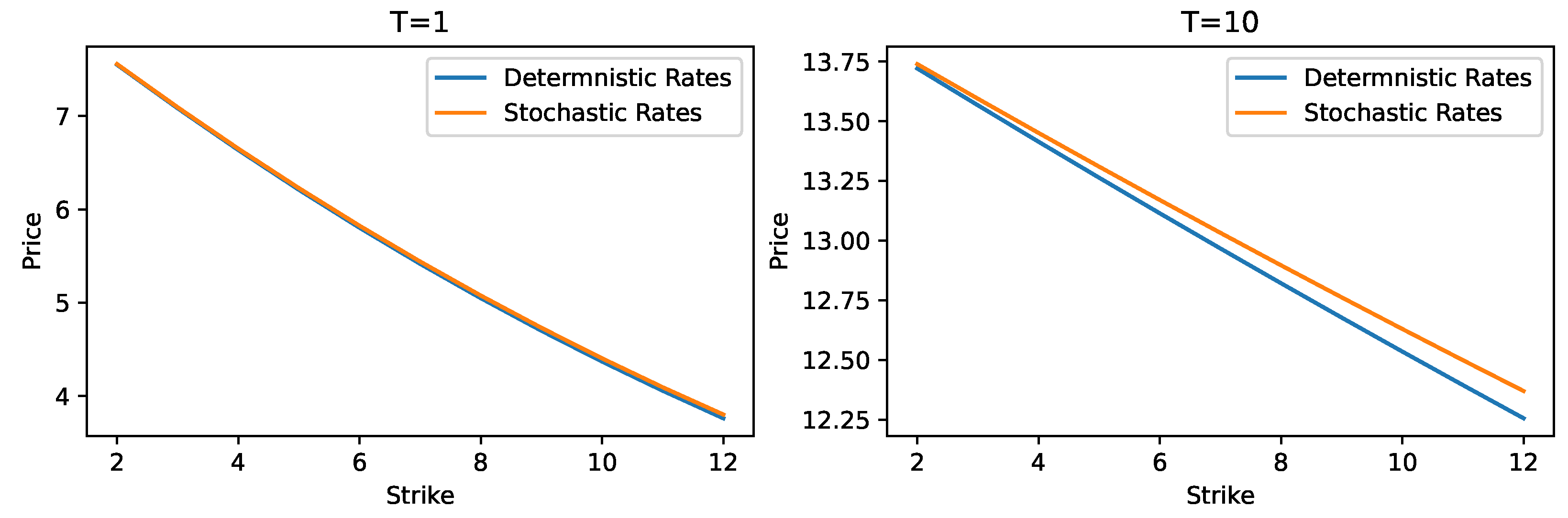
6.3. Impact of Stochastic Interest Rates

We consider the following two cases to test the impact of stochastic interest rates: Case 1 where interest rates and equity prices are positively correlated; and Case 2 where interest rates and equity prices are negatively correlated.

Figure 2 below shows the results for Case 1 using the same parameters as in Table 1 except for $\eta$, ${\rho }_{x_1,r}$, and ${\rho }_{x_2,r}$.

Similarly, Figure 3 below shows the results for Case 2.

For short-dated European spread call options, the impact of stochastic interest rates was insignificant. However, for long-dated European spread call options, the price difference between deterministic interest rates and stochastic interest rates widened for further out-the-money options. Moreover, when interest rates and stock prices were positively correlated, the spread option price under the stochastic interest rates was higher than under the deterministic interest rates. The opposite held when interest rates and stock prices were negatively correlated.

7. Conclusions

In this paper, we extended the Heston-Hull–White model of Grzelak and Oosterlee (2011) to two underlying assets and the FFT algorithm of Hurd and Zhou (2010) to account for stochastic interest rates.

Based on our implementation of the two-asset Heston–Hull–White model, we observed that the FFT algorithm was approximately 50 times faster than the Monte Carlo simulation. We also observed that the price of a long-dated European spread call option was sensitive to stochastic interest rates and equity-rate correlation. This difference became more significant for out-of-the-money options.

We hope that practitioners will find use in our extensions of the Heston–Hull–White model of Grzelak and Oosterlee (2011) and the FFT algorithm of Hurd and Zhou (2010), which will lead them to test the impact of stochastic interest rates on their spread option portfolios.

References

1. Alam, Md. Mahmudul, and Gazi Uddin. 2009. Relationship between Interest Rate and Stock Price: Empirical Evidence from Developed and Developing Countries. International Journal of Business and Management 4: 43–51. [Google Scholar] [CrossRef] [Green Version]
2. Alfeus, Mesias, and Erik Schlögl. 2018. On Numerical Methods for Spread Options. Research Paper Series 388; Sydney: Quantitative Finance Research Centre, University of Technology. [Google Scholar]
3. Carr, Peter, and Dilip Madan. 1999. Option valuation using the fast Fourier transform. Journal of Computational Finance 2: 61–73. [Google Scholar] [CrossRef] [Green Version]
4. Cox, John C., Jonathan E. Ingersoll Jr, and Stephen A. Ross. 1985. A Theory of the Term Structure of Interest Rates. Econometrica 53: 61–73. [Google Scholar] [CrossRef]
5. Dempster, Michael Alan Howarth, and SS George Hong. 2002. Spread option valuation and the fast Fourier transform. In Mathematical Finance-Bachelier Congress 2000. Berlin/Heidelberg: Springer, pp. 203–220. [Google Scholar]
6. Duffie, Darrell, Jun Pan, and Kenneth Singleton. 2000. Transform Analysis and Asset Pricing for Affine Jump-Diffusions. Econometrica 68: 1343–76. [Google Scholar] [CrossRef] [Green Version]
7. Grzelak, Lech Aleksander. 2011. Equity and Foreign Exchange Hybrid Models for Pricing Long-Maturity Financial Derivatives. Ph.D. thesis, Delft University of Technology, Delft, The Netherlands. [Google Scholar]
8. Grzelak, Lech A., and Cornelis W. Oosterlee. 2011. On the Heston Model with Stochastic Interest Rates. SIAM Journal on Financial Mathematics 2: 255–86. [Google Scholar] [CrossRef] [Green Version]
9. Heston, Steven L. 1993. A Closed-Form Solution for Options with Stochastic Volatility with Applications to Bond and Currency Options. The Review of Financial Studies 6: 327–43. [Google Scholar] [CrossRef] [Green Version]
10. Hull, John, and Alan White. 1990. Pricing Interest-Rate-Derivative Securities. The Review of Financial Studies 3: 573–92. [Google Scholar] [CrossRef] [Green Version]
11. Hurd, Thomas R., and Zhuowei Zhou. 2010. A Fourier transform method for spread option pricing. SIAM Journal on Financial Mathematics 1: 142–57. [Google Scholar] [CrossRef]
12. Kammeyer, Holger, and Joerg Kienitz. 2012. The Heston-Hull-White Model Part I: Finance and Analytics. Wilmott Magazine 2012: 46–53. [Google Scholar] [CrossRef]
13. Roberts, Jessica Ellen. 2018. Fourier Pricing of Two-Asset Options: A Comparison of Methods. Master’s thesis, University of Cape Town, Cape Town, South Africa. Available online: http://hdl.handle.net/11427/28126 (accessed on 25 February 2022).
Figure 1. Monte Carlo convergence using the parameters in Table 1.
Jrfm 15 00504 g001
Figure 2. Impact of stochastic interest rates with η = 0.05 , ρ x 1 , r = 0.75 , and ρ x 2 , r = 0.6 .
Jrfm 15 00504 g002
Figure 3. Impact of stochastic interest rates with η = 0.05 , ρ x 1 , r = 0.75 , and ρ x 2 , r = 0.6 .
Jrfm 15 00504 g003