Article

The Effects of the COVID-19 Crisis on Risk Factors and Option-Implied Expected Market Risk Premia: An International Perspective

1
Department of Financial Economics and Accounting, University of Alicante, San Vicente del Raspeig, 03690 Alicante, Spain
2
Department of Economics and Business, CEU Cardenal Herrera University, Reyes Católicos 19, 03204 Elche, Spain
*
Author to whom correspondence should be addressed.
J. Risk Financial Manag. 2022, 15(1), 13; https://doi.org/10.3390/jrfm15010013
Submission received: 2 December 2021 / Revised: 21 December 2021 / Accepted: 22 December 2021 / Published: 3 January 2022
(This article belongs to the Special Issue COVID-19’s Risk Management and Its Impact on the Economy)

Abstract

:
Institutional investors often have to decide which strategy to use across international business cycles. This is especially important during economic and financial crises. The exogenous nature of the outbreak of the dramatic COVID-19 crisis represents a unique opportunity to understand the performance of risk factors during severe economic times across international stock markets. Even more important is to analyze how these factors behave across very different economic crises, such as the COVID-19 pandemic and the Great Recession. Although, the overall results show that the momentum and quality factors are the winners, with the value factor as the loser, this research also reports different responses of factors across crises and countries. The size, value, and defensive factors tend to perform worse during the health crisis relative to the Great Recession, while the momentum factor shows a poor performance during the financial crisis, but a positive one during the outbreak of COVID-19. The quality factor is an extraordinary defensive factor in both crises. Similarly, this paper reports heterogeneous responses of option-implied expected market risk premia across alternative stock market indices, and between the Great Recession and the COVID-19 crisis.
JEL Classification:
G11; G12; G15

1. Introduction

Most existing investment industries follow a simple portfolio selection strategy based on a combination of the stock market portfolio and bonds. However, this combination tends to have a very high correlation with a 100% investment in the stock market. Given the extremely painful investment records of the market return during financial crises, especially during the Great Recession, the so-called factor investing is becoming popular and expanding rapidly among institutional investors. As Asness et al. (2015c) point out, institutional investors have turned their interest to strategies carrying alternative sources of return with relatively little correlation to the traditional market return. Factor investing consists of taking positions in systematic risk factors and thus being long and short in opposite characteristics. For example, a value investment style applies to long value firms (those with the highest book-to-market ratio) and to short growth firms (those with the lowest book-to-market ratio). This strategy replicates the return on the value factor of Fama and French (1993). A factor investment strategy is defined by Asness et al. (2015c) as the simultaneous long-short systematic and disciplined strategy that delivers long-term positive average returns across markets and asset classes, with overall low correlation with long-only portfolios.
The asset pricing literature has shown an enormous number of variables that supposedly explain the cross-sectional variation of average equity returns. Therefore, investors who want to follow a factor investment strategy are invaded by dozens of proposals claiming success by assuring positive and significant risk-adjusted returns or alphas. However, on the one hand, this proliferation of factors is certainly disturbing because theory shows that risk factors should be pervasive across assets and markets (Harvey et al. 2016; Clarke 2021; Jensen et al. 2021). On the other hand, these positive alphas are disguised into large portfolios that are exposed to the market. This implies that investors willing to pay fees to obtain alphas end up paying for market exposure or beta. For this reason, financial research conducting analyses of investment performance must be particularly careful in choosing risk factors. The selected factors should not only be economically motivated, but they should have also proven sound out-of-sample success across many asset classes and stock markets around the world.
Given the increasing popularity of factor investing, and the importance of diversifying strategies across international markets, especially during bad economic times, the objective of this paper is to analyze the performance of systematic risk factors across international stock markets during the COVID-19 crisis.
The previous discussion points towards a well-founded selection of risk factors in any research related with the performance of investment strategies. The factors analyzed in this paper are the classic Fama–French (1993) three factors, namely, the excess market return (MKT), and the size (SMB) and value-growth (HML) factors, together with the momentum (MOM) factor proposed by Carhart (1997), and two factors inspired by popular investing strategies based on quality and low risk: the quality minus junk (QMJ) factor of Asness et al. (2019), and the betting against beta (BAB) factor of Frazzini and Pedersen (2014), also known as the low-risk or defensive factor. The selection of these factors responds to three criteria. First, the selected factors must be sensitive to real activity. Rossi and Timmermann (2015) show that real activity, as a proxy for consumption and investment opportunities, plays a significant role in explaining the time-varying behavior of expected market risk premia. Given that expected excess returns are the product of the price of risk and the quantity of risk, and that uncertainty and risk aversion are embedded in the price of risk, the chosen factors must be exposed to shocks in both uncertainty and risk aversion as the key channel connecting the expected risk premia with the real economy. González-Sánchez et al. (2018, 2020) show that value, momentum, quality, and defensive factors present strong economic foundations given their relationship with uncertainty and risk aversion. Moreover, Maio and Philip (2018) show that economic activity plays a key role in explaining the anomalies associated with momentum. Second, the factors should generate time-varying expected risk premia. Zhang (2005) shows that value stocks are riskier because during bad times they are burdened with more unproductive capital and, when these firms want to disinvest, they face higher adjustment costs, and Kelly et al. (2021) show that momentum captures time-varying risk compensation. Asness et al. (2019) show that the quality factor is a powerful hedging strategy against bad times, and Frazzini and Pedersen (2014) argue that the defensive factor reflects funding liquidity. The size factor is also included given the relevance of this style if investors control by junk (Asness et al. 2018).1 Third, the selected factors must hold up across a multitude of asset classes, stock markets, and time periods. The papers by Asness et al. (2013); Israel and Maloney (2014); Asness et al. (2015c); Asness et al. (2015a, 2015b); Asness et al. (2018); Clarke (2021) discuss the risk factors that are proven to be pervasive styles across asset classes and markets. Moreover, these papers also identify those factors that successfully explain not only the unconditional, but also the conditional time-varying expected risk premia. The value, momentum, quality, and low risk factors, together with the carry factor (higher-yielding assets show higher returns than lower-yielding assets) that is especially popular in currency investing, are the more relevant examples satisfying these characteristics.
This paper conducts an extensive unconditional and conditional analysis of the behavior of these factors across international markets during the COVID-crisis period in comparison with, on the one hand, a stable pre-COVID period and, on the other hand, the Great Recession period. How different is the performance of the alternative risk factors across stock markets during the recent pandemic times? What factors and countries suffered the most from the effects of the recent exogeneous health shock? How different is their performance when comparing two extraordinary global crises that are very distinct in nature? The main contribution of this paper is to provide convincing answers to these questions. Given the international framework and, even more importantly, the focus on distinctly poor economic times, the analysis should provide a better understanding of the truly pervasive foundations of risk factors around the world.
In addition, both crises significantly increased risk aversion, which could have amplified the effects of global uncertainty and the associated sell-off in equities across international markets. It thus seems appropriate to study the behavior of risk factors when confronted with extreme increases in risk aversion and, therefore, in expected market risk premia. To understand potential differences in this sense, this paper also evaluates the performance of expected market risk premia, estimated from option prices with one-month and 12-month maturities on selected stock market indices around the world, comparing the COVID-crisis and the Great Recession periods.
Along these lines, Spatt (2020) has performed a comprehensive descriptive and theoretical comparison between the COVID-19 crisis and the Great Recession. Although, from an economic analysis perspective, the COVID-19 crisis differs fundamentally from the Great Recession due to the exogenous nature of the underlying shocks, there are similarities. Both crises highlight that the key risk supported by market participants is systematic risk, which lies on the core of asset pricing principles. In their analysis, Ramelli and Wagner (2020) focus on the role of firms’ exposure to international trade, and evaluate the stock price reaction to the COVID-19 crisis of the firms in the Russell 3000 index. They also show that the real effects from the pandemic are amplified through financial channels. It is therefore important to study the behavior of aggregate risk factors across both crises within an international context.
The remainder of the paper proceeds as follows. Section 2 describes the data. Section 3 reports and comments the descriptive statistics and risk-adjusted performance for the different factors and countries, comparing the COVID and pre-COVID subperiods. Section 4 analyzes the Great Recession and the COVID-19 crises in terms of the cumulative returns of risk factors and expected risk market premia. Section 5 provides a general discussion of the main findings of the research. Finally, Section 6 concludes the paper.

2. Data

This research employs daily international factor returns downloaded from AQR Capital Management’s database (www.aqr.com, accessed on 20 May 2020). This database contains factor returns at monthly and daily frequency for 24 countries: 16 from Europe, 4 from Asia, 2 from Oceania, and 2 from North America. In addition, it provides 5 aggregate equity portfolios, one of them being the world global index. However, the availability of the data differs between factors and countries. The sample used in this paper consists of 12 out of the 24 available countries plus the global market portfolio. The selection responds to the following reasons: (i) all geographical areas are represented in the sample, (ii) the selected countries are those with the most representative stock markets for each geographical area, and (iii) the selection produces the largest homogeneous sample period for all factors and countries. Under these criteria, the sample consists of daily returns from January 1997 to April 2020. The countries are Switzerland, Germany, Denmark, Spain, France, Great Britain, Italy, and Netherlands from Europe, Australia from Oceania, Japan and Hong Kong from Asia, and United States (USA) from North America.
The analysis is carried out for seven aggregate factors: the three Fama and French (1993) factors, the momentum factor due to Carhart (1997), the quality factor of Asness et al. (2019), the defensive factor of Frazzini and Pedersen (2014), and the version of the HML factor due to Asness and Frazzini (2013), known as the Devil-HML factor (HML D). This last factor is constructed using monthly price updates in the book-to-market ratio rather than the annual updating employed for the original Fama–French HML factor.
The SMB and HML factors represent long positions in small and value companies and simultaneous short positions in big and growth firms, respectively. The MOM factor takes a long position in winners and a short position in losers during the previous year. The BAB factor is the return differential between leveraged low-beta stocks and de-leveraged high-beta stocks. Frazzini and Pedersen (2014) show that leverage constraints are strong and significantly reflected in the return provided by this factor. They argue that the positive and highly significant risk-adjusted returns relative to traditional asset pricing models exhibited by portfolios sorted by the level of market beta are explained by shadow cost-of-borrowing constraints.2 Finally, a recent line of research identifies a quality stock as an asset for which investors would be willing to pay a high price, which means that these stocks are simultaneously safe (low beta), profitable (high return on equity), growing (high cash flow growth), and well managed (high dividend payout ratio). Asness et al. (2019) focus on a broad composite or umbrella series of three subgroups, namely, profitability, growth, and safety, to construct a risk factor using the Fama–French (1993) dollar-neutral weighting scheme. The QMJ factor buys high-quality stocks and shorts low-quality (junk) stocks.3
The analysis in Section 3 compares descriptive statistics and risk-adjusted returns for the different risk factors and countries between the COVID and the pre-COVID subperiods. The COVID subperiod is defined as the first quarter of 2020, coinciding with the first wave of the pandemic. The pre-COVID sample comprises the first quarter of each year between 1997 and 2019. The idea is to contrast the behavior of an exogenous crisis with a relatively long sample period controlling for the potential seasonality associated with the first months of the year.
Section 4 compares international stock markets during the Great Recession and the COVID-19 crisis. First, the comparison uses daily cumulative returns for the risk factors along the two subperiods. The Great Recession is defined using the National Bureau of Economic Research (NBER) recession months of the USA economy, from 1 October 2007 to 31 August 2009. To save space, and given the results reported in Section 3, in this case the exercise is performed using the global market and six representative international stock markets: Germany and Great Britain from Europe, Japan and Hong Kong from Asia, and Australia and the United States.
Second, the differential performance of international stock markets between the Great Recession and the COVID-19 crisis is also evaluated in terms of expected risk premia. Expected risk premia are estimated on a daily basis using option prices on stock indexes for two alternative maturities: one- and 12-months expiration horizons. Option data are from OptionMetrics’ IvyDB Global Indices database, which holds information on option prices on alternative international stock indexes. There is a total of 17 available indexes representing stock markets at both country and area levels. Since the sample of countries are not the same as those used in the analysis of risk factors, this study selects the most representative indexes of the different economic areas worldwide: the S&P500, the FTSE 100, the Euro Stoxx 50, and the Nikkei 225. To make the two periods comparable in terms of length, this analysis centers on the worst months within the Great Recession period.

3. The COVID-19 Crisis versus the Pre-COVID Period: Factor Returns

This section provides an international comparison of the risk factors’ performance between the problematic period defined by the first wave of the COVID pandemic, from 1 January 2020 to 31 March 2020, and a stable and long sample period pre-crisis that contains the first three months of each year between 1997 and 2019. The selection of the three first months is to control for potential seasonality effects that could make the two samples not comparable. First, in Section 3.1, the analysis provides descriptive statistics of factor returns. Then, alphas, estimated by the CAPM and the Fama–French models, are compared in Section 3.2.

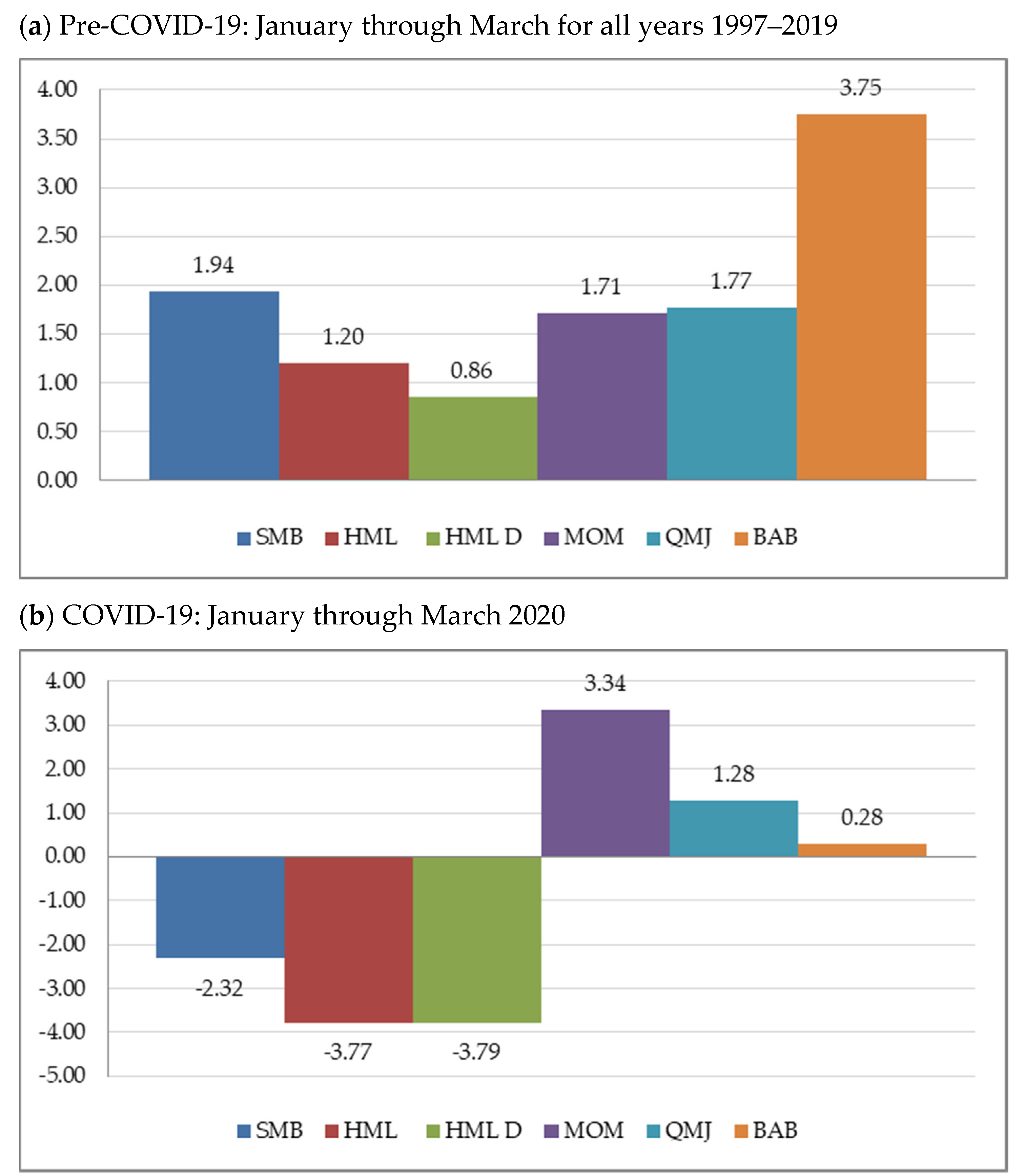
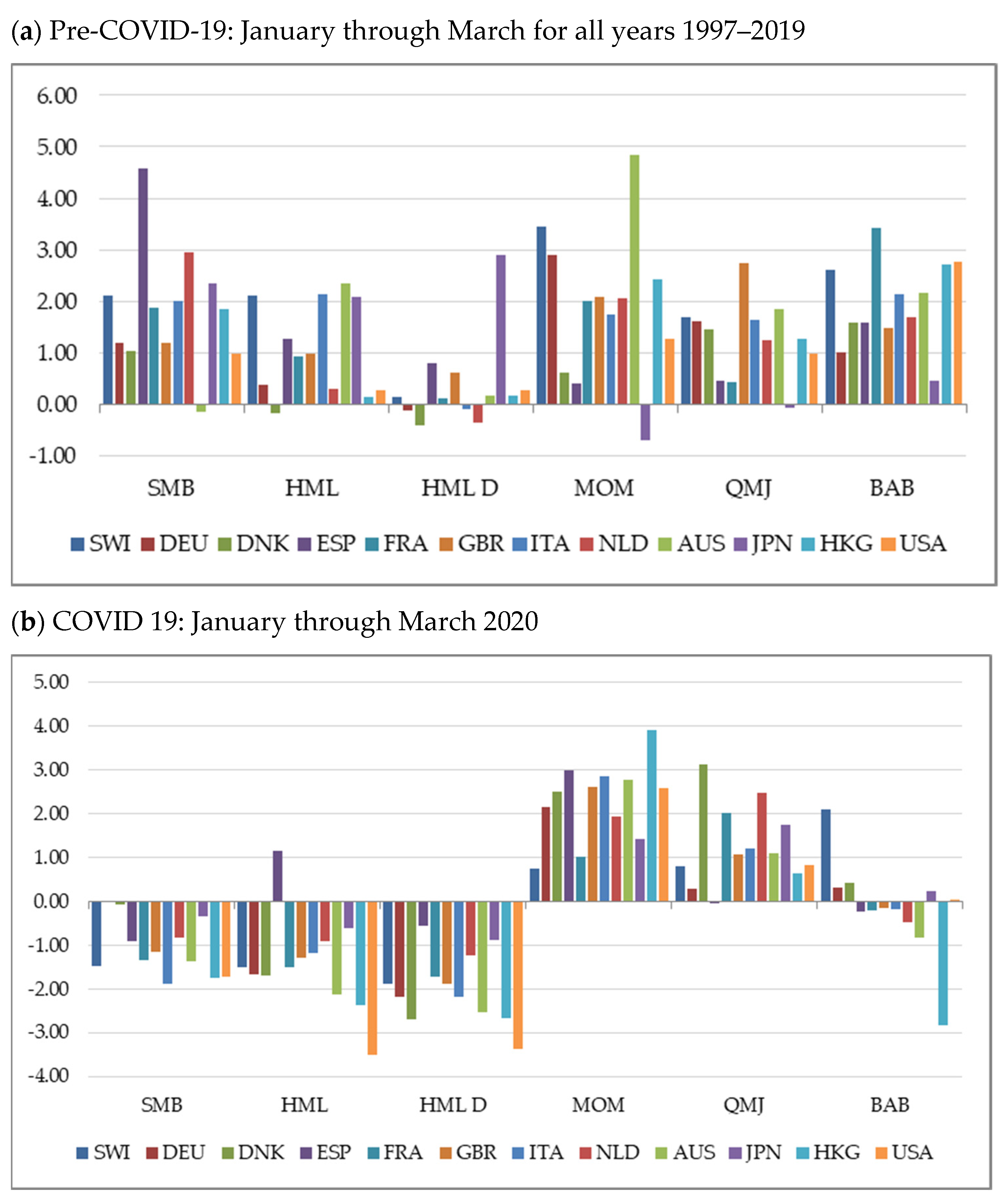
3.1. Mean Returns, Volatilities, and Sharpe Ratios

Panel A of Table 1 shows the average annualized market excess returns and the average annualized returns of the six additional risk factors for the 12 stock market indices and the global market portfolio during the first three months (January through March) of each year, from 1997 to 2019. Panel B reports the same statistics for the first three months of 2020, where the extraordinary outbreak of the COVID-19 crisis is captured. Similarly, Table 2 contains the results regarding annualized volatilities. Given that the patterns reported in average returns and volatilities are not necessarily homogeneous, the analysis avoids specific discussion about the results of these two tables, to concentrate the discussion on the Sharpe ratios across countries and factors. In any case, the information on means and volatilities contained in Table 1 and Table 2 provide the details for a better comprehension of the Sharpe ratios shown in Table 3. It is mentionable that market volatility is much higher during the COVID-19 crisis sub-sample for all stock exchanges, as expected given the rapid outbreak of the health crisis. On the other side, since factors reflect simultaneous long and short equity positions, the differences in volatility are not as large as for the market. The exception is the BAB factor reflecting the uncertainty embedded during COVID-19 regarding funding liquidity.
Panels A and B of Table 3 display the Sharpe ratios for both sample subperiods. During the 1997–2019 period, the United States, due to its low volatility, and especially Denmark, due to its high average return, are the two countries with the highest market Sharpe ratios. It is interesting to point out that Denmark is also the stock market with the least negative Sharpe ratio during the health crisis. On the negative side, Japan, Hong Kong, Great Britain, and Spain present the worst results during the first quarter of the 1997–2019 period, with market Sharpe ratios all lower or equal to 20% compared to the 35.3% of the global index. Great Britain also shows the worst performance during the COVID-19 crisis, while France, Japan, Germany, Spain, and Australia present relatively worse performance than the other countries. Interestingly, Italy does not display extreme bad performance in terms of the market Sharpe ratio during the health crisis.4
Regarding the risk factors, in the pre-COVID subperiod, the MOM and BAB investment styles clearly outperformed the rest of the factors. In terms of the MOM Sharpe ratio, Australia, Great Britain, and Hong Kong warrant mention, and in terms of the BAB Sharpe ratio, the United States and Hong Kong dominate. Interestingly, Germany, a market with positive average skewness during the sample period, has the lowest BAB Sharpe ratio, while the USA market and the global portfolio have negative skewness values of −0.17 and −0.31, respectively. These results are consistent with the skewness explanation of the BAB factor as suggested by Schneider et al. (2020). The value factors generally present low Sharpe ratios, reflecting the relatively bad performance of value investing during the last twenty years. Finally, given the well-known hedging performance of the QMJ factor, it is not surprising that its Sharpe ratio during the pre-COVID period is relatively low, resembling the behavior of the value factors during those years and quarters.
During the first quarter of 2020, the market returns, SMB, and the two HML factors, present negative Sharpe ratios for almost all the countries, highlighting the bad performance of the two value factors. This new evidence confirms that systematic investing in value is highly risky, due to its poor performance during extremely distressing times. However, as emphasized by Israel et al. (2021), the suggestion that value investing is dead seems to be premature. In contrast, the QMJ and MOM, and BAB factors show positive results for some stock markets. Among the 12 countries, Denmark, the Netherlands, and Japan have the highest average QMJ returns, and only the United States has small, negative average QMJ return. The MOM factor has a positive and impressive global Sharpe ratio during the COVID-19 crisis. Hong Kong, and Spain are the best momentum performers during the crisis, but Great Britain, Italy, and the United States are also good momentum performers. Since the BAB factor reflects funding liquidity and skewness, its performance is globally negative during the health crisis. In contrast, this factor’s performance in Switzerland is impressive suggesting the country’s extreme reputation for safety. Germany and Denmark also show strong BAB performance, which is consistent with the idea of financial reputation.
To summarize, in the full first-quarter sample period from 1997 to 2019, which can be identified as the normal-time, the global BAB and MOM risk factors are the star performers. During the worst months of the pandemic crisis, the QMJ risk factor and, once again, the MOM factor have not only positive average returns, but also extraordinary Sharpe ratios relative to the overall market performance. On the negative side, the value factors present the worst performance in both normal and bad economic times.

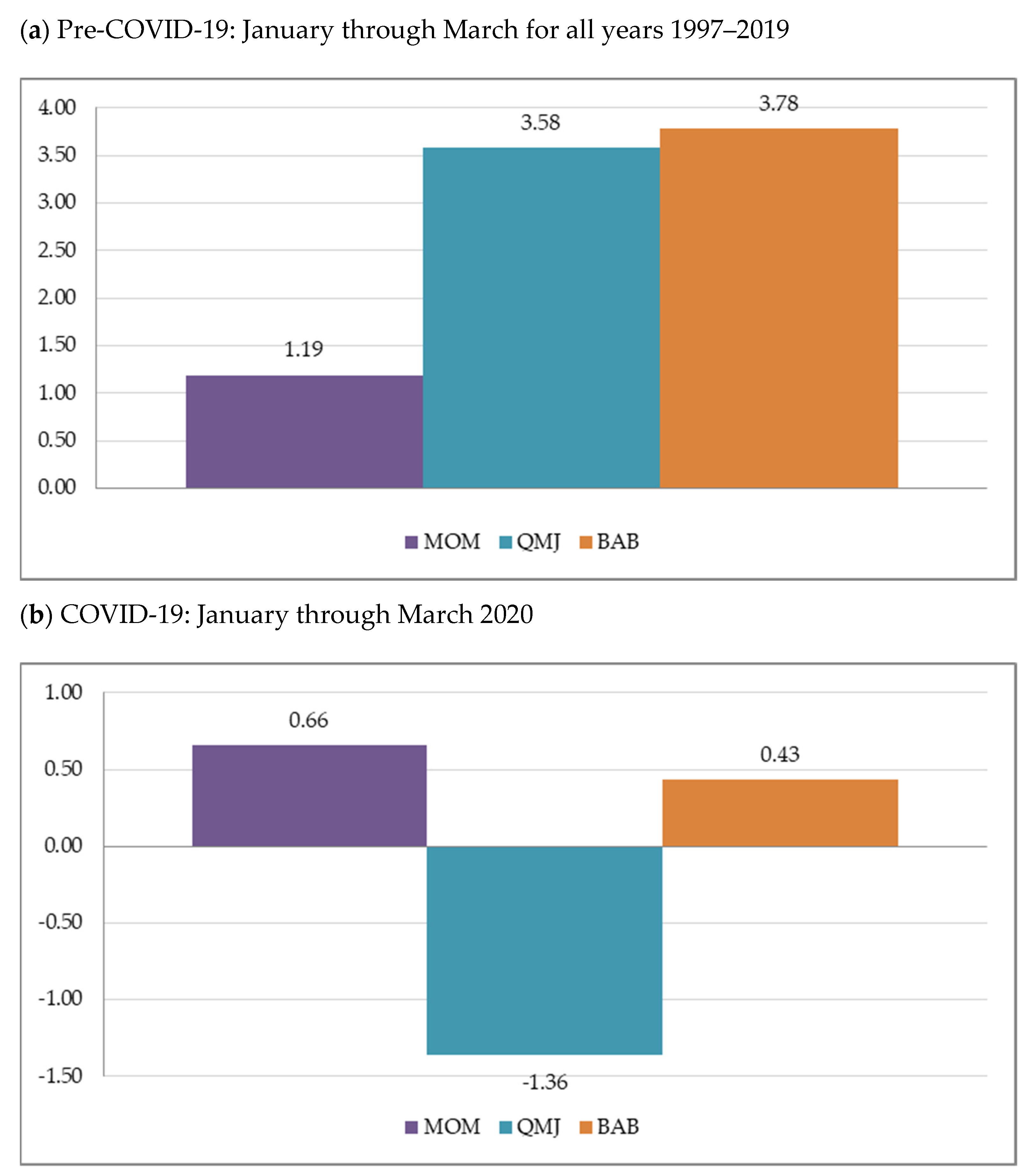
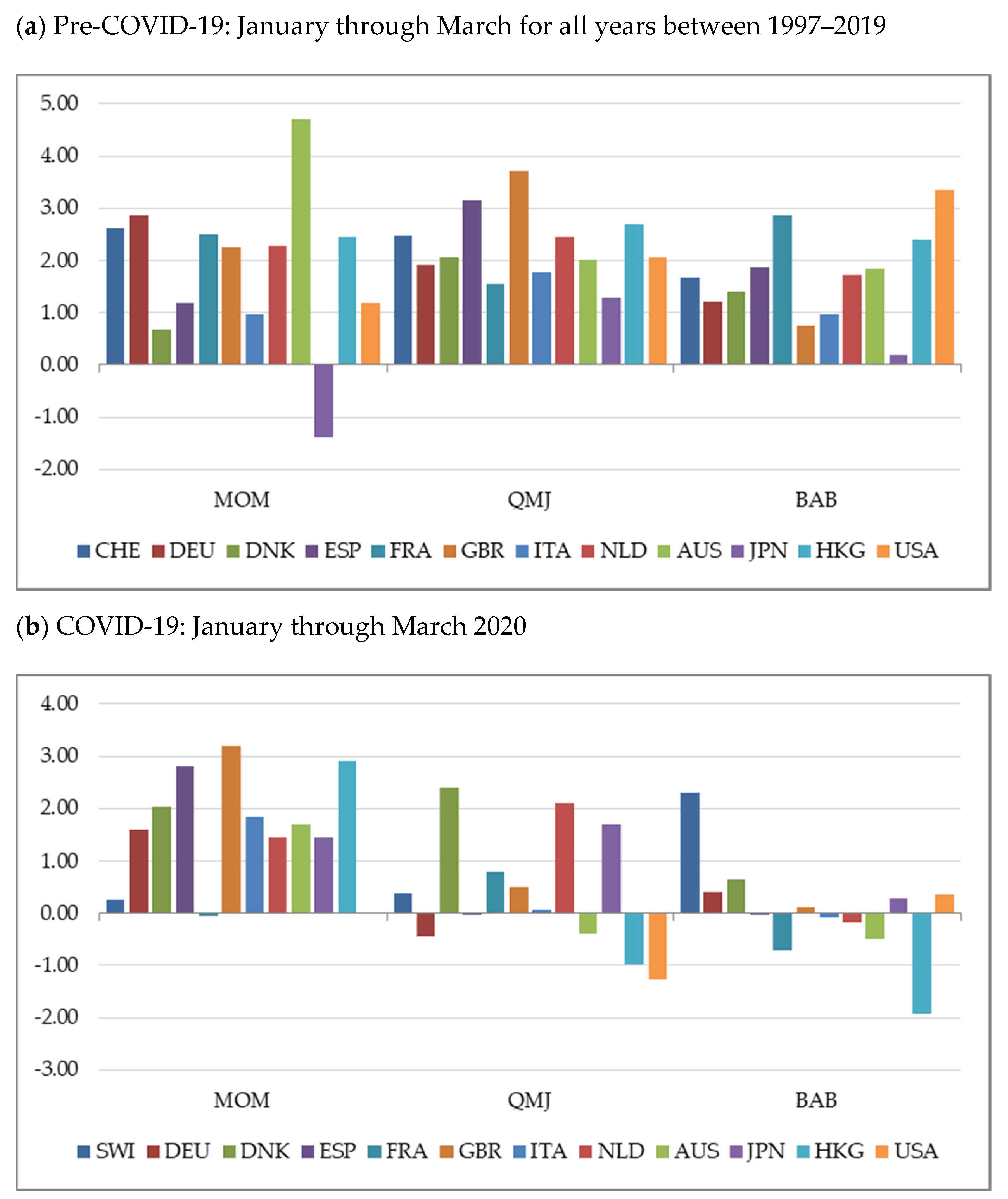
3.2. Risk-Adjusted Returns

This section provides estimation results of the CAPM alphas for each risk factor and country using the following ordinary least squares (OLS) regression:
F j t k = α j k + β j k M K T j t + ε j t k
where F j t k is the risk factor k in country j, from the set of six factors different from the market factor, M K T j t is the excess market return in country j, α j k is the market risk-adjusted performance of factor k in country j, and β j k is the market beta of risk factor k in country j. The research employs monthly data for the long sample period spanning the first quarters for each of the years from 1997 to 2019; on other hand, for the COVID period, the regression is run with daily data that comprises the three months of the first quarter of 2020. The results are reported in Panels A and B of Table 4, respectively. The (average) alphas reported in Panel A of Table 4 should be taken as a benchmark.
The overall results for the pre-COVID subperiod point out the heterogeneity of the performance across countries and risk factors. For the global index, only the BAB factor presents a positive and statistically significant alpha with an impressive value as high as 14.7% on annual basis. The SMB, MOM, and QMJ risk factors show positive alphas with t-statistics of 1.94, 1.71, and 1.77, respectively. Consistently with the results of Table 3, the value factors generate alphas with lower t-statistics, especially for the HML devil. Once again, relative to the market’s behavior, HML exhibits disappointing performance during the first quarters of the last 23 years. The t-statistics of the CAPM alphas for the global case are displayed in Figure 1a.
These results are not entirely consistent across countries. The SMB factor has positive and significant CAPM alphas for five countries with outstanding performance of 22.1% on an annual basis for Spain, and a strong performance of 12.8% on an annual basis for the Netherlands. The results for the value factors across stock markets are relatively poor. The HML factor with annual updating shows significant alphas in four countries. Things are worse for the devil version, however. The only country for which both value factors have positive and statistically significant alphas is Japan. Indeed, the CAPM value alphas for Japan are 15.8% and 7.1% for the devil and Fama–French versions, respectively. The MOM risk factor presents much better risk-adjusted performance across markets than the HML factor. Seven countries show positive and significant alphas. The range on an annual basis, goes from 26.7% for Australia, estimated with very high precision, to 12.1% for France, with a t-statistic of just 2.01. Germany, Switzerland, and Hong Kong also exhibit strong positive momentum performance. The QMJ alpha is quite stable across countries, but it is estimated with little precision for all the markets except for Great Britain’s. The BAB factor presents very good performance, not only globally, but also across countries. Six of them have positive and statistically significant alphas with no alphas on the negative side. Hong Kong, France, the United States, and Italy have significant alphas, higher than 15% on an annual basis.
Figure 2a shows the t-statistics of CAPM alphas for each country and factor estimated in the pre-COVID sample period. The figure illustrates the relatively good performance of the MOM and BAB factors and the overall worse performance of the HML factors across countries. Japan is a positive outlier in terms of the HML factors, and a negative outlier for the MOM factor. Also, it is the country with the lowest t-stat for the BAB factor. Therefore, despite the relevant heterogeneity of the performance of risk factors across countries, the results show a consistent overall picture when comparing Figure 1a and Figure 2a.
Panel B of Table 4 shows the CAPM alphas across countries and factors during the COVID-19 subperiod. For the global market, there is noticeable differences in the performance of two groups of risk factors. On the one hand, SMB and both HML factors present bad performance with highly negative and significant alphas. On the other hand, the MOM, QMJ, and BAB factors have positive alphas, although only the MOM factor alpha is significant. The performance of the MOM factor over and above the behavior of the market during the critical first quarter of 2020 is striking. The t-statistics for the CAPM alphas and the global index across factors are displayed in Figure 1b.
During the COVID-19 crisis, the results of the individual countries are consistent with global performance. For all the countries, the SMB and HML factors show negative alphas, with particularly negative and significant results for the two HML factors in the Australia, Hong Kong, and USA markets. On the opposite side is the MOM factor with positive alphas for all 12 countries, with significance for eight of them. The consistency of the MOM factor across capital markets during the first wave of the pandemic is a very important result for factor investing. Even more surprising is that Spain is the country with the highest significant positive alpha despite being extremely affected by COVID-19. The results of the QMJ and BAB factors are more heterogeneous with only three stock markets showing a positive and significant alpha: Denmark, France, and the Netherlands. Denmark is again a relevant example, showing positive and significant alphas for both the MOM and QMJ factors. The BAB factor shows less consistency across markets relative to the previous two factors. It is positive and significant only for Switzerland, but negative and significant for Hong Kong. The heterogeneous response across countries and factors could be associated with the evidence reported by Bretscher et al. (2020), who show that firms with labor-intensive industries and firms located in countries with a large mobility decline have exhibited worse stock market performance during the COVID-19 crisis. Figure 2b summarizes this discussion, showing the t-statistics for the individual countries and factors.
Table 5 reports the risk-adjusted performance across countries for the MOM, QMJ, and BAB risk factors using the Fama–French three-factor model. The analysis shows the annualized alpha values obtained from the following OLS regression:
F j t k = α j k + β j m k M K T j t + β j s m b k S M B j t + β j h m l k H M L j t + ε j t k ,
where F j t k is either MOM, QMJ, or BAB in country j. The HML factor used in the regressions is the HML devil.
In the pre-COVID-19 subperiod, the Fama–French alphas for the MOM factor are very similar to the CAPM alphas, confirming its significant performance in the same countries as before. Although the BAB alphas are positive for all the countries, they are now statistically significant only for France, Hong Kong, and the United States. In any case, the performance of the BAB factor continues to be strong (12.6% on an annual basis) globally. The QMJ factor once again shows a positive and significant result for the global index, although with a much more moderate global alpha of 6.7% relative to the BAB factor. The QMJ portfolio is now shown to be significant in eight countries. Figure 3a and Figure 4a illustrate these findings.
During the COVID-19 health crisis, none of the three factors presents significant alphas for the global index. Generally, and across countries, the Fama–French alphas are lower than the CAPM alphas. However, the MOM factor continues to show good performance in Denmark, Great Britain, Hong Kong, and especially Spain. These results are displayed in Figure 3b and Figure 4b.
In conclusion, the momentum investment strategy has a better risk-adjusted performance record relative to the other factors during the COVID-19 health crisis. For the global portfolio, it has a high and statistically significant CAPM alpha. When the MOM risk-adjusted return is computed from the Fama–French model, it is also positive, although not statistically different from zero. Contrary to the other factors, the MOM alphas are consistent across countries. They are positive for all countries and for both the CAPM and the Fama–French models.5 Moreover, during the COVID period in which all stock market returns show high losses, MOM alphas are significantly different from zero in eight (four) countries for the CAPM (Fama–French) model.

4. The Great Recession and the COVID-19 Crises: Cumulative Factor Returns and Expected Risk Premia

This section includes two alternative analyses aimed at comparing stock markets around the world and between two extraordinarily adverse crises: the Great Recession and the COVID-19 pandemic. The first part evaluates the behavior of the cumulative returns of risk factors, while the second analysis addresses option-implied expected market risk premia and their associated term structure.

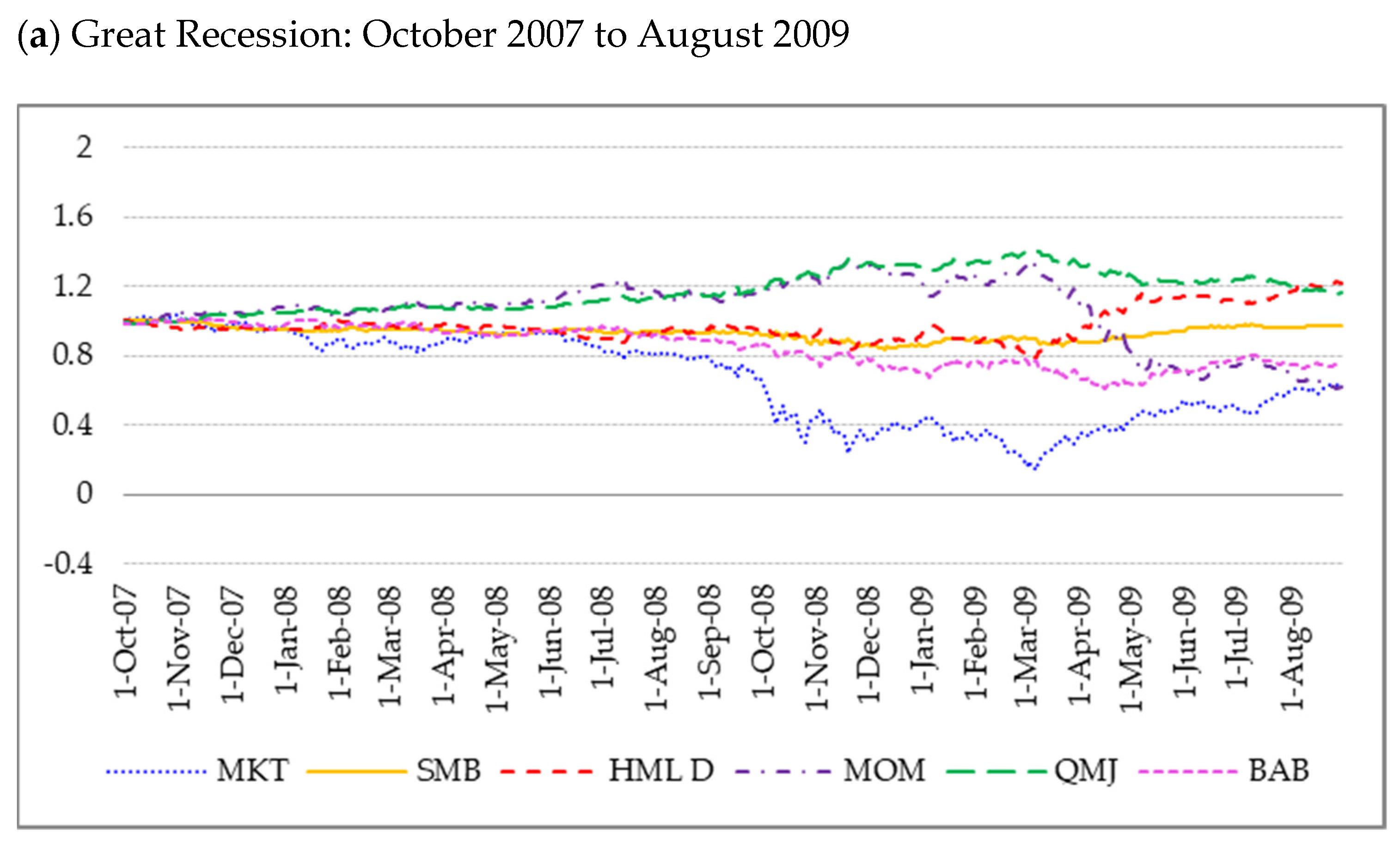
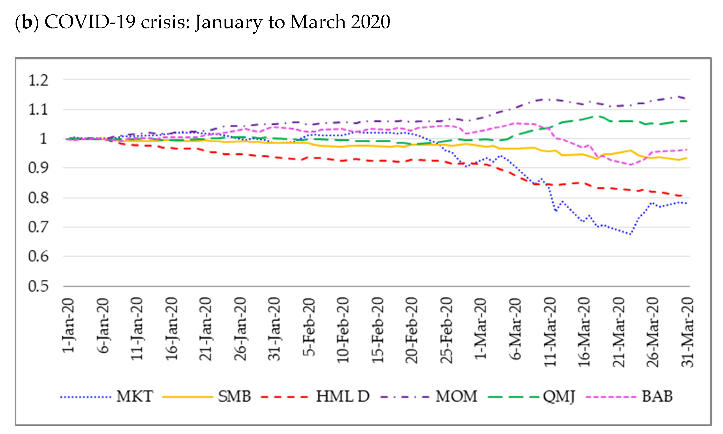
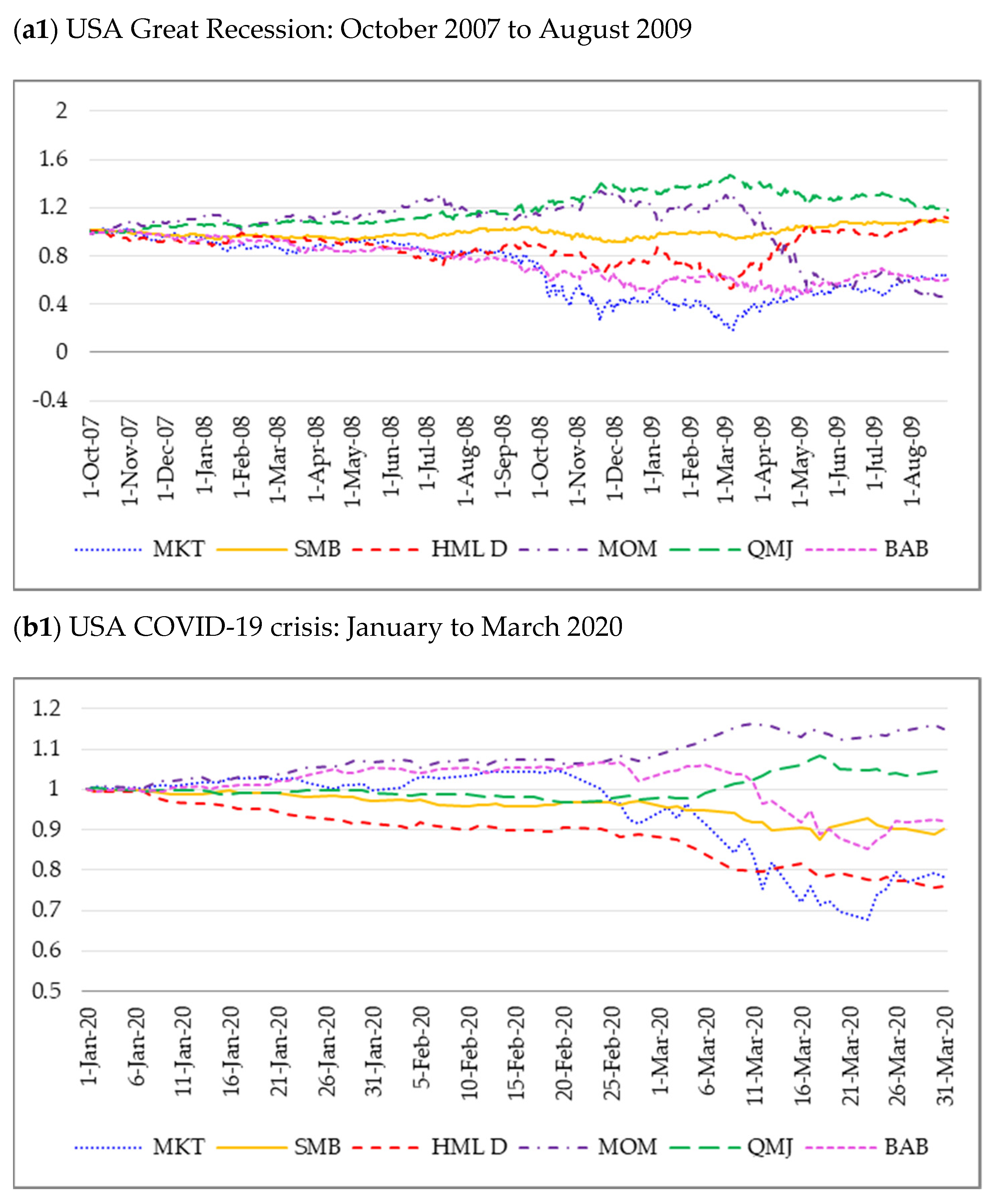
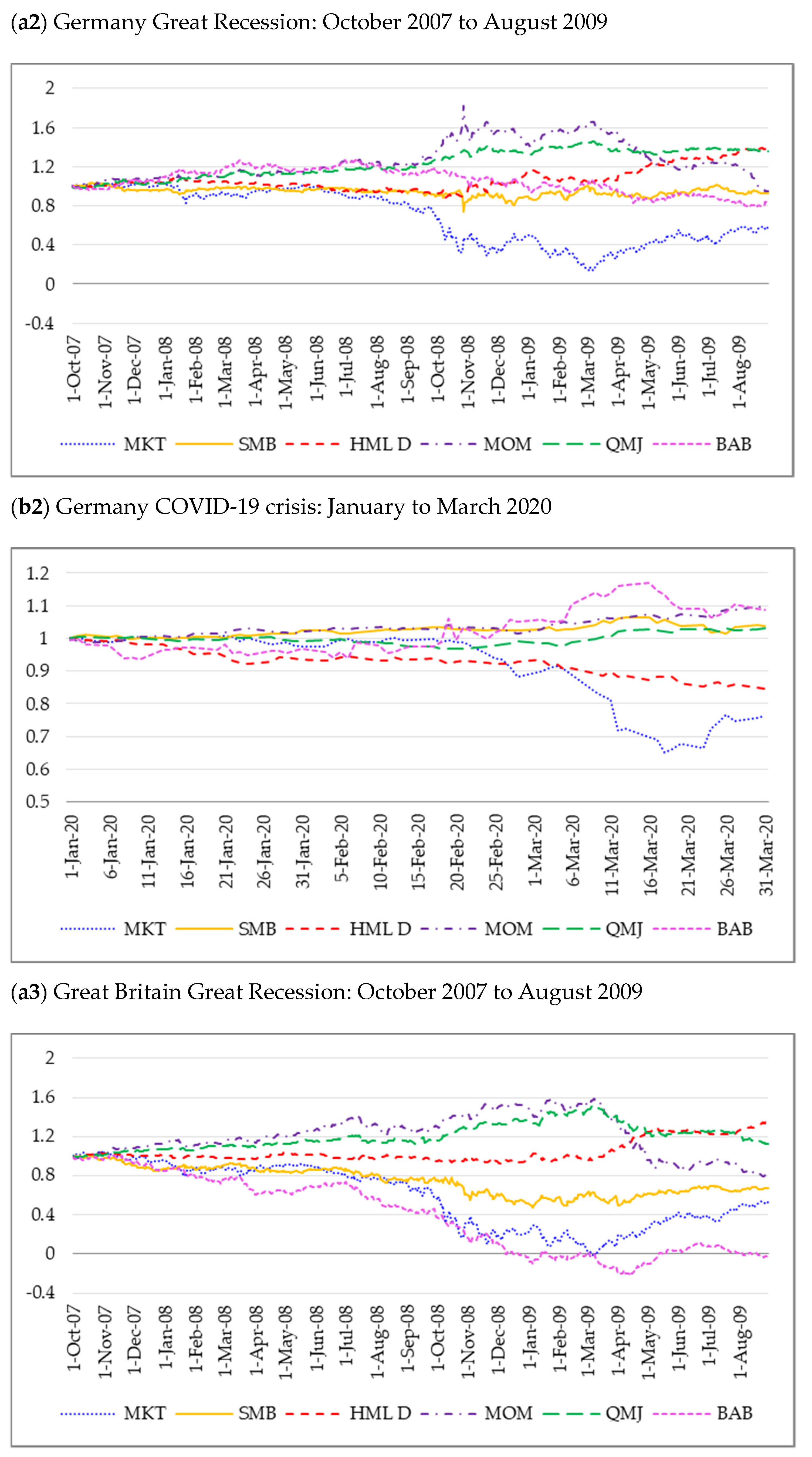
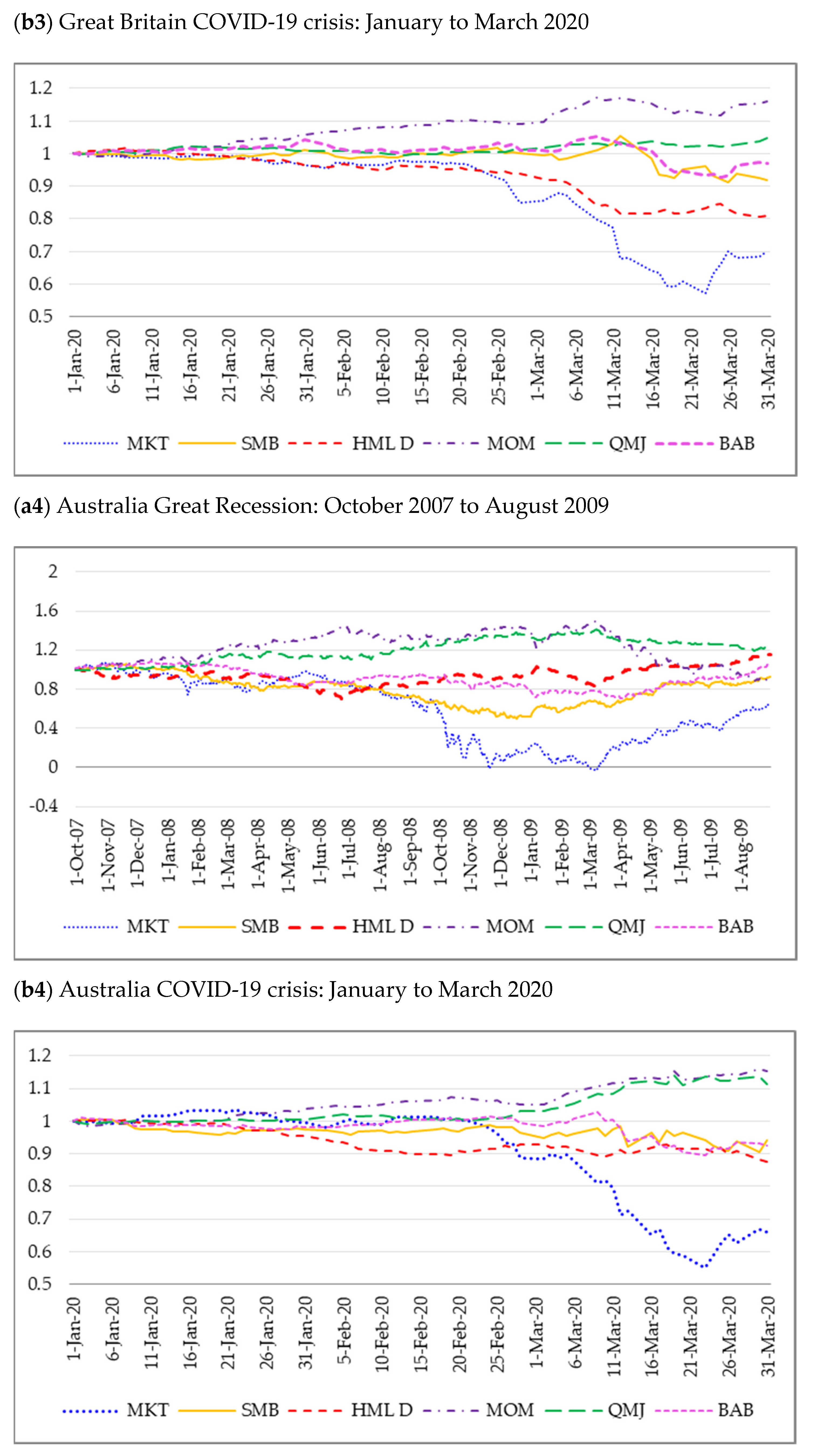
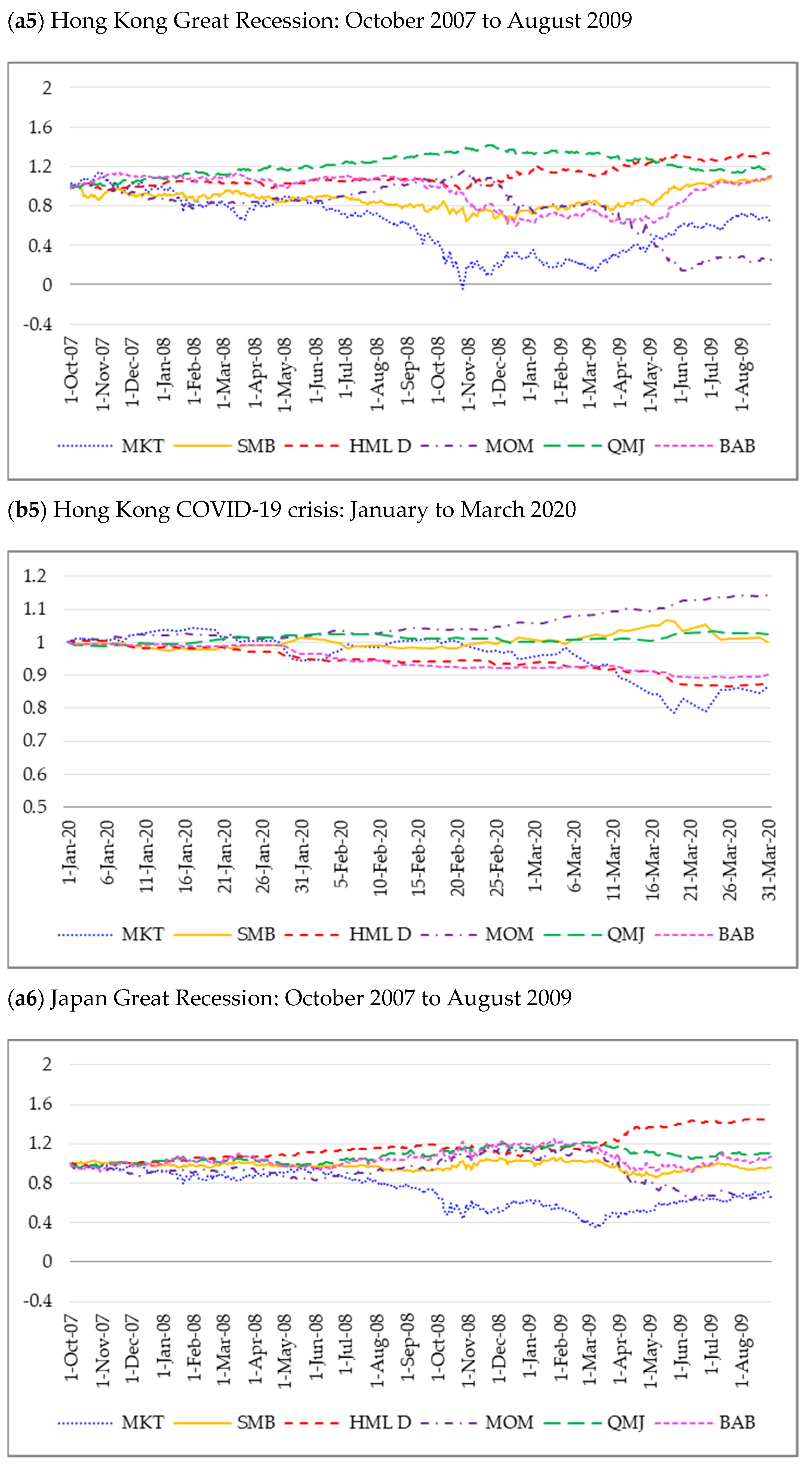
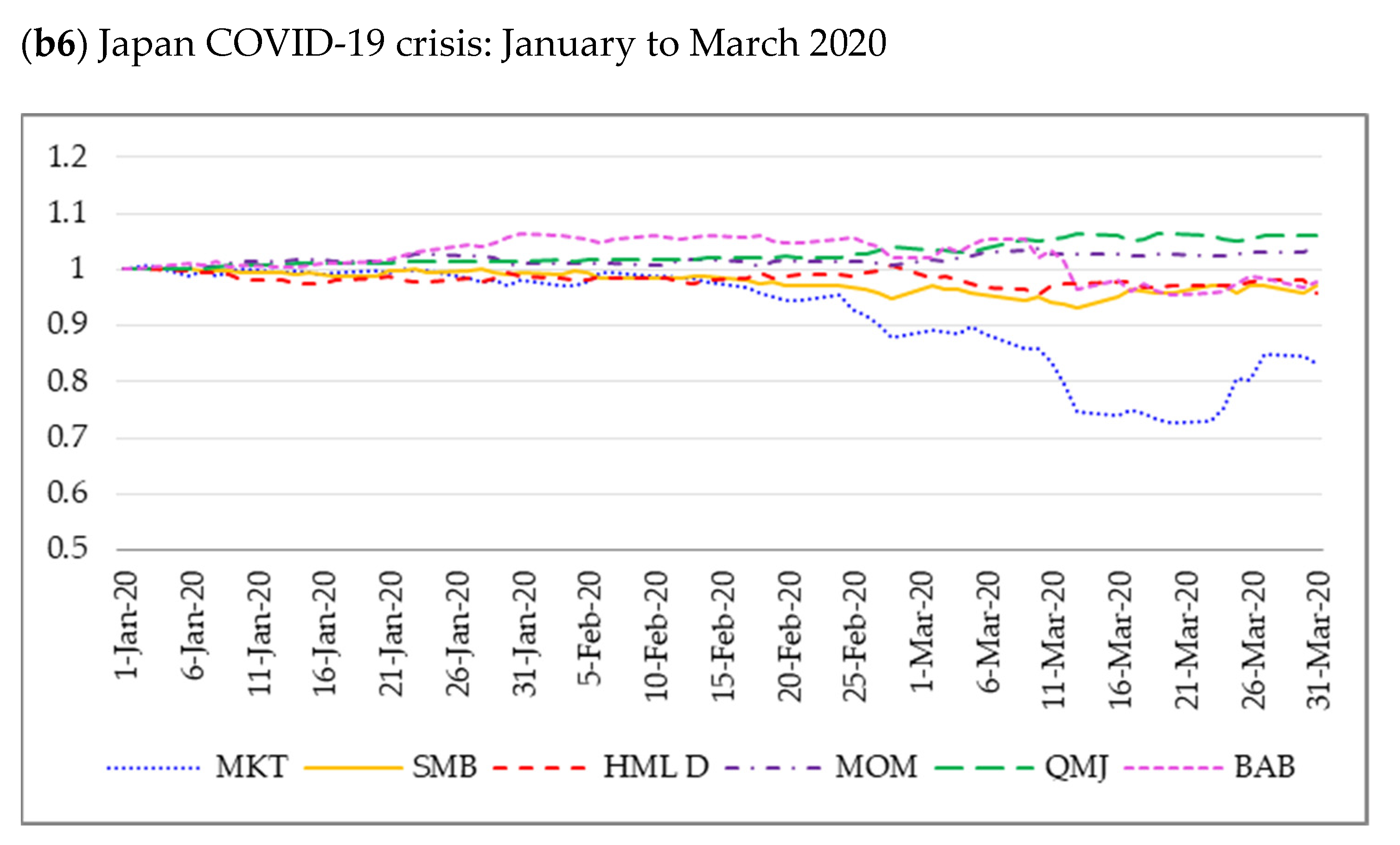
4.1. Cumulative Factor Returns

This sub-section presents a direct comparison between the behavior of the excess market returns and other six risk factors during the Great Recession and the COVID-19 crisis. The Great Recession is defined using the NBER recession months of the USA economy, from 1 October 2007 to 31 August 2009. The COVID period includes the first quarter of 2020. Using daily data, cumulative returns are computed for investing one dollar on 1 October 2007 and 2 January 2020, for the Great Recession and the COVID subperiods, respectively, for all seven risk factors. To save space, and given the evidence in the previous section, results refer to the global market and six representative international stock markets around the world: Germany and Great Britain from Europe, Japan and Hong Kong from Asia, Australia, and the United States.6
Table 6 displays the annualized minimum cumulative return in percentage terms, defined as the difference between the worst cumulative return during each subperiod and the return at the beginning of the corresponding subperiod. Panel A refers to the Great Recession and Panel B to the COVID-19 subperiod. The results shed light on how the risk factors react to the different natures of the two crises compared in the analysis. In both panels, the cumulative excess market return is negative in all countries and on the global portfolio. But the negative results are much more dramatic during the pandemic. This result is in line with the evidence provided by Baker et al. (2020) who show that, for the USA market, no previous infectious disease has ever affected the stock markets as much as COVID-19. Their evidence suggests that government restrictions largely explain this impact, especially in a service-oriented economy. Regarding the market performance across countries, particularly negative cumulative returns are shown for Great Britain and Australia. It turns out that these two markets also experienced the worst cumulative returns during the Great Recession.
This pattern between both subperiods is also found for the SMB, HMLs, and BAB risk factors. The cumulative performance of these factors is clearly more negative during the COVID-19 than during the Great Recession for both the global index and most countries. The impressive exception is the BAB in Germany during the first quarter of 2020. If the BAB factor reflects funding liquidity, the result suggests that investors discounted the extraordinary capacity of the German economy to provide direct financial resources to German companies. The cumulative behavior of the MOM factor is once again striking. Overall, the MOM factor presents the worst performance among the six factors analyzed during the Great Recession. However, the cumulative performance of the MOM factor during the COVID-19 subperiod is amazing. The momentum strategy experiences positive results in all the countries, especially in the cases of the Great Britain, Australian, Hong Kong, and USA stock markets. This evidence is consistent with the average results reported in previous sections. Moreover, given its hedging nature, as shown by Asness et al. (2019), the cumulative performance of the QMJ factor in both crises is positive both globally and across markets. Overall, the QMJ factor performs better in the COVID-19 pandemic than in the Great Recession, with especially good relative performance for Australia and Japan.
Figure 5 and Figure 6 show the time series evolution of cumulative returns along each subperiod for the global market and the six selected countries, respectively. Starting with the global index in Figure 5, the different effect of the two crises in the value and momentum factors is mentionable. During the Great Recession, the HML D factor shows a stable cumulative return that even starts increasing from March 2009 while, except for the market, it is the worst performer during the COVID crisis. On the contrary, the MOM factor shows an increasing trend during late 2007 and 2008 but experiences a big fall in March 2009. However, the MOM strategy supports very satisfactorily the COVID adverse shock, showing increasing cumulative returns during the first quarter of 2020. The QMJ factor shows consistent good behavior during the two crises.
Regarding the countries in Figure 6, the best performers during the Great Recession are the QMJ factor in general, the value factor for Great Britain, and the two Asian markets. The worst factor for this sub-period is MOM for most countries, and the BAB factor in the USA and Great Britain. In contrast, during the COVID sub-period, the best performers are the QMJ strategy and, especially, the MOM factor. Finally, except for the market, the HML D factor is the worst performer across the six risk factors.

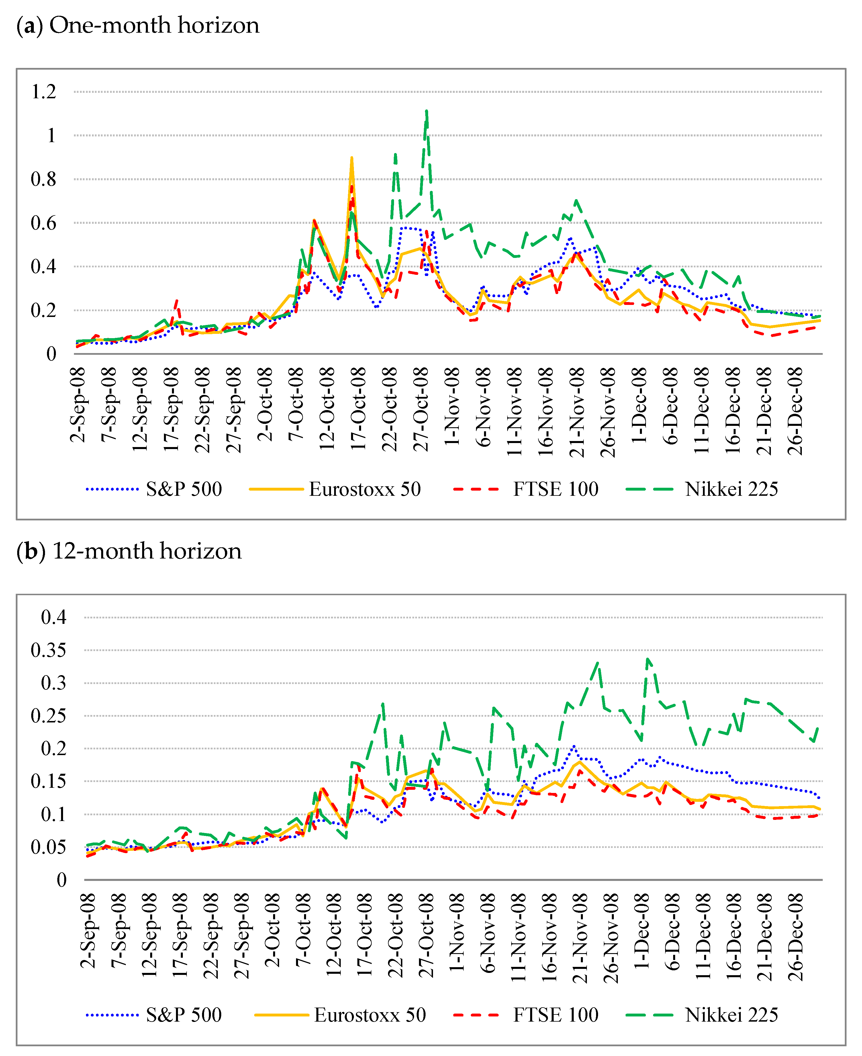
4.2. Expected Market Risk Premia

Until now, the analysis has focused on the average or cumulative past returns of the risk factors across markets. In this section, the evaluation moves toward a forward-looking framework by studying the behavior of the expected market risk premia. Hence, instead of analyzing the impact on stock returns, the focus is now investors’ expectations during the two largest global crises since the beginning of the 21st century.
To estimate expected equity risk premia, this research employs the information content of options prices. Jackwerth (2020), using options on the S&P 500 index, shows that risk-neutral distributions are more informative about the COVID-19 pandemic and the collapse of market expectations than the stock market index values.7 Ampudia et al. (2020) estimate a tail risk aversion indicator for the Euro Stoxx 50 constructed by comparing the left tails of the risk-neutral and physical distributions. Their evidence, consistent with the results provided by Jackwerth (2020), show that tail risk aversion increased from the second half of February 2020 to the second half of March 2020, as monetary and fiscal policies were introduced in North America and Europe.
Therefore, on the one hand, this section aims to analyze the behavior of expected equity risk premia in different geographical areas during the COVID-19 crisis and, on the other hand, to compare the level and the time-varying behavior of the expected risk premia between the two most important recent crises: The Great Recession and the pandemic crisis.

4.2.1. The Estimation Procedure of Expected Market Risk Premia

This paper uses the option-based approach developed by Martin (2017) rather than the more common approach based on dividend strips. As pointed out by Cochrane (2011), most of the variation in prices is due to changes in expected returns. Therefore, by using expected market returns, this study learns about changes in discount rates driven by risk aversion and/or uncertainty. Moreover, Gormsen and Koijen (2020) employ data from the dividend futures market to estimate growth expectations by maturity and find that the information of dividends is insufficient to explain the big drop in the stock market.8
Using the fundamental asset pricing equation, Martin (2017) shows that the expected market risk premium can be written as
E t P ( R m T ) R f t = 1 R f t V a r t Q ( R m T ) C o v t P ( M T R m T , R m T ) ,
where R m T is the gross market return between t and T, M T is the stochastic discount factor at time T, R f t is the gross risk-free rate from t to T available at time t, E t P ( ) and C o v t P ( ) are respectively the expectation operator and the conditional covariance under the physical probability at time t, and V a r t Q ( ) is the risk-neutral conditional variance at time t.
Martin (2017) points out that, if the relative risk aversion and the elasticity of intertemporal substitution are greater than one under recursive preferences, the following negative correlation condition holds:
C o v t P ( M T R m T , R m T ) 0 .
Under this condition, the risk-neutral variance normalized by the risk-free rate constitutes a lower bound for the expected market risk premium:
E t P ( R m T ) R f t 1 R f t V a r t Q ( R m T )
Thus, the estimation of the lower bound of the expected market risk premia basically consists of estimating the risk-neutral variance of market returns using option prices. Following Martin (2017), the following equivalence holds:
1 R f t V a r t Q ( R m T ) = 1 S t 2 [ 2 0 c a l l t , T ( K ) d K F t , T 2 R f t ] ,
where S t is the price of the underlying asset at time t, F t , T is the futre price of the underlying at time t with maturity at T, and callt,T is the price at time t of the option to buy the underlying at expiration T with strike price K. Martin prevents use of deep-in-the-money calls since they are illiquid and proposes their substitution with out-of-the-money options to sell (put) by using the put-call parity. Then, Equation (6) transforms into:
1 R f t V a r t Q ( R m T ) = 2 S t 2 [ 0 F t , T p u t t , T ( K ) d K + F t , T c a l l t , T ( K ) d K ] .
This study estimates the lower bound using Equation (6). However, instead of using call prices, only data on put prices are employed. Then, the implied volatility surfaces of put options are used to price the corresponding call options, instead of using the transformation given by the put-call parity. The estimation follows the procedure of Rubio et al. (2021).
Daily option data are from OptionMetrics’ IvyDB Global Indices database, which holds information on the options on the main international stock indexes for different maturities. This study selects the following underlying indexes as representative of the stock markets of the different economic areas worldwide: the S&P500, the FTSE 100, the Euro Stoxx 50, and the Nikkei 225.
It is widely accepted that the expected market risk premium is not only time-varying and counter-cyclical, but also different for alternative horizons. A very important finding in this respect is that the slope of the equity term structure changes over the business cycle. The slope tends to be significantly more negative during recessions.9 In fact, the term structure of expected equity returns plays a fundamental role in many financial decisions. The research employs two option maturities, one- month and 12-months, not only to obtain expectations of the risk premia for two different future horizons, but also to compute and analyze the slope of the term structure of the expected market risk premia during the two crises periods.
In this case, the COVID-19 sub-period is defined from January to April 2020. Different from the previous sections, this analysis includes April 2020 because during the second half of this month the number of contagions started declining from the peak observed in March. This inflection point is an important feature for understanding the time pattern of expected market returns. On the other hand, since now the analysis looks at expectations rather than past returns, it is important to employ the same duration for both crises to make the results comparable each other. Therefore, the sub-period representing the Great Recession is a four-month period that includes the three months with the worst market returns for all the selected indexes (October–December 2008) and September 2008 to capture the possible anticipation from investors’ expectations.

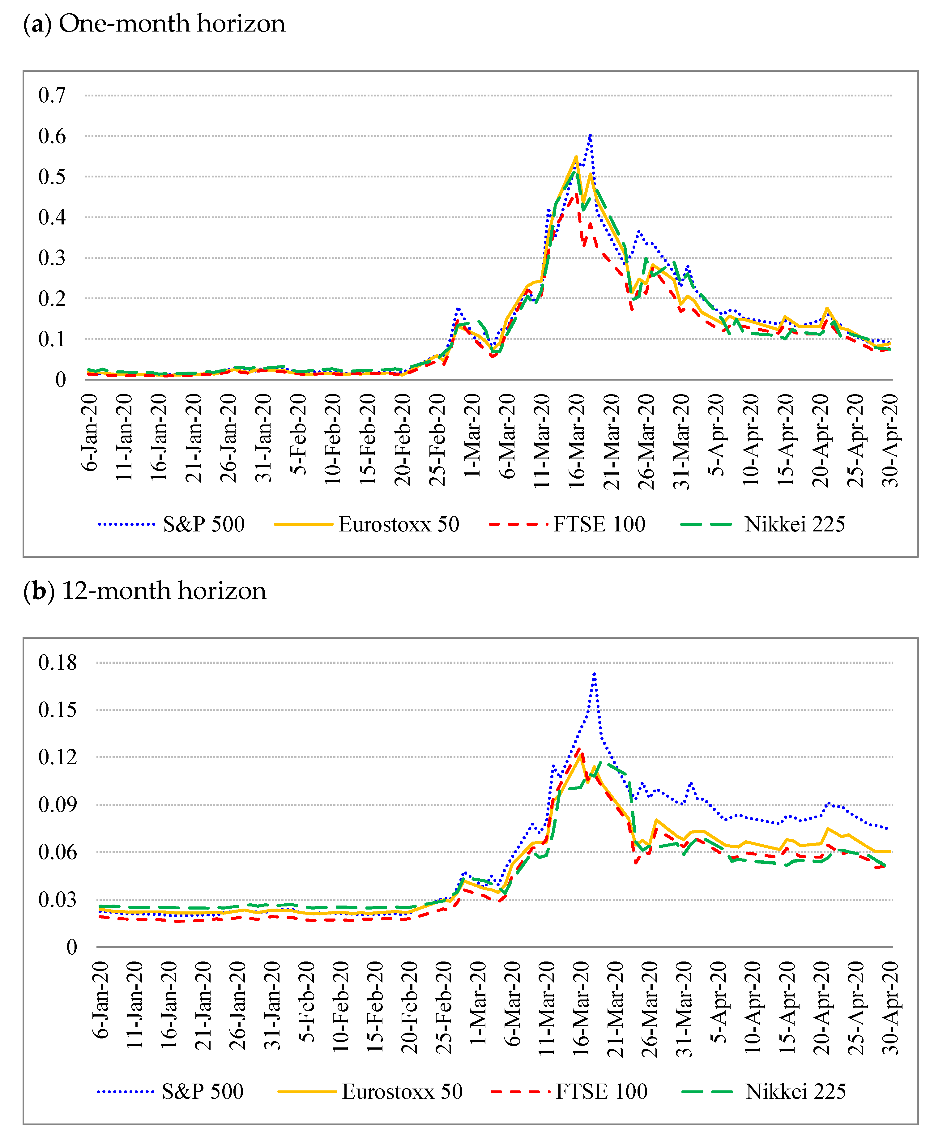
4.2.2. The Time-Varying Behavior of the Expected Market Risk Premia

Figure 7a,b display the expected market risk premia for the one-month and 12-month horizons, respectively, of the four stock markets during the four months corresponding to the Great Recession. Firstly, it is important to point out that the expected market risk premium at the shorter horizon is higher than the expected premium at the longer horizon for the four markets. This is true not only on average, but also during the more distressing days. All estimates follow a well-behaved counter-cyclical pattern, but there are relevant differences across markets. At the shorter horizon, the expected market risk premia of the two European markets and Japan react more deeply than the USA market during the initial days of the crisis. After that, the European countries and the United States follow a similar pattern, with peaks of similar magnitudes while the expected market risk premium of Japan remains above that of the other three markets. In any case, the four markets show a consistent declining pattern for the expected market risk premium from mid-November onwards. In contrast, at the 12-month horizon, the Japanese expected market risk premium remains relatively high even during the final days of the sample period. The declining expected risk premia for the other three markets at the 12-month horizon show smoother decreasing behavior than for the one-month horizon.
Figure 8a,b refer to the COVID-19 subperiod. The two panels emphasize the extraordinary surprise of the pandemic in the four stock markets. There is an initial upward push at the end of February, and a big jump around mid-March. After that, the expected market risk premium for the one-month horizon shows a quick and permanent decline in the four markets. However, the expectations for one-year ahead remain at a relatively high level. Unlike during the Great Recession, Japan is not the country with the consistently highest expected market risk premium. In this case, the USA market has the highest risk premium peaks at the one-month horizon but specially at the 12-month horizon. Therefore, it seems that the stock market in the USA is strongly and negatively influenced by the high uncertainty of the health crisis over a long horizon compared to other markets around the world.
Table 7 reports the average slope of the equity term structure for each stock index during the Great Recession (Panel A) and the COVID-19 crisis (Panel B). The slope is computed as the difference between the expected risk premia for 12-month minus the one-month horizons. In all cases and in both sample periods, the slope is negative on average and is estimated with great precision. The magnitude of the slope during the Great Recession is about double that during the COVID-19. This result is explained by the extraordinarily high expected risk premium at the one-month horizon during the Great Recession. These negative slopes are consistent with the negative average slopes reported in the literature for long sample periods. Confirming the visual conclusion in Figure 7 and Figure 8, Japan reacts more strongly to the Great Recession than the other markets do, whereas the United States is the market most affected by the COVID-19 shock.
Lastly, it is interesting to know whether the (negative) magnitude of the slope is especially high on some specific days with bad stock market results. To investigate this issue, the following OLS regression with heteroskedasticity and autocorrelation consistent standard errors is performed:
E t ( R m 12 ) E t ( R m 1 ) = β 0 + β 1 H N E G t + ε t ,
where E t ( R m 1 ) and E t ( R m 12 ) are the expected risk premia for the one- and 12-month horizons, respectively, and HNEG is a dummy variable that takes the value of one if day t is any of the 15 days with the most negative return during the four months of either the Great Recession or the COVID-19 subperiods, and zero otherwise. The intercept is the average slope outside extreme negative market return days, and the slope is the difference between the average slope on the extreme days and the average slope for the rest of the sample.
Panels A and B of Table 8 report the results for the Great Recession and COVID-19 subperiods, respectively. On average, outside of extreme days, the slopes are higher during the Great Recession than during the COVID-19 pandemic, which is consistent with the evidence reported in Table 7. However, the incremental effects due to extreme bad days become more negative and highly significant during the COVID-19 crisis for all the indexes except for Japan. Indeed, the Japanese stock market does not show any significant incremental effects during either the Great Recession or the health crisis.
Overall, on average, the slope of the term structure of the expected market risk premia between the 12-months and one-month horizons is negative for the four markets and the two crises, but it is higher, in absolute terms, during the financial crisis. Additionally, the slope becomes more negative on extreme bad days in both crises. However, these incremental effects are clearly significant during the COVID-19 crisis. The exogenous nature of the adverse shock of COVID-19 impacts the slope of the expected market risk premia very differently relative to the Great Recession. The response of the expected market risk premia is much stronger during the most critical days of the COVID-19 pandemic.

5. Discussion

This paper analyzes the behavior of the market portfolio return and six popular risk factors during the COVID-19 crisis across a representative set of stock markets around the world. The impact of the pandemic shock on the behavior of the risk factors is a crucial issue given the special importance that distressing economic times have in pricing financial assets. Moreover, the exogenous nature of the adverse shock from COVID-19 presents a unique opportunity for analyzing its effects on stock markets in comparison with the Great Recession. The way in which these factors relate to macroeconomic risks during the two great crises analyzed in this paper shed light on the nature of risks supported by these risk factors.
A relevant economic lesson learnt thorough this research is that it is not appropriate to analyze the performance of risk factors without understanding how market expectations behave. Therefore, in addition to the analysis regarding the past performance of alternative factors, an analysis of the expected market risk premia should be carried out as is the case in this study. One important characteristic of the exogenous shock associated with the pandemic is that expected market risk premia rapidly declined after the outbreak of the COVID-19. However, market expectations during the Great Recession remained in relatively high levels during s much longer time. The underlying nature of any crisis should be considered by institutional investment strategies before deciding how to respond to poor economic times. Value strategies are clear candidates to be big losers when the outbreak of a potential crisis is exogenous as a pandemic or a climate disaster. These types of firms cannot react on time given their large operating leverage. Quality strategies are always defensive against bad economic times, but once again, they will be more valuable when market expectations remain gloomy for a long time relative to an exogenous crisis for which governments and central banks react quickly. Something similar happens with momentum; when the market risk premia show worrying lasting effects, momentum strategies are much more difficult to implement with success. The poor performance of momentum within an endogenous financial crisis takes a long time to recuperate. However, the opposite is true when the origin of the crisis is exogenous with an unexpected and rapid outbreak in which market risk premia tend to return to normal levels in a relatively rapid way. In this case, momentum strategies have a better chance to be a successful style investment strategy.
The key economic message of this research is that the nature of the crisis is a fundamental input to carry out factor investing strategies with promising results.

6. Conclusions

This research evaluates, on the one hand, the performance of systematic risk factors during the first wave of the COVID-19 crisis relative to a comparable long-run pre-COVID period. On the other hand, the effects of the health crisis are compared with those from the economic and financial 2008 crisis by analyzing the evolution of cumulative returns on the risk factors as well as the behavior of expected market risk premia across a selected sample of international indexes.
The study of both risk-adjusted returns and cumulative returns of the risk factors reveals intriguing patterns. While all factors show positive alphas for most of the countries in the pre-COVID period, the three Fama–French factors behave very badly during the COVID crisis, being the value factor the main loser with the exception of the market portfolio. In contrast, during the pandemic, the momentum and quality factors are the winners showing positive CAPM and Fama–French alphas and large cumulative returns for various countries. This performance is probably associated with the fundamentals that drive these investment style strategies. Given that value firms are characterized by having relatively large operating leverage, the negative results for value investing can be explained by the lack of flexibility that these firms face in adapting to new contexts after exogenous crises. Momentum, due to its speculative nature, and quality, due to its hedging property have even been benefited from the pandemic crisis. This study also reports some heterogeneous responses from the risk factors across countries. During the COVID-19 crisis, countries such as Denmark and the Netherlands stand out because of the quality factor’s good performance; Switzerland is unique, with positive and significant risk-adjusted returns for the BAB funding liquidity factor; and the momentum strategy exhibits extraordinary performance for Spain, Great Britain, and Hong Kong.
The comparison between the Great Recession and the pandemic also produces economically relevant results. The cumulative performance of the SMB, HML, and BAB factors is systematically worse during the COVID-19 crisis than through the Great Recession, except for the SMB and BAB factors in Germany. This last result could reflect the German government’s rapid and direct support of small companies and the country’s international financial reputation. In contrast, the cumulative return of the MOM factor is negative during the Great Recession for most countries, but it becomes highly positive in the first three months of 2020. The QMJ factor is the only one that produces positive cumulative returns during both crises and for all countries. Regarding the realized excess market returns, the comparison between the two stressed times shows that losses are much more pronounced during the COVID-19 crisis than during the financial crisis. However, investor expectations about future stock market returns, as reflected in the behavior of option-implied expected market risk premia, and in the slope of their term structure, are more negative and persistent during the Great Recession than during the first wave of the health crisis. These overall results must be nuanced by the behavior of the expected market risk premia during the worst-performing days of the pandemic. Except for Japan, the incremental effects on the slope of the term structure of the expected market risk premia during these extreme days are higher during the COVID-19 crisis than during the Great Recession.
The industry structure and exposure to international trade are relevant facts in potentially explaining the different responses of countries to real activity shocks. Indeed, the main limitation of this research is the lack of direct empirical connections between the financial results of this paper and the real impact of the COVID-19 on the heterogenous industrial sectors across markets. Future research could relate these distinctive aspects of real activity to the responses of stock market returns, risk factors, and expected market risk premia to the COVID-19 pandemic across countries.

Author Contributions

Conceptualization, B.N. and G.R.; methodology, B.N. and G.R.; formal analysis, B.N. and G.R.; investigation, B.N. and G.R.; data curation, B.N.; writing—original draft preparation, G.R.; writing—review and editing, B.N.; funding acquisition, B.N. and G.R. All authors have read and agreed to the published version of the manuscript.

Funding

The authors acknowledge financial support from the Ministry of Science, Innovation, and Universities through grant PGC2018-095072-B-I00. In addition, they acknowledge financial support from Generalitat Valencia grant Prometeo/2017/158.

Institutional Review Board Statement

Not applicable.

Informed Consent Statement

Not applicable.

Data Availability Statement

The data about factor returns are downloaded from AQR Capital Management’s database (www.aqr.com, accessed on 20 May 2020). Options data are from OptionMetrics’ IvyDB Global Indices database.

Acknowledgments

The authors are grateful to the comments and suggestions of the anonymous referees. The views expressed in this paper are those of the authors. Any errors are entirely our own.

Conflicts of Interest

The authors declare no conflict of interest.

Notes

1
Regarding the size effect, see also Alquist et al. (2018).
2
See Asness et al. (2020); Chen and Lu (2019) for additional detailed discussion on the BAB factor and funding liquidity. See Schneider et al. (2020), for a skewness-based explanation of the BAB factor.
3
See Bouchard et al. (2016); González-Urteaga and Rubio (2021) for additional complementary evidence on the QMJ factor.
4
The drop of the Italian GDP during the first quarter of 2020 relative to the previous quarter was 4.8%, while other large European countries like Spain or France experienced higher drops of 5.2% and 5.8%, respectively. It may be explained by the heterogenous effects of the COVID-19 on the different sectors of the economies.
5
With the unique exception of France in the case of the Fama–French risk-adjusted return.
6
Results regarding the other countries are available upon request.
7
This evidence is consistent with the results provided by Ramelli and Wagner (2020), who show that, initially, only firms especially exposed to China underperformed.
8
See Van Binsbergen and Koijen (2017); Bansal et al. (2019); Chabi-Yo and Loudis (2020); Bakshi et al. (2020); Gormsen (2021), for recent evidence on the term structure of the expected market risk premium under alternative procedures and data on either dividend futures or option prices.
9
Rubio et al. (2021), who use the same indexes employed in this paper, find that on average the term structure of expected market risk premia is slightly downward sloping, but, more importantly, it becomes highly downward sloping in bad economic times.

References

  1. Alquist, Ron, Ronen Israel, and Tobias J. Moskowitz. 2018. Fact, Fiction, and the Size Effect. The Journal of Portfolio Management 45: 3–30. [Google Scholar] [CrossRef]
  2. Ampudia, Miguel, Ursel Baumann, and Fabio Fornari. 2020. Coronavirus (COVID-19): Market Fear as Implied by Options Prices. ECB Economic Bulletin 4: 1–9. Available online: https://www.ecb.europa.eu/pub/economic-bulletin/focus/2020/html/ecb.ebbox202004_02~26672a3808.en.html (accessed on 15 July 2021).
  3. Asness, Cliffor S., Andrea Frazzini, Ronen Israel, and Tobias J. Moskowitz. 2015a. Fact, Fiction, and Momentum Investing. The Journal of Portfolio Management 40: 75–92. [Google Scholar] [CrossRef]
  4. Asness, Clifford S., Andrea Frazzini, Ronen Israel, and Tobias J. Moskowitz. 2015b. Fact, Fiction, and Value Investing. The Journal of Portfolio Management 42: 34–52. [Google Scholar] [CrossRef]
  5. Asness, Clifford S., and Andrea Frazzini. 2013. The Devil in HML’s Details. The Journal of Portfolio Management 39: 49–68. [Google Scholar] [CrossRef]
  6. Asness, Clifford S., Andrea Frazzini, and Lasse H. Pedersen. 2019. Quality Minus Junk. Review of Accounting Studies 24: 34–112. [Google Scholar] [CrossRef] [Green Version]
  7. Asness, Clifford S., Andrea Frazzini, Niels J. Gormsen, and Lasse H. Pedersen. 2020. Betting against Correlation: Testing Theories of the Low-Risk Effect. Journal of Financial Economics 135: 629–52. [Google Scholar] [CrossRef]
  8. Asness, Clifford S., Andrea Frazzini, Ronen Israel, Tobias J. Moskowitz, and Lasse H. Pedersen. 2018. Size Matters if you Control your Junk. Journal of Financial Economics 129: 479–509. [Google Scholar] [CrossRef]
  9. Asness, Clifford S., Antti Ilmanen, Ronen Israel, and Tobias J. Moskowitz. 2015c. Investing with Style. Journal of Investment Management 13: 27–63. [Google Scholar]
  10. Asness, Clifford S., Tobias J. Moskowitz, and Lasse H. Pedersen. 2013. Value and Momentum Everywhere. The Journal of Finance 68: 929–85. [Google Scholar] [CrossRef] [Green Version]
  11. Baker, Scott R., Nicholas Bloom, Steven J. Davis, Kyle Kost, Macro Sammon, and Tasaneeya Viratyosin. 2020. The Unprecedent Stock Market Reaction to COVID-19. The Review of Asset Pricing Studies 10: 742–58. [Google Scholar] [CrossRef]
  12. Bakshi, Gurdip, John Crosby, Xiaohui Gao, and Wei Zhou. 2020. A New Formula for the Expected Excess Return of the Market. Available online: https://ssrn.com/abstract=3464298 (accessed on 30 January 2021).
  13. Bansal, Ravi, Shane Miller, Dongho Song, and Amir Yaron. 2019. The Term Structure of Equity Risk Premia. NBER. Working Paper 25690. Available online: https://www.nber.org/papers/w25690 (accessed on 4 June 2019).
  14. Bouchard, Jean-Philippe, Stefano Ciliberti, Augustin Landier, Guillaume Simon, and David Thesmar. 2016. The Excess Returns of “Quality” Stocks: A Behavioral Anomaly. Journal of Investing Strategies 5: 51–61. [Google Scholar] [CrossRef] [Green Version]
  15. Bretscher, Lorenzo, Alex Hsu, Peter Simasek, and Andrea Tamoni. 2020. COVID-19 and the Cross-Section of Equity Returns: Impact and Transmission. The Review of Asset Pricing Studies 10: 705–41. [Google Scholar] [CrossRef]
  16. Carhart, Mark M. 1997. On Persistence in Mutual Fund Performance. The Journal of Finance 52: 57–82. [Google Scholar] [CrossRef]
  17. Chabi-Yo, Fousseni, and Johnathan Loudis. 2020. The Conditional Expected Market Return. Journal of Financial Economics 137: 752–86. [Google Scholar] [CrossRef]
  18. Chen, Zhuo, and Andrea Lu. 2019. A Market-Based Funding Liquidity Measure. The Review of Asset Pricing Studies 9: 356–93. [Google Scholar] [CrossRef]
  19. Clarke, Charles. 2021. The Level, Slope, and Curve Factor Models for Stocks. Journal of Financial Economics 143: 159–87. [Google Scholar] [CrossRef]
  20. Cochrane, John H. 2011. Presidential Address: Discount Rates. The Journal of Finance 66: 1047–108. [Google Scholar] [CrossRef] [Green Version]
  21. Fama, Eugene F., and Kenneth R. French. 1993. Common Risk Factors in the Return of Stocks and Bonds. Journal of Financial Economics 33: 3–56. [Google Scholar] [CrossRef]
  22. Frazzini, Andrea, and Lasse H. Pedersen. 2014. Betting against Beta. Journal of Financial Economics 111: 1–25. [Google Scholar] [CrossRef] [Green Version]
  23. González-Sánchez, Mariano, Juan Nave, and Gonzalo Rubio. 2018. Macroeconomic Determinants of Stock Market Betas. Journal of Empirical Finance 45: 26–44. [Google Scholar] [CrossRef]
  24. González-Sánchez, Mariano, Juan Nave, and Gonzalo Rubio. 2020. Effects of Uncertainty and Risk Aversion on the Exposure of Investment-Style Factor Returns to Real Activity. Research in International Business and Finance 53: 583–96. [Google Scholar] [CrossRef]
  25. González-Urteaga, Ana, and Gonzalo Rubio. 2021. The Quality Premium with Leverage and Liquidity Constraints. International Review of Financial Analysis 75: 101699. [Google Scholar] [CrossRef]
  26. Gormsen, Niels J. 2021. Time Variation of the Equity Term Structure. The Journal of Finance 76: 1959–99. [Google Scholar] [CrossRef]
  27. Gormsen, Niels J., and Ralph S. J. Koijen. 2020. Coronavirus: Impact on Stock Prices and Growth Expectations. The Review of Asset Pricing Studies 10: 574–97. [Google Scholar] [CrossRef]
  28. Harvey, Campbell R., Yan Liu, and Heqing Zhu. 2016. … and the Cross-Section of Expected Returns. The Review of Financial Studies 29: 5–68. [Google Scholar] [CrossRef] [Green Version]
  29. Israel, Ronen, and Thomas Maloney. 2014. Understanding Style Premia. The Journal of Investing 23: 15–22. [Google Scholar] [CrossRef]
  30. Israel, Ronen, Kristoffer Lauren, and Scott Richardson. 2021. Is (Systematic) Value Investing Dead? The Journal of Portfolio Management 47: 38–62. [Google Scholar] [CrossRef]
  31. Jackwerth, Jens. 2020. What Do Index Options Teach US About COVID-19? The Review of Asset Pricing Studies 10: 618–34. [Google Scholar] [CrossRef]
  32. Jensen, Theis I., Bryan T. Kelly, and Lasse H. Pedersen. 2021. Is There a Replication Crisis in Finance? NBER Working Paper 28432. Available online: https://www.nber.org/papers/w28432 (accessed on 10 May 2021).
  33. Kelly, Bryan T., Tobias J. Moskowitz, and Seth Pruitt. 2021. Understanding Momentum and Reversal. Journal of Financial Economics 140: 726–43. [Google Scholar] [CrossRef]
  34. Maio, Paulo, and Dennis Philip. 2018. Economic Activity and Momentum Profits: Further Evidence. Journal of Banking and Finance 88: 466–82. [Google Scholar] [CrossRef] [Green Version]
  35. Martin, Ian. 2017. What is the Expected Return on the Market? The Quarterly Journal of Economics 132: 367–433. [Google Scholar] [CrossRef] [Green Version]
  36. Ramelli, Stefano, and Alexander F. Wagner. 2020. Feverish Stock Price Reactions to COVID-19. The Review of Corporate Finance Studies 9: 622–55. [Google Scholar] [CrossRef]
  37. Rossi, Alberto G., and Allan Timmermann. 2015. Modelling Covariance Risk in Merton’s ICAPM. The Review of Financial Studies 28: 1428–61. [Google Scholar] [CrossRef] [Green Version]
  38. Rubio, Gonzalo, Pedro Serrano, and Antoni Vaello. 2021. University CEU Cardenal Herrera, Elche, Sapin, University Carlos III, Madrid, Spain, University Islas Baleares, Mallorca, Sapin. The Term Structure of International Option-Implied Expected Equity Risk Premia and its Reaction to Uncertainty and Risk Aversion Shocks. Personal communication. [Google Scholar]
  39. Schneider, Paul, Christian Wagner, and Josef Zechner. 2020. Low Risk Anomalies? The Journal of Finance 75: 2673–718. [Google Scholar] [CrossRef] [Green Version]
  40. Spatt, Chester S. 2020. A Tale of Two Crises: The 2008 Mortgage Meltdown and the 2020 COVID-19 Crisis. The Review of Asset Pricing Studies 10: 759–90. [Google Scholar] [CrossRef]
  41. Van Binsbergen, Jules H., and Ralph S. J. Koijen. 2017. The Term Structure of Returns: Facts and Theory. Journal of Financial Economics 124: 1–21. [Google Scholar] [CrossRef] [Green Version]
  42. Zhang, Lu. 2005. The Value Premium. The Journal of Finance 60: 67–103. [Google Scholar] [CrossRef]
Figure 1. t-Statistics for the CAPM Alphas for the Risk Factors: Global Index. This figure displays the t-statistics for testing the significance of the intercept from a regression of each alternative risk factor on the excess market return for the global international stock market index. See notes in Table 1 for the definition of the factos. (a) shows the results when using monthly data for the first quarter of each of the years between 1997 and 2019, and (b) shows the results when using daily data for the subperiod affected by the first impact of the COVID-19 pandemic from January to March 2020.
Jrfm 15 00013 g001
Figure 2. t-Statistics for the CAPM Alphas for the Risk Factors: By Country. This figure displays the t-statistics for testing the significance of the intercept from a regression of each alternative risk factor on the excess market returns for representative stock markets around the world. See notes in Table 1 for the definition of the factors and the countries. (a) shows the results when using monthly data for the first quarter of each of the years between 1997 and 2019, and (b) shows the results when using daily data for the subperiod affected by the first impact of the COVID-19 pandemic from January to March 2020.
Jrfm 15 00013 g002
Figure 3. t-Statistics for the Fama–French Alphas for the Other Risk Factors: Global Index. This figure displays t-statistics for testing the significance of the intercept from a regression of either the momentum factor (MOM), the quality factor (QMJ), or the betting-against-beta factor (BAB) on the three factors of the Fama–French (1993) model for the global international stock market index. (a) shows the results when using monthly data for the first quarter of each of the years between 1997 and 2019. (b) shows the results when using daily data for the subperiod affected by the first impact of the COVID-19 pandemic from January to March 2020.
Jrfm 15 00013 g003
Figure 4. t-Statistics for the Fama–French Alphas for the Other Risk Factors: By Country. This figure displays t-statistics for testing the significance of the intercept from a regression of either the momentum factor (MOM), the quality factor (QMJ), or the betting-against-beta factor (BAB) on the three factors of the Fama–French (1993) model for representative stock markets around the world. See notes in Table 1. (a) shows the results when using monthly data for the first quarter of each of the years between 1997 and 2019, and (b) shows the results when using daily data for the subperiod affected by the first impact of the COVID-19 pandemic from January to March 2020.
Jrfm 15 00013 g004
Figure 5. Cumulative Returns: Global Index. This figure displays the time series behavior of the cumulative returns of the different risk factors along two subsample periods: The Great Recession (a) and the COVID-19 crisis (b). See notes in Table 1 for the definition of the factors.
Jrfm 15 00013 g005aJrfm 15 00013 g005b
Figure 6. Cumulative Returns: By Country. This figure displays the time series behavior of the cumulative return of the different risk factors along two subsample periods: The Great Recession (a1a6) and the COVID-19 crisis (b1b6). The factors refer to different stock markets around the world: The United States (1), Germany (2), Great Britain (3), Australia (4), Hong Kong (5), and Japan (6). See notes in Table 1 for the definition of the factors.
Jrfm 15 00013 g006aJrfm 15 00013 g006bJrfm 15 00013 g006cJrfm 15 00013 g006dJrfm 15 00013 g006e
Figure 7. Expected Market Risk Premia: The Great Recession. This figure displays the time series behavior of the expected market risk premia estimated from option prices with four alternative underlying stock indexes: the S&P 500, Euro Stoxx 50, Nikkei 225, and FTSE 100. The expected risk premia are estimated daily following Martin (2017) and using options with maturities of one month (a) and 12 months (b). The sample period comprises the four months with the worst stock market results during the Great Recession from September 2008 to December 2008.
Jrfm 15 00013 g007
Figure 8. Expected Market Risk Premia: COVID-19 Crisis. This figure displays the time series behavior of the expected market risk premia estimated from option prices with four alternative underlying stock indexes: the S&P 500, Euro Stoxx 50, Nikkei 225, and FTSE 100. The expected risk premia are estimated daily following Martin (2017) and using options with maturities of one month (a) and 12 months (b). The sample period refers to the first wave of the COVID-19 pandemic and goes from January to April 2020.
Jrfm 15 00013 g008
Table 1. Annualized Average Returns.
Panel A: Pre-COVID-19Panel B: COVID-19
January through March for All Years 1997–2019January through March 2020
MKTSMBHMLHML DMOMQMJBABMKTSMBHMLHML DMOMQMJBAB
SWI0.0540.0860.0890.0140.1840.0550.131−0.536−0.240−0.362−0.5590.2790.3071.959
DEU0.0560.0450.020−0.0160.1850.0350.054−0.9690.146−0.495−0.6410.3480.1160.380
DNK0.1710.050−0.028−0.0500.0330.0590.125−0.3420.032−0.591−1.0630.5980.8390.151
SPN0.0550.2200.0770.0470.0170.0030.118−1.190−0.0290.171−0.1840.8820.2140.334
FRA0.0720.0720.045−0.0030.108−0.0030.214−1.1050.009−0.374−0.4150.2100.5650.205
GBR0.0220.0590.0530.0430.1360.0780.092−1.276−0.302−0.526−0.7960.5810.180−0.103
ITA0.0940.1080.1180.0070.1240.0680.161−1.137−0.185−0.376−0.6930.6180.369−0.063
NLD0.0650.1300.0170.0020.1290.0480.111−0.785−0.239−0.184−0.3500.7011.0160.002
AUS0.104−0.0180.1120.0130.2460.0510.118−1.493−0.196−0.468−0.5060.5580.429−0.291
JPN0.0530.0770.0710.163−0.065−0.0210.030−0.669−0.106−0.083−0.1560.1700.236−0.067
HKG0.0330.1320.0110.0140.1900.0780.282−0.5060.019−0.469−0.5160.5210.097−0.402
USA0.0770.0470.0020.0230.0630.0060.137−0.793−0.394−0.912−1.0550.5520.182−0.272
Global0.0640.0580.0350.0430.0800.0180.131−0.936−0.265−0.674−0.8070.5250.239−0.212
Notes: This table shows average returns (on an annual basis) of a set of systematic risk factors for 12 different stock markets around the world and an international global index. The countries, indicated in the first column, are: Switzerland (SWI), Germany (DEU), Denmark (DNK), Spain (SPN), France (FRA), Great Britain (GBR), Italy (ITA), and Netherlands (NLD) from Europe, Australia (AUS) from Oceania, Japan (JPN) and Hong Kong (HKG) from Asia, and United States (USA) from North America. In Panel A, the average returns are computed using the first three months of each of the years from 1997 through 2019, namely, the pre-COVID period. In Panel B, the average returns refer to the period of the first wave of the COVID-19 pandemic, that is, the first quarter of 2020. The risk factors are the excess market return (MKT); the size factor (SMB); the Fama and French (1993) value-growth factor (HML); the HML devil proposed by AQR Capital Management with monthly price updates in the book-to-market ratio (HML D); the momentum factor (MOM) of Carhart (1997), which is the return differential between winners and losers using the returns of the previous two to 12 months; the quality factor (QMJ), which is the return differential between high- and junk-quality firms, as defined by Asness et al. (2019); and the betting against beta (BAB) factor of Frazzini and Pedersen (2014), which is the return differential between leveraged low-beta stocks and de-leveraged high-beta stocks. The HMLs, MOM, and QMJ factors are controlled for size, and the SMB factor is controlled for value and growth. All returns are in USA dollars.
Table 2. Annualized Volatilities.
Panel A: Pre-COVID-19Panel B: COVID-19
January through March for All Years 1997–2019January through March 2020
MKTSMBHMLHML DMOMQMJBABMKTSMBHMLHML DMOMQMJBAB
SWI0.1590.0930.1040.1100.1230.1120.1620.2870.1060.1180.1220.1640.1480.363
DEU0.1870.1150.1060.1200.1330.0920.1970.3270.0930.1130.1250.0890.0740.327
DNK0.1690.1260.1540.1580.1440.1290.1730.2940.1510.1660.1780.1240.1290.163
SPN0.2060.1100.1170.1290.1450.1320.1790.3560.1410.1470.1370.1310.1740.257
FRA0.1850.1160.0940.1030.1180.0940.1660.3580.1460.1040.1040.0860.1040.213
GBR0.1670.1140.0900.0970.1110.0800.1090.3700.1730.1340.1490.1040.0610.146
ITA0.2080.1170.1160.1260.1480.1260.1410.4160.1590.1180.1330.1080.1070.134
NLD0.1820.1140.1350.1510.1660.1450.1830.3290.1250.1320.1850.1650.1660.244
AUS0.1740.0980.0820.0980.1030.0750.1030.3860.2120.1160.1300.1010.1120.151
JPN0.2090.0860.0670.0880.1270.0880.1450.2530.0990.0880.1010.0660.0480.147
HKG0.2110.1260.1100.1160.1290.1130.1380.2950.1370.0920.0930.0710.0620.070
USA0.1580.0740.0710.0920.1190.0720.0940.4270.1140.1140.1380.1140.0870.223
Global0.1250.0490.0460.0610.0860.0530.0690.3310.0710.0750.0910.0740.0590.139
Notes: This table shows the standard deviation (on an annual basis) of the daily returns of a set of systematic risk factors for 12 different stock markets around the world and an international global index. See notes in Table 1.
Table 3. Sharpe Ratios.
Panel A: Pre-COVID-19Panel B: COVID-19
January through March for All Years 1997–2019January through March 2020
MKTSMBHMLHML DMOMQMJBABMKTSMBHMLHML DMOMQMJBAB
SWI0.2820.2800.2760.0710.5420.0650.191−0.596−0.548−0.654−0.6530.6740.6530.789
DEU0.2290.2140.085−0.0560.4890.1300.042−1.0130.527−1.100−1.3710.9430.2130.568
DNK0.4170.1680.053−0.0550.1660.1630.293−0.3320.766−1.054−1.7141.2471.9320.423
SPN0.2000.6620.2040.0900.1410.0410.263−0.9860.1140.349−0.4101.9760.2070.263
FRA0.2670.2630.201−0.0060.438−0.0140.374−1.056−0.041−0.907−1.0440.8561.1780.370
GBR0.1980.2480.1730.0350.6500.3270.469−1.251−0.206−1.122−1.4701.8890.7340.040
ITA0.2600.3000.2970.0310.3620.2080.345−0.739−0.492−0.730−1.2841.8590.762−0.152
NLD0.2830.3970.047−0.0500.3180.1380.296−0.7660.124−0.686−0.6941.3631.8910.028
AUS0.240−0.0500.4490.0340.8980.2260.409−0.948−0.504−1.227−1.3561.4980.906−0.347
JPN0.1520.3300.4030.5200.2190.0260.136−1.016−0.843−0.161−0.3330.7041.9150.174
HKG0.1900.3120.0570.0020.6120.4100.714−0.4690.089−1.395−1.5562.2350.352−1.414
USA0.3700.2370.0100.0260.4030.0330.807−0.617−0.978−2.637−2.6081.638−0.024−0.086
Global0.3530.4410.2920.1750.6070.1450.891−0.893−1.006−2.807−2.8642.2260.535−0.050
Notes: This table shows the Sharpe ratios of a set of systematic risk factors for 12 different stock markets around the world and an international global index. See notes in Table 1.
Table 4. Annualized CAPM Alphas.
Panel A: Pre-COVID-19Panel B: COVID-19
January through March for All Years 1997–2019January through March 2020
SMBHMLHML DMOMQMJBABSMBHMLHML DMOMQMJBAB
SWI0.0960.0970.0070.1950.0770.140−0.320−0.378−0.5410.2770.2591.957
(2.10)(2.10)(0.14)(3.44)(1.69)(2.61)(−1.47)(−1.52)(−1.88)(0.75)(0.80)(2.09)
DEU0.0520.023−0.0100.2040.0510.063−0.001−0.372−0.5620.3990.0410.204
(1.19)(0.38))(−0.13)(2.89)(1.61)(1.01)(−0.01)(−1.67)(−2.18)(2.16)(0.29)(0.31)
DNK0.061−0.011−0.0280.0380.0720.135−0.026−0.589−1.0590.6350.8040.144
(1.04)(−0.18)(−0.42)(0.63)(1.45)(1.58)(−0.08)(−1.69)(−2.69)(2.51)(3.12)(0.42)
SPN0.2210.0770.0480.0290.0230.116−0.2430.332−0.1570.845−0.018−0.101
(4.59)(1.28)(0.79)(0.40)(0.45)(1.60)(−0.92)(1.16)(−0.56)(3.00)(−0.05)(−0.23)
FRA0.0820.0580.0080.1210.0180.222−0.317−0.348−0.3950.1840.401−0.073
(1.87)(0.92)(0.10)(2.01)(0.42)(3.42)(−1.34)(−1.51)(−1.73)(1.02)(2.02)(−0.19)
GBR0.0630.0510.0390.1450.0820.093−0.464−0.380−0.6410.6070.135−0.045
(1.19)(0.99)(0.63)(2.08)(2.74)(1.48)(−1.15)(−1.28)(−1.88)(2.62)(1.08)(−0.14)
ITA0.0920.098−0.0080.1430.1060.157−0.468−0.300−0.6310.6550.263−0.046
(2.01)(2.14)(−0.11)(1.75)(1.65)(2.14)(−1.88)(−1.19)(−2.17)(2.86)(1.21)(−0.17)
NLD0.1280.017−0.0230.1580.0760.116−0.232−0.251−0.4780.7090.768−0.213
(2.95)(0.29)(−0.36)(2.05)(1.23)(1.70)(−0.82)(−0.91)(−1.23)(1.94)(2.48)(−0.46)
AUS−0.0070.1150.0080.2670.0650.101−0.619−0.519−0.6560.6050.261−0.293
(−0.15)(2.34)(0.16)(4.83)(1.86)(2.17)(−1.37)(−2.13)(−2.52)(2.79)(1.09)(−0.83)
JPN0.0740.0710.158−0.052−0.0020.027−0.082−0.113−0.1820.1890.1760.073
(2.35)(2.09)(2.89)(−0.69)(−0.06)(0.46)(−0.35)(−0.61)(−0.87)(1.43)(1.76)(0.22)
HKG0.1300.0090.0130.1990.1000.291−0.191−0.441−0.5020.5480.078−0.393
(1.85)(0.13)(0.16)(2.44)(1.27)(2.72)(−1.74)(−2.38)(−2.67)(3.92)(0.64)(−2.83)
USA0.0420.0130.0170.0950.0340.168−0.458−0.895−1.0470.6030.1700.018
(0.99)(0.28)(0.29)(1.28)(1.00)(2.76)(−1.74)(−3.51)(−3.38)(2.59)(0.83)(0.05)
Global0.0580.0430.0420.1020.0400.147−0.347−0.635−0.7860.5310.1690.068
(1.94)(1.20)(0.86)(1.71)(1.77)(3.75)(−2.32)(−3.77)(−3.79)(3.34)(1.28)(0.28)
Notes: This table displays the CAPM alphas (annualized) and their correspondent t-statistics for a set of systematic risk factors for 12 different stock markets around the world and an international global index. See notes in Table 1. Panel A uses monthly returns, and the sample period comprises the first three months of each of the years from 1997 through 2019, namely, the pre-COVID period. Panel B uses daily returns within the period of the first wave of the COVID-19 pandemic: the first quarter of 2020.
Table 5. Annualized Fama–French Alphas.
Panel A: Pre-COVID-19Panel B: COVID-19
January through March for All Years 1997–2019January through March 2020
MOMQMJBABMOMQMJBAB
SWI0.1610.1180.0950.0930.1212.223
(2.63)(2.46)(1.67)(0.25)(0.37)(2.30)
DEU0.2010.0590.0760.252−0.0580.271
(2.86)(1.91)(1.22)(1.58)(−0.44)(0.40)
DNK0.0420.0920.1200.4770.5060.225
(0.68)(2.06)(1.41)(2.02)(2.39)(0.64)
SPN0.0990.1540.1540.807−0.004−0.006
(1.19)(3.16)(1.87)(2.82)(−0.01)(−0.01)
FRA0.1530.0590.184−0.0100.125−0.277
(2.51)(1.55)(2.87)(−0.07)(0.79)(−0.72)
GBR0.1590.1050.0440.5380.0640.026
(2.26)(3.70)(0.74)(3.20)(0.51)(0.10)
ITA0.0820.1170.0690.4190.013−0.027
(0.98)(1.76)(0.97)(1.84)(0.06)(−0.09)
NLD0.1860.1480.1270.4120.541−0.077
(2.27)(2.44)(1.73)(1.45)(2.10)(−0.17)
AUS0.2730.0700.0890.329−0.075−0.147
(4.69)(2.01)(1.84)(1.70)(−0.39)(−0.49)
JPN−0.1070.0420.0130.1400.1580.099
(−1.37)(1.29)(0.20)(1.44)(1.69)(0.30)
HKG0.2020.1710.2200.342−0.106−0.271
(2.46)(2.69)(2.40)(2.92)(−0.98)(−1.93)
USA0.0900.0540.1760.003−0.2320.132
(1.18)(2.06)(3.35)(0.02)(−1.28)(0.35)
Global0.0750.0670.1260.079−0.1590.115
(1.19)(3.58)(3.78)(0.66)(−1.36)(0.43)
Notes: This table displays the Fama–French alphas (annualized) and their correspondent t-statistics for the momentum factor (MOM), the quality factor (QMJ), and the betting against beta factor (BAB) for 12 different stock markets around the world and an international global index. See notes in Table 1. Panel A uses monthly returns, and the sample period comprises the first three months of each of the years from 1997 through 2019, namely, the pre-COVID period. Panel B uses daily returns within the period of the first wave of the COVID-19 pandemic: the first quarter of 2020.
Table 6. Annualized Minimum Cumulative Return.
Panel A: The Great Recession
October 2007–August 2009
MKTSMBHMLHML DMOMQMJBAB
DEU−29.53 −2.46 0.53 15.52 10.74 20.98 −4.66
GBR−35.68 −21.00 5.73 14.70 −5.50 12.87 −55.74
AUS−34.21 −7.89 5.69 2.07 3.31 16.73 −7.27
JPN−21.86 −4.47 7.14 22.81 −15.79 4.98 −1.41
HKG−24.75 −1.52 −1.64 18.10 −46.53 11.32 −9.84
USA−27.70 2.40 −10.71 0.01 −25.36 15.22 −23.81
Global−28.46 −3.30 −3.80 7.62 −16.58 13.00 −16.10
Panel B: COVID-19
January 2020–March 2020
MKTSMBHMLHML DMOMQMJBAB
DEU−196.83 24.99 −45.24 −56.99 25.14 9.42 60.94
GBR−258.10 −18.49 −59.47 −83.92 53.42 10.74 −31.25
AUS−273.80 −27.96 −42.34 −41.16 57.36 58.96 −49.71
JPN−147.13 −20.18 −5.97 −13.89 12.02 27.83 −21.03
HKG−109.51 28.19 −60.63 −61.18 50.79 11.74 −51.14
USA−179.23 −34.62 −104.89 −116.09 55.67 21.52 −72.59
Global−179.23 −18.19 −76.81 −88.32 49.60 26.19 −41.30
Notes: Assuming an investment of 1 dollar at the beginning of the period, this table shows the minimum cumulative return (on an annual basis and percent) for each systematic risk factor and for six different stock markets around the world, and the international global index. See notes in Table 1. In Panel A, the period is the Great Recession, from 1 October 2007 to 31 August 2009. In Panel B, the period is the first wave of the COVID-19 crisis, that is, the first quarter of 2020.
Table 7. Average Slope of the Term Structure of the Expected Market Risk Premia.
Panel A: The Great Recession
September 2008–December 2008
S&P 500Euro Stoxx 50Nikkei 225FTSE 100
−0.140−0.144−0.186−0.133
(−6.69)(−6.15)(−4.98)(−6.32)
Panel B: COVID-19
January 2020–April 2020
S&P 500Euro Stoxx 50Nikkei 225FTSE 100
−0.075−0.074−0.074−0.061
(−3.25)(−3.22)(−3.37)(−3.46)
Notes: This table reports the average slopes of the term structure of the expected risk premia estimated from option prices with four alternative underlying stock indexes: The S&P 500, Euro Stoxx 50, Nikkei 225, and FTSE 100. The expected risk premia are estimated daily following Martin (2017) and using option prices with maturities of one and 12 months. The slope of the term structure is the difference between them. In Panel A, the sample period comprises the four months during the Great Recession with the worst stock market results, from September 2008 to December 2008. In Panel B, the results refer to the first wave of the COVID-19 pandemic, and the sample period goes from January 2020 to April 2020. The t-statistics are in parentheses.
Table 8. Conditional Average Slopes of the Term Structure of the Expected Market Risk Premia.
Panel A: The Great Recession
September 2008–December 2008
S&P 500Euro Stoxx 50Nikkei 225FTSE 100
Intercept−0.128−0.122−0.171−0.115
(−6.74)(−6.67)(−4.74)(−6.52)
Slope−0.052−0.090−0.063−0.075
(−1.57)(−2.42)(−1.49)(−1.81)
Adj. R2 (%) 3.369.170.787.04
Panel B: COVID-19
January 2020–April 2020
S&P 500Euro Stoxx 50Nikkei 225FTSE 100
Intercept−0.052−0.051−0.065−0.039
(−2.91)(−2.90)(−2.82)(−4.35)
Slope−0.112−0.107−0.045−0.101
(−3.16)(−3.55)(−1.46)(−5.17)
Adj. R2 (%) 17.0517.102.1025.78
Notes: This table displays the differential average slope of the term structure of the equity risk premia for the most distressing 15 days within each subsample: from September 2008 to December 2008 for the Great Recession (Panel A) and from January to April 2020 for the COVID-19 health crisis (Panel B). The expected risk premia are estimated daily following Martin (2017) and using option prices with maturities of one and 12 months. The slope of the term structure is the difference between them. The underlying stock indexes are selected to represent different international geographical areas and are the S&P 500, Euro Stoxx 50, Nikkei 225, and FTSE 100. The slope is regressed on a constant, and the dummy variable that takes the value of one if the day is any of the 15 days with the most negative stock market return during the four months of each subperiod and zero otherwise. The table reports the estimates and R-squared (in percent), and t-statistics in parentheses computed with heteroskedasticity- and autocorrelation-consistent standard errors.
Publisher’s Note: MDPI stays neutral with regard to jurisdictional claims in published maps and institutional affiliations.

