
A Reappraisal of the Prebisch-Singer Hypothesis Using Wavelets Analysis


School of Business, Faculty of Management, Royal Roads University, Victoria, BC V9B 5 Y2, Canada
J. Risk Financial Manag. 2021, 14(7), 319; https://doi.org/10.3390/jrfm14070319
Submission received: 8 May 2021
/
Revised: 15 June 2021
/
Accepted: 24 June 2021
/
Published: 12 July 2021
(This article belongs to the Special Issue Financial and Panel Data Econometrics)
Abstract
:The Prebisch-Singer (PS) hypothesis, which postulates the presence of a downward secular trend in the price of primary commodities relative to manufacturers, remains at the core of a continuing debate among international trade economists. The reason is that the results of testing the PS hypothesis depend on the starting point of the technical analysis, i.e., stationarity, nonlinearity, and the existence of structural breaks. The objective of this paper is to appraise the PS hypothesis in the short- and long-run by employing a novel multiresolution wavelets decomposition to a unique data set of commodity prices. The paper also seeks to assess the impact of the terms of trade (also known as Incoterms) on the test results. The analysis reveals that the PS hypothesis is not supported in the long run for the aggregate commodity price index and for most of the individual commodity price series forming it. Furthermore, in addition to the starting point of the analysis, the results show that the PS test depends on the term of trade classification of commodity prices. These findings are of particular significance to international trade regulators and policymakers of developing economies that depend mainly on primary commodities in their exports.
1. Introduction
The hypothesis that the price of primary commodities relative to those of manufacturers presents a downward secular trend (Prebisch 1950; Singer 1950), or the Prebisch-Singer (PS) hypothesis, is central for least developed economies that specialize in producing and exporting primary products while importing manufacturers. The hypothesis, which is independently posed by Prebisch (1950) and Singer (1950), asserts that such specialization causes a steady decline in the economy’s net barter terms of trade and, hence, the real income of the country. It is, therefore, important for policymakers to assess the empirical validity of this hypothesis as the decision to accept or to reject the hypothesis can have profound policy implications. For instance, strong evidence supporting a long-run downward trend in a country’s key primary exports might lead to a change in policy or a restructure in the country’s export portfolio to include manufacturers and services.
To this day, the PS hypothesis remains at the core of a continuing debate among policymakers and international trade economists. The main reason for the sustained interest in the topic is that the fundamental question implied by the PS hypothesis is impossible to answer without turning to data (Balagtas and Holt 2009). The answer, however, varies according to the starting point of the analysis, i.e., the statistical/technical properties of the price series, and other non-technical factors, such as commodity classifications and aggregations. While the statistical properties of the price series have been extensively discussed in the literature, studying the impact of other non-technical factors remains a fruitful research area. The empirical literature on the subject uses various techniques to test the PS hypothesis and the consensus is that the result whether to accept or reject the hypothesis depends on the starting point of the analysis, i.e., the stationarity of the data generating process (Ardeni and Wright 1992; Bleaney and Greenaway 1993; Cuddington and Urzua 1989; Grilli and Yang 1988; Harvey et al. 2010; Helg 1991; Lutz 1999; Newbold and Vougas 1996; Powell 1991; Sapsford 1985; Spraos 1980; Thirlwall and Bergevin 1985; Trivedi 1995), nonlinearity (Balagtas and Holt 2009; Persson and Teräsvirta 2003), and the existence of structural breaks (Cuddington and Urzua 1989; Kellard and Wohar 2006; Leon and Soto 1997; Newbold and Vougas 1996; Zanias 2005).
In addition to stationarity, nonlinearity, and the existence of structural breaks, Fahmy (2011, 2014, 2017) shows that the terms of trade, i.e., the international sales terms of commodity prices (also known as border prices or Incoterms) contain significant information that contribute to our understanding of the behavior of the price series. The author shows that nonlinear free on board (FOB) and cost insurance and freight (CIF) real commodity prices that are driven by exogenous regime-driving macroeconomic variables, e.g., inflation and oil price, do not display downward trends because the fluctuations in the exogenous regime-driving variables impact their nonlinear behavior. Thus, the PS hypothesis is unlikely to be supported for this type of border prices.
The objective of this paper is to re-examine the PS hypothesis by employing a novel multiresolution wavelets decomposition to the Grilli and Yang (1988) data set. The intention is to separate the real price series into time and scale components and to test the PS hypothesis in the short- and long-run using a bivariate co-integration framework. Furthermore, the paper seeks to assess whether the results of the analysis depend on the information contained in the terms of trade of commodity prices. More formally, the study seeks to answering two research questions (RQs):
RQ1: When the data generating process is decomposed into various time and scale components, does the analysis support the PS hypothesis in the short- and long-run?
RQ2: In addition to stationarity, nonlinearity, and model type, do the tests results depend on the terms of trade of commodity prices?
The present paper contributes to the existing literature in several ways: First, to the best of our knowledge, it is the first paper that employs wavelets analysis to the Grilli and Yang (1988) data set to test the empirical validity of the PS hypothesis over different time scales. Second, the paper makes a significant contribution to the consensus that the assessment of the PS hypothesis depends on the starting point of the analysis. This contribution is twofold: First, the paper reaffirms our understanding that the results of testing the PS hypothesis depend on stationarity, nonlinearity, and the existence of structural breaks in the data generating process. Second, the paper shows that, in addition to the previous factors, the term of trade, i.e., the sales contract of the commodity price, is a key factor that impacts the assessment of the PS hypothesis. As we will demonstrate shortly, the results show that the PS hypothesis is not supported for all nonlinear stationary FOB and CIF prices in the Grilli and Yang commodity prices that are driven by exogenous transition variables. This finding is of particular importance to international trade regulators and policymakers of developing economies that depend mainly on primary commodities in their exports. The results also improve our understanding of the behavior of nonlinear real border prices.
The remainder of the paper is organized as follows: Section 2 reviews the relevant literature. Section 3 describes the data set and discusses the previous classifications. This section also discusses the multiresolution methodology that is used in the decomposition of the time series. Section 4 discusses the empirical results. Finally, Section 5 concludes.
2. Literature Review
The literature on the subject provides different explanations of the secular decline in relative commodity prices, e.g., lack of differentiation among commodity producers, low income elasticity of demand for primary commodities, and asymmetric market structure (Harvey et al. 2010). It is worth noting, however, that these explanations are not founded on theoretical models of price formation. The basic model of commodity price formation is due to the early contributions of Gustafson (1958) and Muth (1961) on the theory of competitive storage, which postulates that speculative arbitrage is what generates the observed serial dependence in commodity prices. Beck (2001) applies a variation of ARCH techniques to commodity prices and finds an ARCH process in storable but not in non-storable commodity data. Fahmy (2011) reports similar results. A theoretical account of commodity price determination that implies a zero trend in relative commodity prices of some primary commodities (Deaton 1999) is due to Lewis (1954), who suggests that unlimited supplies of labor in poor countries prevents growth of real wage. This, in turn, prevents the prices of primary commodities from exceeding the costs of production in the long run.
In the empirical literature on the existence of a downward trend in the net barter terms of trade, the data generating process, which is denoted by in the text, is usually taken to be the logarithm of a primary commodity price relative to an index of manufactured goods’ unit values, i.e., the logarithm of a real commodity price time series. The PS hypothesis is commonly tested by fitting either trend stationary (TS) or difference stationary (DS) model to A TS model regresses on a constant and a time trend as
where is a white noise process. A negative sign of the estimated slope coefficient indicates the presence of a downward trend in the relative price of the primary commodity, thus supporting the PS hypothesis. Alternatively, the DS model regresses the first difference of on a constant and an error term; that is,
where is stationary and invertible.
Grilli and Yang (1988) use the TS approach to study the long-run behavior of the net barter terms of trade. The authors develop a commodity price index, known as the Grilli and Yang Commodity Price Index (), that consists of 24 annual primary commodity prices from 1900 to 1986. The authors deflate the by an index of manufactured goods’ unit values () and fit the TS model in Equation (1) to the logarithm of the ratio , i.e., , as well as to the individual commodities forming the index.1 They document a significant downward trend and, therefore, support the PS hypothesis. Using the data set published by Grilli and Yang (1988), several authors have investigated the empirical validity of the PS hypothesis. Cuddington and Urzua (1989) point out that the residuals of the TS model might possibly be nonstationary, which, in turn, renders the OLS estimate of the trend coefficient to be unreliable. The authors, therefore, assume that the Grilli and Yang series has a unit root and could not reject the unit root hypothesis (nonstationarity) in the price series using the Dickey and Fuller (1979) test. Based on this nonstationarity assumption, they fit a DS model to , where they regress the first difference of on a constant, a dummy to account for a structural shift in 1921, and a moving average error process. Apart from the one-time drop in the price series after 1920, the authors’ results do not support the PS hypothesis of a secular decline in the price of primary commodities. Powell (1991) also assumes that the data generating process is nonstationarity and fits the same DS model with several structural breaks in 1921, 1937, and 1975. Powell finds no support of the PS hypothesis. Helg (1991) tests the series for stationarity and rejects the nonstationarity hypothesis using the Dickey and Fuller (1979) test. The author also applies Phillips and Schmidt’ (1989) test and rejects the unit root hypothesis in . The result is in favor of a TS model with a negative trend coefficient for most of the century (1900–1988) and a major structural break at the end of the World War One. Ardeni and Wright (1992) point out that the TS or DS models, resulting from the Box and Jenkins’ (1970) identification framework, require making a preliminary hypothesis regarding the stationarity of the data generating process. To avoid this complication, the authors follow a structural time series approach that does not rest on any prior stationarity assumption. By examining the behavior of over the period from 1900 to 1988, the authors find support of the PS hypothesis. The authors also report that the inclusion of a dummy variable to account for the 1921 break claimed by Cuddington and Urzua (1989) has no effect on the results. Bleaney and Greenaway (1993) extend the Grilli and Yang data series to 1991. The authors fit an autoregressive model with a time trend to and reject the PS hypothesis in favor of a one-off drop in 1980. Newbold and Vougas (1996) find that the starting point of the econometric analysis, i.e., whether the data generating process is TS or DS, is crucial in testing the PS hypothesis. The authors find that there is strong evidence of the PS hypothesis when the relative price series is TS, but when the series is DS, the PS hypothesis is rejected. The authors also find that allowing for the possibility of structural break in the series does not help in assessing whether the time series is TS or DS. Trivedi (1995) also concludes that the empirical results of whether the relative price process is TS or DS are not clear-cut. Harvey et al. (2010) use new tests for the TS model and show that eleven price series present a downward trend over all or some fraction of the sample period. The authors accept the PS hypothesis in the very long run for a significant portion of primary commodity prices.
An alternative approach to the conventional TS and DS specifications in Equations (1) and (2) is the co-integration approach, which posits that if the series and are co-integrated, or then there is a number such that
has a stationary, invertible, autoregressive moving average (ARMA) representation
where L is the lag operator, and are polynomials in L with all roots lying outside the unit circle, and is a white noise error. Thus, if the series and are co-integrated, then the data generating process can be expressed as
which can be written as
where and . Since in Equation (6) is , the relative price is not a stationary process unless , or equivalently, In addition, note that, if , or the relative price, , decreases as the price of manufacturers, , increases. Therefore, the PS hypothesis can be assessed from Equation (6) by testing the restriction . Von Hagen (1989) provides a comparison between both approaches and argues that the co-integration approach is superior to the conventional TS/DS model. Using the previous bivariate framework, the author shows that the series are co-integrated, and uses the error-correction model of Engel and Granger (1987) to capture the short- and long-run features of the co-integrated series. The author’s findings do not support the PS hypothesis. Lutz (1999) extends the Grilli and Yang data set from 1986 to 1995 and argues that the reason behind the various findings is the choice of the econometric model. The author combines the TS, DS, and the co-integration relation between and into an encompassing first-order distributed lag model with its error-correction equivalent. Using the Johansen procedure, Lutz supports the PS hypothesis contrary to the findings of other authors who employ the bivariate framework (e.g., Powell 1991; Von Hagen 1989). Persson and Teräsvirta (2003) assume, as a starting point to the analysis, that the series is stationary. Using the extended series of Lutz (1999), the authors, unlike all the previous studies, consider the hypothesis that the series might be nonlinear. They test the linearity hypothesis in against a parametric nonlinear model (the smooth transition autoregressive model) and do not reject the nonlinearity in the price series given the stationarity assumption. If the price series is nonlinear and stationary, the resulting mean reversion behavior will contradict the PS hypothesis. Therefore, the authors reach the same conclusion as of Newbold and Vougas (1996) that the findings vary according to the starting point of the analysis.
In this paper, we use a recent extended version of the Grilli and Yang (1988) data set, which is developed by Pfaffenzeller et al. (2007). The updated data set extends the annual original index and its 24 compositions to 2007. To answer RQ1, we use Von Hagen’s (1989) co-integration framework in Equation (6) to study the short run and long run behavior of the time series. We employ a multiresolution wavelet decomposition to study the long run features of the co-integrated series and test the PS hypothesis over different time scales. The approach followed in the present study resembles that of Persson and Teräsvirta (2003) in the rationale that stationary nonlinear real commodity prices tend to reject the PSypothesis.
The present paper also contributes to filling the gap in the existing literature on the factors that influence the acceptance or rejection of the PS hypothesis. In addition to the statistical properties of the price series and the starting point of the econometric analysis, we argue that various aggregations and classifications of commodity prices could provide further insights regarding the assessment of the PS hypothesis. Trade flows, i.e., exports and imports, of primary commodity prices are influenced by several factors, such as specialization, competitiveness, comparative advantage, physical proximity between trading countries, and the level of aggregation of the product categories, i.e., the commodity heterogeneity of the sectors considered. Classifications of primary commodities are particularly important for understanding the behavior of price series. For instance, Fanelli and Giglio (2020) use the classification of agri-food products according to the Harmonized Commodity Descriptions and Coding System (HS-2) to study the factors affecting trade flows between groups of EU and Asian countries. The authors report that the HS-2 classification does not allow distinctions to be made between the trade in raw materials, semi-finished products, and final processed products. In a series of papers, Fahmy (2011, 2014, 2017) shows that classifying commodity prices according to the terms of trade provide a better understanding of the price series. Terms of trade, also known as Incoterms, are international sales terms that are published by the International Chamber of Commerce to define the obligations of the exporter and importer in a trading contract (Fahmy 2017). Free on board (FOB) and cost insurance and freight (CIF) are the most commonly used Incoterms. FOB prices imply that the exporter bears all the risks and costs of transporting the cargo from the point of origin to the port of export in the country of origin. This means that FOB prices do not include the freight cost, which is heavily impacted by the price of oil. CIF prices, on the other hand, are basically FOB prices plus insurance plus freight. Thus, oil price acts as a regime-driving variable for CIF prices. This border price classification is relevant in the present analysis since the 24 commodities in the Grilli and Yang (1988) data set are either FOB, CIF, or settlement prices. Therefore, it stands to reason that fluctuations in oil price, which never follow a downward trend, have an impact on the short run and long run behavior of real CIF prices. This rationale implies that a downward trend in real CIF prices is unlikely. In fact, as we will demonstrate shortly when answering RQ2, our results confirm this rationale; the PS hypothesis is not supported in the long run for all nonlinear CIF prices in the Grilli and Yang (1988) data series.
The paper also reveals that testing the PS hypothesis depends on whether the nonlinearity in the data generating process, i.e., the log of the real commodity price, is in the mean or the variance of time series. Fahmy (2011, 2014) examines the nonlinearity in the mean of the log of the real Grilli and Yang commodity price index, using a variant of Granger and Teräsvirta (1993) and Teräsvirta (1994)’s smooth transition regression (STR) model, where inflation and oil price are exogenous threshold variables instead of the conventional autoregressive lags of . The author confirms the finding of Persson and Teräsvirta (2003) that is nonlinear and stationary when oil price and inflation rate are the regime-driving variables in the STR model. The author shows that nonlinear FOB prices are driven by inflation, whereas nonlinear CIF prices are driven by the price of oil. Fahmy (2017) investigates further the nonlinearity in the 24 individual commodity series and documents four classifications of nonlinearity modeling. The first group, denoted by Group A in the text, is the ARCH group, where nonlinearity is captured in the variance of the real commodity price series using ARCH model or one of its variants. The author reports that the null hypothesis of no ARCH up to order 4 is rejected at the 5% level of significance for Tobacco, silver, jute, lead, cotton, wool, aluminum, and tea. The author fits ARCH and smooth transition ARCH models to these series and successfully captures their nonlinear dynamics. These models are sensible since most of these prices (except for wheat and beef) are settlement or auction prices (see Table 1) of commodities traded in exchanges and, therefore, tend to exhibit volatility clusters, which is a common feature of stock and option prices. It is worth noting that all commodities in this group are storable commodities and, thus, tend to display ARCH pattern (Beck 2001; Muth 1961). For the remaining 16 commodities, the author tests the null hypothesis of linearity against the alternative of a nonlinear STR model (Luukkonen et al. 1988; Teräsvirta 1994) and does not reject the linearity for tin, lamb, zinc, rubber, copper, cocoa, wheat, and Beef. The author, therefore, classifies the previous 8 commodities in Group B; the linear group. Finally, the remaining 8 commodity prices that passed the nonlinearity test were classified, based on their border prices, in two groups: nonlinear FOB prices (Group C) and nonlinear CIF prices (Group D). The last column of Table 1 summarizes the previous classifications and their corresponding econometric models. We argue that the previous classifications are useful in explaining the results of the present analysis. For instance, as we will discuss shortly, the PS hypothesis is not supported in the long run for all storable ARCH commodities in Group A. This is sensible since these price series display volatility clusters and lack downward trends. Additionally, the PS hypothesis is not expected to be supported for Group D since CIF prices are driven by continuous turbulence in the oil market. Our results also confirm this observation. It is also sensible to expect that the linear group supports the PS hypothesis since it is likely for linear real commodity prices to display trends. Our results show that, for this group, the PS hypothesis is supported in the short run but not the long run. This could be justified by the early structural breaks in the series in 1921 (Cuddington and Urzua 1989) and the breaks in 1937 and 1975 (Powell 1991).
3. Data and Methodology
3.1. Data Description
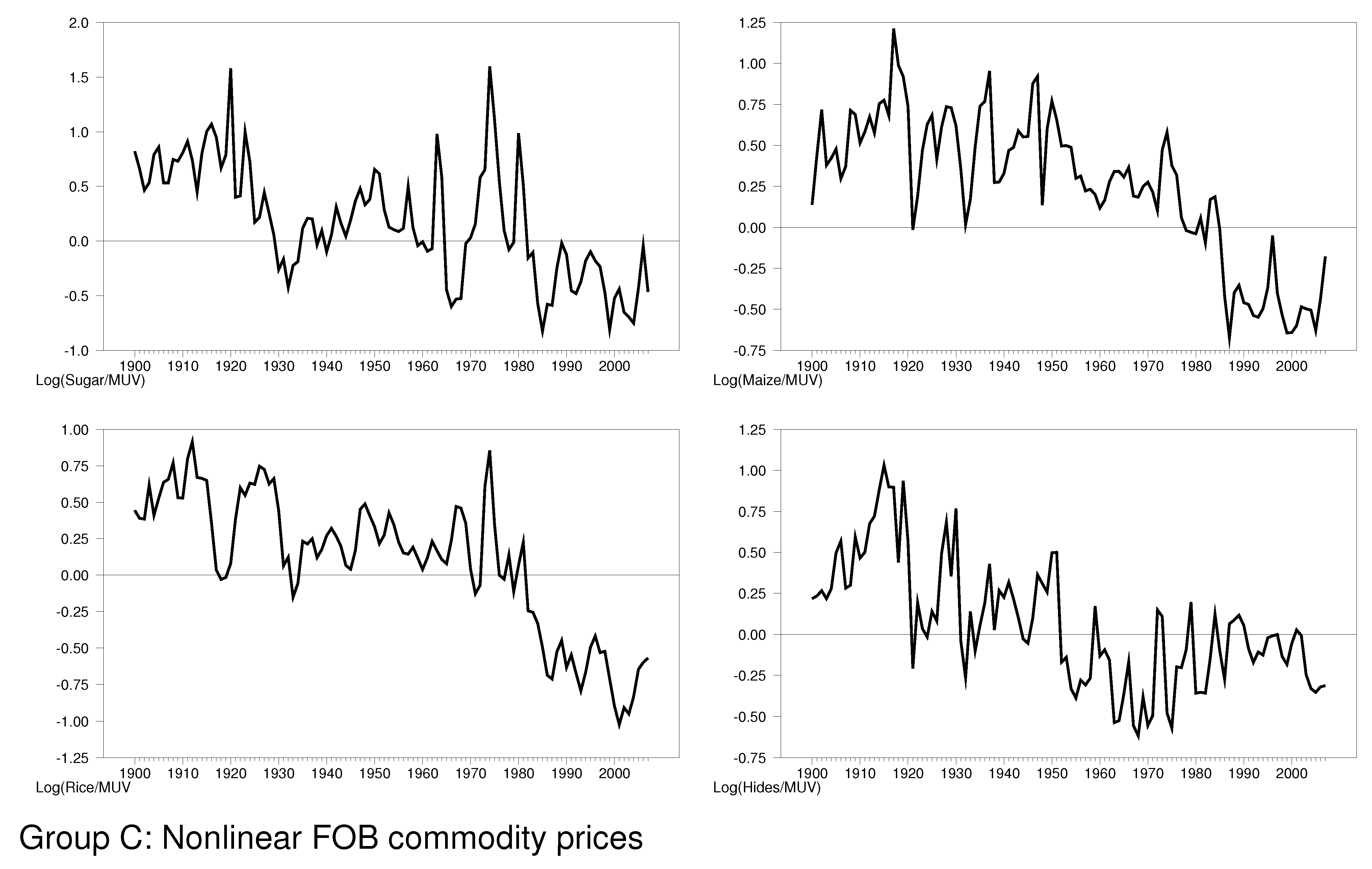
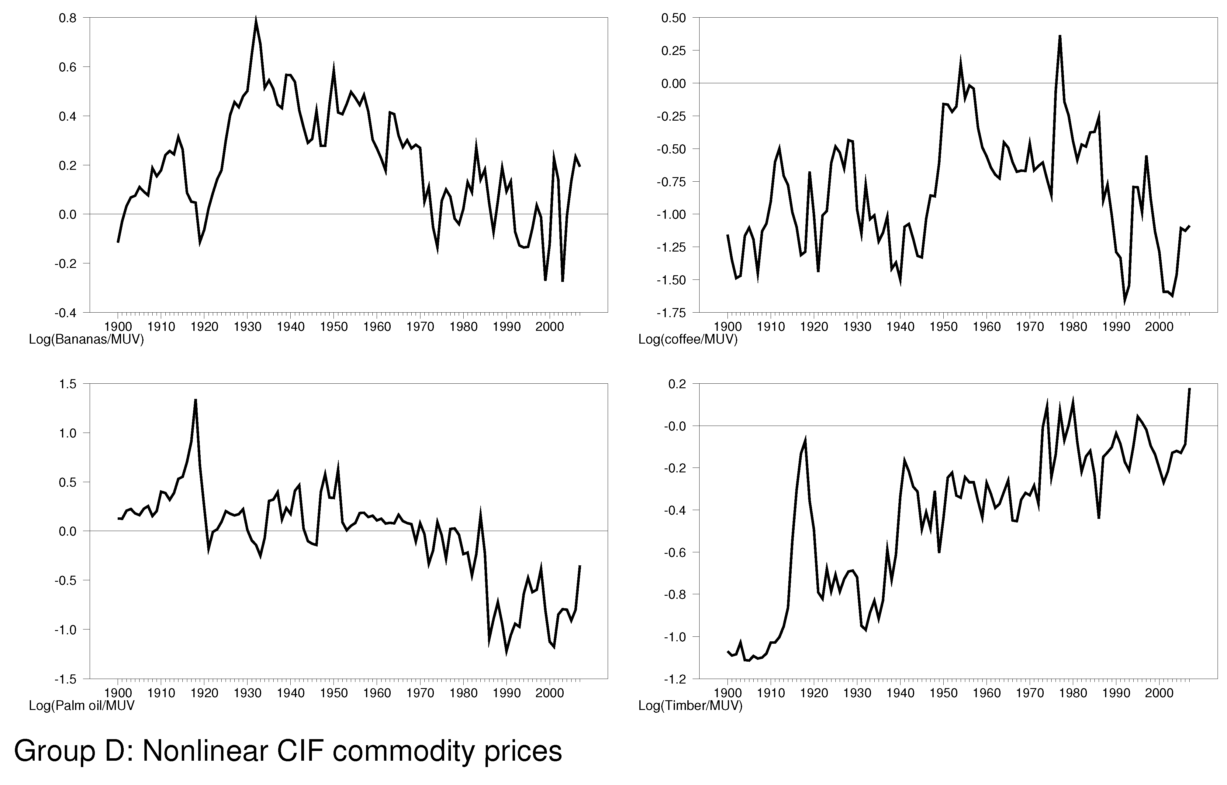
This paper uses the extended version of the Grilli and Yang (1988) data set, which is developed by Pfaffenzeller et al. (2007). The updated data set extends the annual original index and its 24 compositions to 2007. Table 1 gives a brief description of the origin, destination, terms of trade, i.e., border price, and the nonlinear model classification suggested by Fahmy (2011, 2014, 2017). Group A is the ARCH group for storable commodities. This group consists of 8 commodities: tobacco, cotton, jute, lead, aluminum, tea, silver, and wool. Group B is the linear group. This group also consists of 8 commodities: tin, lamb, zinc, rubber, copper, cocoa, wheat, and beef. Group C is the nonlinear FOB group. This group includes four commodities: sugar, rice, maize, and hides. Finally, group D is the nonlinear CIF group. It includes bananas, palm oil, coffee, and timber. We will follow the previous four classifications in the present analysis to justify the results. In particular, we will use the nonlinearity (model type) or term of trade (price type) suggested by these classifications to provide a rationale for accepting or rejecting the PS hypothesis. The data generating process is defined as , where is an index of manufactured goods’ unit values, when an aggregate analysis is conducted, or i is the price of an individual primary commodity when an individual analysis is carried out. Figure 1 shows the data generating process for the logarithm of the real index. Figure 2, Figure 3, Figure 4 and Figure 5 show plots of the logarithms of the individual real commodity prices in Group A, B, C, and D, respectively.
3.2. Wavelets Analysis
The rationale behind using wavelets analysis rests on the fact that certain economic relationships behave differently over different time scales such that the conventional analysis is not adequate to separating and revealing the time scale relationships between the variables under investigations. Wavelets analysis has this appealing feature of separating a time series into time and scale components; therefore, instead of considering the net relationship over all time scales, one can consider a set of relationships, one for each time scale.
This paper uses a wavelet transform to study the relationship between the prices of primary goods and manufactured goods in the updated Grilli and Yang (1988) data set over different time scales. The main aim is to investigate whether the hypothesis of a secular decline in the relative price of primary commodities is supported by the data or not.
A wavelet transform is a tool that dissects data or functions into different frequency components, and then studies each component with a resolution matched to its scale (Daubechies 1992). The wavelet decomposition in this paper is made with respect to the so-called symmlets basis and is done through the discrete wavelet transform (DWT) methodology.2
The DWT methodology can be presented briefly as follows. Let be a data generating process, e.g., T observations pertaining to a real valued time series. Assume that T is an integer multiple of where M is a positive integer. The discrete wavelet transform of level J is an orthonormal transform of defined by
where is an orthonormal real-valued matrix, i.e., so and are real valued vectors of wavelet coefficients at scale j and location The real valued vector is made up of scaling coefficients. Thus, the first elements of are wavelet coefficients and the last elements are scaling coefficients, where Suppose, for instance, that the vector contains 256 observations so that For the DWT consists of 6 real-valued vectors of wavelets coefficients such that the length of and one vector of scale coefficients of order as
or more explicitly
The multiresolution analysis of the data leads to a better understanding of wavelets. The idea behind multiresolution analysis is to express as the sum of several new series, each of which is related to variations in at a certain scale. Since the matrix is orthonormal, we can express as and partition the columns of commensurate with the partitioning of to obtain
where is a matrix, and is a matrix. Thus, the multiresolution analysis of a series can be defined by expressing as a sum of several new series, each of which is related to variations in at a certain scale; that is,
Equation (11) expresses the decomposition of the data generating process into orthogonal series components (details) and (smooth) at different scales.3
4. Empirical Analysis
We apply the DWT decomposition in Equation (11) to , for every commodity price i in the data set, and . The multiresolution analysis decomposes the 108 annual observations (1900–2007) available on the time series into four details; , and one smooth components The time scale stands for the finest level in the series and represents the highest frequency that occurs at the 2-year scale, stands for the next finest level in the series and represents the 4-year scale, for the 8-years scale, and for the 16-year scale. Finally, represents the long run trend in the series. Thus, captures the short run behavior of the time series, whereas captures the long run. The next step is to run the regression in Equation (6), for each commodity price i, twice, one time for short run time scale, , and another for the long run trend, Finally, we test the restriction that in the short- and the long-run.
Table 2 summarizes the previous results for the commodity index, i.e., for in In particular, the table shows the ordinary least squares estimates of the slope coefficient, , in the decomposition of Equation (6) for the Grilli and Yang commodity price index, where the value between brackets underneath the coefficient is the p-value. Although, we care about the estimation results pertaining to (short run) and (long run), for the sake of completeness, we report the results for all resolutions. The null hypothesis is not rejected in the short run and in the long run. Moreover, we also note that the null hypothesis is not rejected in the short run and long run. Thus, the results do not support the PS hypothesis for the real Grilli and Yang commodity price index. This result is consistent with the findings of Von Hagen (1989), who uses the same co-integration approach. It is also consistent with other studies that do not support the PS hypothesis, e.g., Powell (1991).
We repeat the same analysis for each individual real commodity price series and report the results in Table 3. By looking at the results in Table 3 and following Fahmy’s (2011, 2014, 2017) classification of commodity prices, we note that the PS hypothesis is not supported in the long run for all storable ARCH commodity prices (Group A), with the exception of wool. One explanation is that most of these real commodity prices are settlement and auction prices that are more likely to display ARCH pattern in their volatility rather than a downward trend. The PS hypothesis is also not supported in the long run for all linear commodity prices (Group B), with the exception of beef. It seems, however, that most of the linear group series support the PS hypothesis in the short run. This could be justified by the early structural breaks in the series in 1921 (Cuddington and Urzua 1989) and the breaks in 1937 and 1975 (Powell 1991).
Before discussing the results pertaining to border prices, i.e., Groups C and D, it is worth noting that the real prices of all commodities in these two groups were considered in Fahmy (2011). The author, as a starting point of the analysis, tests for stationarity and does not reject the stationarity in the price series. He further considers the hypothesis that they might be nonlinear. The author then proceeds to test the linearity hypothesis in for every i price against the smooth transition regression model with a set of potential transition/regime-driving variables that includes oil price, inflation, a time trend, and the autoregressive lags of The author reports that, for FOB prices, the real price of sugar, rice, and maize are nonlinear and driven by their autoregressive lags, whereas the nonlinearity in hides is driven by inflation.4 On the other hand, for CIF prices, the author documents that the price of oil is the best exogenous transition variable that can capture the nonlinearity of CIF prices. Guided by Fahmy’s (2011) results and the present PS tests results for hides, bananas, palm oil, coffee, and timber in Table 3, it seems that the PS hypothesis is not supported for all nonlinear real border prices (FOB or CIF) that are driven by exogenous transition variables (e.g., inflation and oil price). This is sensible because if the price series is nonlinear and stationary, the resulting mean reversion behavior should contradict the PS hypothesis. This finding supports the argument that classifying commodity prices according to their border prices contribute to the assessment of the PS hypothesis (RQ2).
The puzzling result, however, is the support of the PS hypothesis for stationary nonlinear FOB series that are driven by their autoregressive lags as shown from the PS tests results for sugar, rice, and maize in Table 3. One reasonable explanation for this anomaly is that when nonlinearity in a time series is driven by one of its autoregressive lags , for , the multiresolution analysis smooths the series over various time scales, thus amplifying the effect of structural breaks. This, in turn, could lead to a rejection of in some time scales and an acceptance in others. For instance, the PS hypothesis for all three commodities (sugar, rice, and maize) is not supported in the intermediate time scales (4-year and 8-year scales) as shown from the estimation results in the third and fourth columns of Table 3. The implication of this finding is that the choice of the econometric model and the existence of structural breaks do impact the PS hypothesis. This is consistent with the consensus in the empirical literature that the assessment of the PS depends on the starting point of the analysis (e.g., Ardeni and Wright 1992; Bleaney and Greenaway 1993; Cuddington and Urzua 1989; Grilli and Yang 1988; Harvey et al. 2010; Helg 1991; Kellard and Wohar 2006; Leon and Soto 1997; Lutz 1999; Newbold and Vougas 1996; Powell 1991; Sapsford 1985; Spraos 1980; Thirlwall and Bergevin 1985; Trivedi 1995; Zanias 2005) While the focus of the present study is to test the PS in the short- and long-run, i.e., in the 2-year and 16-year scale, respectively, it is worth noting that the impact of structural breaks when a different econometric model is used over the entire period of the price series is crucial on the assessment of the PS hypothesis. Ocampo and Parra (2004) argue that deteriorations in the terms of trade have been discontinuous aside from the 1920s and the 1980s periods. Balagtas and Holt (2009) add that standard unit root tests, such as Perron’s (1989) test, may provide misleading results price depending on the extent of structural breaks in the data. For that reason, recent research examining the PS hypothesis has focused on employing unit root tests where the possibility of structural breaks is allowed (e.g., Cuddington et al. 2006; Kellard and Wohar 2006; Leon and Soto 1997; Zanias 2005).
5. Conclusions
In this paper, we use a recent update of the Grilli and Yang (1988) data set on primary commodity prices to investigate the PS hypothesis. We employ wavelets analysis to the logarithm of the real Grilli and Yang commodity price index and to the individual commodities forming it. We use a discrete wavelet transform to decompose the time series into different time scales. We then fit Von Hagen’s (1989) co-integration framework to the short-term (2-year scale) and long-term (16-year scale) of the decomposed series to test the PS hypothesis.
The results do not support the PS hypothesis in the aggregate real Grilli and Yang commodity price index. As for the individual commodities forming it, the PS hypothesis is not supported for the majority of the primary commodity prices in the long run. As shown from the last column of Table 3, the PS hypothesis is supported for only 5 commodity prices (wool, beef, rice, maize, and timber) out of 24 commodities in total. In the short run, however, the hypothesis is supported for the majority of the commodities (16 out of 24).
In addition to the technical properties of the price series, e.g., stationarity, nonlinearity, and the existence of structural breaks, we show that border price classification is a key factor in the assessment of the PS hypothesis. Nonlinear FOB and CIF real commodity prices that are driven by exogenous regime-driving macroeconomic variables (e.g., inflation and oil price) are unlikely to display downward trends because the fluctuations in the exogenous regime-driving variables impact their nonlinear behavior. Thus, the PS hypothesis is unlikely to be supported for this type of border prices. Our results confirm the previous rationale; the PS hypothesis is not supported for all FOB and CIF prices in the Grilli and Yang commodity prices that are driven by exogenous transition variables. This justification is of particular importance to international trade regulators and policymakers of developing economies that depend mainly on primary commodities in their exports. The results also improve our understanding of the behavior of nonlinear real border prices.
While considerable progress has been made in examining the PS hypothesis, there is room for additional work on this topic. A particular potential fruitful area for future research is examining the PS hypothesis in different classifications of commodity prices. This paper focuses on the terms of trade classification. However, studying the impact of other potential classifications or commodity aggregations on the PS hypothesis is warranted. For instance, it would be interesting to examine the impact of the level of aggregation of primary products categories, i.e., the commodity heterogeneity of the sectors considered, that are considered in Fanelli and Giglio (2020) on the PS hypothesis. Another interesting factor is the impact of the changes in the quality of manufactured goods. Long-term changes in the terms of trade between primary products and manufacturers are sensitive to the treatment of quality change Lipsey (1994). Thus, a re-examination of the PS hypothesis that accounts for quality change among other factors is an issue worth investigating.
Funding
This research received no external funding.
Institutional Review Board Statement
Not applicable.
Informed Consent Statement
Not applicable.
Data Availability Statement
Data sharing not applicable.
Conflicts of Interest
The author declares no conflict of interest.
| 1. | The is a trade-weighted index of the five major developed countries’ (France, Germany, Japan, United Kingdom, and United States) exports of manufactured commodities to developing countries. |
| 2. | For an excellent reference, see Percival and Walden (2000). |
| 3. | Because the terms at different scales represent components of y at different resolutions, the approximation is called multiresolution decomposition. |
| 4. |
References
- Ardeni, Pier Giorgio, and Brian Wright. 1992. The Prebisch-Singer hypothesis: A reappraisal independent of stationarity hypothesis. Economic Journal 102: 803–12. [Google Scholar] [CrossRef]
- Beck, Stacie. 2001. Autoregressive conditional heteroskedasticity in commodity spot prices. Journal of Applied Econometrics 16: 115–32. [Google Scholar] [CrossRef]
- Balagtas, Joseph V., and Matthew T. Holt. 2009. The commodity terms of trade, unit roots, and nonlinear alternatives: A smooth transition approach. American Journal of Agricultural Economics 91: 87–105. [Google Scholar] [CrossRef] [Green Version]
- Bleaney, Michael, and David Greenaway. 1993. Long-run trends in the relative price of primary commodities and in the terms of trade of developing countries. Oxford Economic Papers 45: 349–63. [Google Scholar] [CrossRef]
- Box, George E. P., and Gwilym M. Jenkins. 1970. Time Series Analysis, Forecasting and Control. San Francisco: Holden Day. [Google Scholar]
- Cuddington, John T., Rodney Ludema, and Shamila A. Jayasuriya. 2006. Prebisch-Singer Redux. In Natural Resources: Neither Curse Nor Destiny. Edited by Daniel Lederman and William F. Maloney. Stanford: Stanford University Press, pp. 103–40. [Google Scholar]
- Cuddington, John T., and Carlos M. Urzua. 1989. Trends and cycles in the net barter terms of trade: A new approach. Economic Journal 99: 426–42. [Google Scholar] [CrossRef]
- Daubechies, Ingrid. 1992. Ten Lectures on Wavelets. Philadelphia: Society for Industrial and Applied Mathematics. [Google Scholar]
- Deaton, Angus. 1999. Commodity prices and growth in Africa. Journal of Economic Perspectives 13: 23–40. [Google Scholar] [CrossRef] [Green Version]
- Dickey, David A., and Wayne A. Fuller. 1979. Distributions of the estimators for autoregressive time series with a unit root. Journal of The American Statistical Association 74: 427–31. [Google Scholar]
- Engle, Robert F., and Clive W. J. Granger. 1987. Co-integration and error correction: Representation, estimation, and testing. Econometrica 55: 251–76. [Google Scholar] [CrossRef]
- Fahmy, Hany. 2011. Regime Switching in Commodity Prices. Ph.D. dissertation, Concordia University, Montreal, QC, Canada. [Google Scholar]
- Fahmy, Hany. 2014. Modelling nonlinearity in commodity prices using smooth transition regression models with exogenous transition variables. Statistical Methods and Applications 23: 577–600. [Google Scholar] [CrossRef]
- Fahmy, Hany. 2017. Classifying and modelling nonlinearity in commodity prices using Incoterms. The Journal of International Trade and Economic Development 9: 169–84. [Google Scholar]
- Fanelli, Rosa Maria, and Alessandro Giglio. 2020. The ‘similarity’ of agri-food trade flows between the EU-28 and the Asia-50. The International Trade Journal. [Google Scholar] [CrossRef]
- Granger, Clive W. J., and Timo Teräsvirta. 1993. Modelling Nonlinear Economic Relationships. Oxford: Oxford University Press. [Google Scholar]
- Grilli, Enzo R., and Maw Cheng Yang. 1988. Primary commodity prices, manufactured goods prices, and the terms of trade of developing countries: What the long run shows. World Bank Economic Review 2: 1–47. [Google Scholar] [CrossRef]
- Gustafson, Robert L. 1958. Carryover Levels for Grains. U.S.D.A. Technical Bulletin No. 1178. Washington, DC: U.S.D.A. [Google Scholar]
- Harvey, David I., Neil M. Kellard, Jakob B. Madsen, and Mark E. Wohar. 2010. The Prebisch-Singer hypothesis: Four centuries of evidence. The Review of Economics and Statistics 92: 367–77. [Google Scholar] [CrossRef]
- Helg, Rodolfo. 1991. A note on the stationarity of the primary commodities relative price index. Economics Letters 36: 55–60. [Google Scholar] [CrossRef]
- Kellard, Neil, and Mark E. Wohar. 2006. On the prevalence of trends in commodity prices. Journal of Development Economics 79: 146–67. [Google Scholar] [CrossRef]
- Leon, Javier, and Raimundo Soto. 1997. Structural breaks and long-run trends in commodity prices. Journal of International Development 3: 44–57. [Google Scholar] [CrossRef]
- Lewis, William Arthur. 1954. Economic development with unlimited supplies of labour. Manchester School of Economics and Social Studies 22: 139–91. [Google Scholar] [CrossRef]
- Lipsey, Robert E. 1994. Quality Change and Other Influences on Measures of Export Prices of Manufactured Goods and the Terms of Trade between Primary Products and Manufacturers. Working Paper No. 4671. Cambridge: NBER—National Bureau of Economic Research. [Google Scholar]
- Luukkonen, Ritva, Pentti Saikkonen, and Timo Teräsvirta. 1988. Testing linearity against smooth transition autoregressive models. Biometrika 75: 491–9. [Google Scholar] [CrossRef]
- Lutz, Matthias G. 1999. A general test of the Prebisch-Singer hypothesis. Review of Development Economics 3: 44–57. [Google Scholar] [CrossRef]
- Muth, John F. 1961. Rational expectations and the theory of price movements. Econometrica 29: 315–35. [Google Scholar] [CrossRef]
- Newbold, Paul, and Dimitrios Vougas. 1996. Drift in the relative prices of primary commodity prices: A case where we care about unit roots. Applied Economics 28: 653–61. [Google Scholar] [CrossRef]
- Ocampo, José Antonio, and María Ángela Parra. 2004. The terms of trade for commodities in the twentieth century. In Econ Working Paper Archive. International Trade Series No. 0402006; Santiago: CEPAL. [Google Scholar]
- Percival, Donald B., and Andrew T. Walden. 2000. Wavelet Methods for Time Series Analysis. Cambridge: Cambridge University Press. [Google Scholar]
- Perron, Pierre. 1989. The great crash, the oil price shock and the unit root hypothesis. Econometrica 57: 1361–401. [Google Scholar] [CrossRef]
- Persson, Anna, and Timo Teräsvirta. 2003. The net barter terms of trade: A smooth transition approach. International Journal of Finance and Economics 8: 81–97. [Google Scholar] [CrossRef]
- Pfaffenzeller, Stephan, Paul Newbold, and Anthony Rayner. 2007. A short note on updating the Grilli-Yang commodity price index. World Bank Economic Review 21: 151–63. [Google Scholar] [CrossRef]
- Phillips, Peter C. B., and Peter Schmidt. 1989. Testing for a Unit Root in the Presence of Deterministic Trends. Cowels Foundation Discussion Papers 933. New Haven: Cowels Foundation, Yale University. [Google Scholar]
- Powell, Andrew. 1991. Commodity and developing country terms of trade: What does the long run show? Economic Journal 101: 1485–96. [Google Scholar] [CrossRef]
- Prebisch, Raul. 1950. The economic development of Latin America and its principal problems. Economic Bulletin For Latin America 7: 1–12. [Google Scholar]
- Sapsford, David. 1985. The statistical debate on the net barter terms of trade between primary commodities and manufacturers: A comment and some additional evidence. Economic Journal 95: 781–88. [Google Scholar] [CrossRef]
- Singer, Hans W. 1950. The distributions of gains between investing and borrowing countries. American Economic Review 40: 473–85. [Google Scholar]
- Spraos, John. 1980. The statistical debate on the net barter terms of trade between primary commodities and manufacturers. Economic Journal 90: 107–28. [Google Scholar] [CrossRef]
- Teräsvirta, Timo. 1994. Specification, estimation, and evaluation of smooth transition autoregressive models. Journal of American Statistical Association 89: 208–18. [Google Scholar]
- Thirlwall, Anthony P., and James Bergevin. 1985. Trends, cycles, and asymmetries in the terms of trade of primary commodities from developed and less developed countries. World Development 13: 805–17. [Google Scholar] [CrossRef]
- Trivedi, Pravin K. 1995. Tests of some hypotheses about the time series behavior of commodity process. In Advances in Econometrics and Quantitative Economics. Edited by G. S. Maddala, T. N. Srinivasan and Peter C. B. Phillips. Oxford: Blackwell, pp. 382–412. [Google Scholar]
- Von Hagen, Juergen. 1989. Relative commodity prices and cointegration. Journal of Business & Economic Statistics 74: 497–503. [Google Scholar]
- Zanias, George P. 2005. Testing for trends in the terms of trade between primary commodities and manufactured goods. Journal of Development Economics 78: 49–59. [Google Scholar] [CrossRef]
Figure 1.
A plot of the logarithm of the annual real Grilli and Yang commodity price index from 1900 to 2007.
Figure 1.
A plot of the logarithm of the annual real Grilli and Yang commodity price index from 1900 to 2007.

Figure 2.
A plot of for every commodity price i in Group A in Table 1.
Figure 2.
A plot of for every commodity price i in Group A in Table 1.

Figure 3.
A plot of for every commodity price i in Group B in Table 1.
Figure 3.
A plot of for every commodity price i in Group B in Table 1.

Figure 4.
A plot of for every commodity price i in Group C in Table 1.
Figure 4.
A plot of for every commodity price i in Group C in Table 1.

Figure 5.
A plot of for every commodity price i in Group D in Table 1.
Figure 5.
A plot of for every commodity price i in Group D in Table 1.


Table 1.
Trading route, border price, top importer and exporter, and Fahmy’s (2011, 2017) work suggested classification for each individual commodity in the Grilli and Yang data set.
| Series | Origin | Destination | Price | Top Exporter | Top Importer | Classification; Model |
|---|---|---|---|---|---|---|
| Tobacco | NA | USA | CIF | Brazil/USA | Russia/USA | A; ARCH |
| Cotton | Memphis | Europe | CIF | USA | China | A; ARCH |
| Jute | Bangladesh | NA | FOB | India | Various | A; ARCH |
| Lead | London Metal Exchange | Settlement | A; ARCH | |||
| Aluminum | London Metal Exchange | Settlement | A; ARCH | |||
| Tea | NA | Auction | A; ARCH | |||
| Silver | Handy & Harry | A; ARCH | ||||
| Wool | Australia Exchange | Spot quote | A; ARCH | |||
| Tin | London Metal Exchange | Settlement | B; Linear | |||
| Lamb | New Zealand | London | Wholesale | New Zealand | UK | B; Linear |
| Zinc | London Metal Exchange | Settlement | B; Linear | |||
| Rubber | Rubber Traders Association | Spot Price | B; Linear | |||
| Copper | London Metal Exchange | Settlement | B; Linear | |||
| Cocoa | London and US Exchange | Option Price | B; Linear | |||
| Wheat | Canada | NA | FOB | USA | China/Japan | B; Linear |
| Beef | Argentina | NA | FOB | Australia | USA | B; Linear |
| Sugar | Caribbean Ports | Various | FOB | Brazil | Russia | C; nonlinear FOB |
| Rice | Bangkok | NA | FOB | Thailand | Philippines | C; nonlinear FOB |
| Maize | Gulf Port | NA | FOB | USA | Japan | C; nonlinear FOB |
| Hides | USA | NA | FOB | C; nonlinear FOB | ||
| Bananas | NA † | Gulf ports | CIF | India / Brazil | USA | D; nonlinear CIF |
| Palm oil | Malaysia | Netherlands | CIF | Malaysia | Netherlands | D; nonlinear CIF |
| Coffee | Average ‡ | New York | CIF | Brazil | US/Germany | D; nonlinear CIF |
| Timber | NA † | UK | CIF | NA | NA | D; nonlinear CIF |
†: Not available. ‡: The price is arithmetic average of El Salvador, Guatemala, and Mexico.
Table 2.
Multiresolution decomposition of logarithm of the real Grilli and Yang commodity price index. The reported values are the least squares estimates of the slope coefficient in Equation (6). The p-values are reported in brackets underneath the coefficients.
Table 2.
Multiresolution decomposition of logarithm of the real Grilli and Yang commodity price index. The reported values are the least squares estimates of the slope coefficient in Equation (6). The p-values are reported in brackets underneath the coefficients.
| Equation (6): | ||||
|---|---|---|---|---|
| Resolution | Scale | Decision criterion | ||
| SR; 2-year | Accept | |||
| 4-year | ||||
| 8-year | ||||
| 16-year | ||||
| LR trend | Accept | |||
Table 3.
Multiresolution decomposition of logarithm of real individual commodity prices in the Grilli and Yang data set. The reported values are the least squares estimates of the slope coefficients in Equation (6). The p-values are reported in brackets underneath the coefficients. DF denotes the degrees of freedom.
| Time Scale | SR | 4-Year | 8-Year | 16-Year | LR | ||
|---|---|---|---|---|---|---|---|
| Crystals | D | D | D | D | S | SR | LR |
| Group A: ARCH commodity prices | |||||||
| Tobacco | Reject | Accept | |||||
| Cotton | Reject | Accept | |||||
| Jute | Reject | Accept | |||||
| Lead | Reject | Accept | |||||
| Aluminum | Reject | Accept | |||||
| Tea | Reject | Accept | |||||
| Silver | Reject | Accept | |||||
| Wool | Accept | Reject | |||||
| Group B: Linear AR commodity prices | |||||||
| Tin | Reject | Accept | |||||
| Lamb | Reject | Accept | |||||
| Zinc | Reject | Accept | |||||
| Rubber | Reject | Accept | |||||
| Copper | Accept | Accept | |||||
| Cocoa | Accept | Accept | |||||
| Wheat | Accept | Accept | |||||
| Beef | Reject | Reject | |||||
| Group C: Free on Board (FOB) commodity prices | |||||||
| Sugar | Reject | Reject | |||||
| Rice | Reject | Reject | |||||
| Crystals | D | D | D | D | S | SR | LR |
| Group C: Free on Board (FOB) commodity prices | |||||||
| Maize | Reject | Reject | |||||
| Hides | Accept | Accept | |||||
| Group D: Cost Insurance and Freight (CIF) commodity prices | |||||||
| Bananas | Accept | Accept | |||||
| Palm oil | Accept | Accept | |||||
| Coffee | Accept | Accept | |||||
| Timber | Reject | Reject | |||||
Publisher’s Note: MDPI stays neutral with regard to jurisdictional claims in published maps and institutional affiliations. |
© 2021 by the author. Licensee MDPI, Basel, Switzerland. This article is an open access article distributed under the terms and conditions of the Creative Commons Attribution (CC BY) license (https://creativecommons.org/licenses/by/4.0/).
Share and Cite
MDPI and ACS Style
Fahmy, H. A Reappraisal of the Prebisch-Singer Hypothesis Using Wavelets Analysis. J. Risk Financial Manag. 2021, 14, 319. https://doi.org/10.3390/jrfm14070319
AMA Style
Fahmy H. A Reappraisal of the Prebisch-Singer Hypothesis Using Wavelets Analysis. Journal of Risk and Financial Management. 2021; 14(7):319. https://doi.org/10.3390/jrfm14070319
Chicago/Turabian StyleFahmy, Hany. 2021. "A Reappraisal of the Prebisch-Singer Hypothesis Using Wavelets Analysis" Journal of Risk and Financial Management 14, no. 7: 319. https://doi.org/10.3390/jrfm14070319