Article

Modeling Market Order Arrivals on the German Intraday Electricity Market with the Hawkes Process

by
Nikolaus Graf von Luckner
1,* and
Rüdiger Kiesel
2
1
be.storaged GmbH, Fritz-Bock-Straße 5, GER-26121 Oldenburg, Germany
2
Chair for Energy Trading and Finance, University of Duisburg-Essen, Universitätsstraße 2, GER-45141 Essen, Germany
*
Author to whom correspondence should be addressed.
J. Risk Financial Manag. 2021, 14(4), 161; https://doi.org/10.3390/jrfm14040161
Submission received: 17 March 2021 / Revised: 1 April 2021 / Accepted: 2 April 2021 / Published: 5 April 2021

Abstract

:
We use point processes to analyze market order arrivals on the intraday market for hourly electricity deliveries in Germany in the second quarter of 2015. As we distinguish between buys and sells, we work in a multivariate setting. We model the arrivals with a Hawkes process whose baseline intensity comprises either only an exponentially increasing component or a constant in addition to the exponentially increasing component, and whose excitation decays exponentially. Our goodness-of-fit tests indicate that the models where the intensity of each market order type is excited at least by events of the same type are the most promising ones. Based on the Akaike information criterion, the model without a constant in the baseline intensity and only self-excitation is selected in almost 50% of the cases on both market sides. The typical jump size of intensities in case of the arrival of a market order of the same type is quite large, yet rather short lived. Diurnal patterns in the parameters of the baseline intensity and the branching ratio of self-excitation are observable. Contemporaneous relationships between different parameters such as the jump size and decay rate of self and cross-excitation are found.

1. Introduction

On the spot market for power deliveries in Germany (operated by EPEX SPOT SE), contracts with hourly delivery are traded in an auction with gate closure at 12 noon on the day before the delivery day. This is followed by continuous trading from 3 pm on the day before the delivery day until half an hour before delivery start (5 min before delivery start in the area of the local transmission system operator). The latter market is typically referred to as intraday market (IDM). Participants on the IDM may choose between placing limit orders (LOs), which are collected in the limit order book (LOB), and market orders (MOs), which execute one or more LOs from the LOB partially or entirely. More details on the organization of the IDM may be found in EPEX SPOT SE (2020).
On markets with continuous trading, events such as the placement of a buy MO occur randomly in time. They may be modeled with point processes for which the homogeneous Poisson process is the most basic example. Point processes are characterized by their intensity function, which is linked to the probability of an event occurring. The intensity function of the homogeneous Poisson process is a constant. More sophisticated point processes have a time-varying and potentially stochastic intensity. The Hawkes process is a stochastic-intensity point process, which has the property that its intensity function may undergo excitation. That means the arrival of an event causes the intensity to jump change, with this jump change decaying again over time. Hence, the intensity function of the Hawkes process has two components, namely the baseline intensity which triggers arrivals not due to excitation and the excitation part. In Hawkes (1971), where the process was originally introduced, it is assumed that the jumps are positive.
The analysis of event arrivals on markets with continuous trading has been subject to research as soon as data on arrivals become available. Jain and Joh (1988) is an early work that states that the average diurnal pattern of trade volumes is U-shaped. Their findings motivated the widely-cited work of Admati and Pfleiderer (1988) in which a theoretic explanation for the concentration of transactions is provided, more specifically diurnal patterns and random clustering of transactions. In Easley and O’Hara (1992), an alternative explanation for such clustering is presented. In Biais et al. (1995), empirical evidence for random clustering of transactions is provided. The authors of that paper conjecture that such clusters may be due to market participants splitting their MOs, market participants mimicking other market participants, or market participants reacting to new information in timely proximity, see also Gould et al. (2013).
Engle and Russell (1998) present a model for the durations between consecutive transactions on a financial market, which has both diurnal patterns and random clustering of transactions incorporated. They state that the Hawkes process is not appropriate for modeling arrivals of financial transactions due to the fact that it is in real time and not in event time. This causes some transactions to have the same impact on the intensity at some point in time no matter how many transactions there have been between that transaction and the same point in time. Nevertheless, the Hawkes process made its way to being applied to event data from financial markets. Apparently, it was Bowsher (2007) who first used a bivariate Hawkes process to model the times of transactions and mid price changes.
Following Bowsher, the Hawkes process has been frequently used in the context of modeling events on markets with continuous trading. Bacry et al. (2015) and Hawkes (2018) provide overviews of research on the Hawkes process in finance and market microstructure in particular. In Bacry and Muzy (2014), for example, market order arrivals and changes of market prices are modeled with the Hawkes process. Da Fonseca and Zaatour (2014) provide explicit formulas for the moments of the intensity of a particular Hawkes process and the number of arrivals over time. Yet another interesting example is Rambaldi et al. (2017), where the process of orders arriving on a futures market is divided into subprocesses depending on order size.
It is not that the Hawkes process is only used in the context of continuous trading. In Errais et al. (2010), for example, it is used to model corporate defaults. Eyjolfsson and Tjøstheim (2018) is an example where the Hawkes process is used in the context of electricity price modeling.
A paper of particular importance for this work is Chen and Hall (2013) where the authors use a Hawkes process with time-varying baseline intensity to model transaction arrivals for some stock. Time dependence of the rate at which transactions on the IDM occur is also observable, see Scharff and Amelin (2016), Narajewski and Ziel (2019), and Kremer et al. (2020). Favetto (2020) and Kramer and Kiesel (2021) are works on modeling market order arrivals on the IDM with the Hawkes process, which also departed from analysis in Section 2.
One contribution of this work is empirical evidence for higher intensity of MO arrivals close to gate closure and clustering in MO arrivals. Building on these observations, we address the question whether the Hawkes process is suited to model the clustering. We leave the question whether other models that result in clustering of MO arrivals may also be suited to future research. The same holds true for the assessment whether one clustering model outperforms another. The goodness-of-fit of the Hawkes process turns out to be clearly better compared to the same model without excitation. On that basis, we identify some characteristics of the estimated Hawkes processes for each contract. Examples are a strong but short-lived self-excitation, more offspring due to MOs on the same market side than on the other market side, and a strongly negative relationship between the time-zero level of the exponential growth component of the baseline intensity and its growth rate.
The remainder of this article is organized as follows: In Section 2, we provide empirical analyses that are aimed at informing on the time dependence of the baseline intensity and the prevalence of clustering. Then we introduce the multivariate Hawkes process and outline how we estimate the parameters, assess goodness-of-fit, and compare models with different assumptions regarding the dependence structure between different event types with each other, see Section 3. The results are provided in Section 4. Furthermore, we analyze the estimated parameters in that section. Section 5 concludes with a summary and discussion of our results.

2. Empirical Analysis

We used data obtained from EPEX SPOT SE. It comprises all LOs and MOs for hourly contracts with delivery start in the second quarter of 2015 (also referred to as “Q2/2015”) which had Germany as the delivery area. All orders with delivery areas other than Germany that also appeared in the LOB for deliveries in Germany are missing. That means LOs with Germany as the delivery area that were executed by MOs with other delivery areas are contained in the data. However, LOs with delivery areas other than Germany that were executed by MOs with Germany as the delivery area are not contained.
We limited our empirical analyses to buy and sell MOs. In regards to the buy side, we consider the time at which sell LOs executed by a buy MO were removed from the LOB to be the timestamp of that MO. On the sell side, it is the time at which buy LOs executed by a sell MO were removed from the LOB. The time at which an executed LO is removed from the LOB is usually around 10 milliseconds after the time of arrival of the MO. We consider all MOs for contracts with delivery start at the same full hour of the day together, not just those for the same contract, even though our results in Section 4.1 imply that considering the MOs for each contract individually is more promising. The reason is that the number of MOs per contract is typically too small for our empirical analyses to be meaningful. We are convinced that the results of our empirical analyses are also informative with regards to the per-contract consideration.
Let us first consider frequencies of arrival times together with durations between those arrival times and the subsequent arrival times of buy and sell MOs. Given some point in time and some duration which is less than or equal to the duration between the point in time under consideration and the end of trading, this analysis provides information on how likely it is to observe an event at that point in time and how likely it is that the duration under consideration is the duration until the next event arrival. These probabilities allow conclusions to be drawn about the process that generated the arrivals. The homogeneous Poisson process is an example of such a process. In that case the probability of an event arrival at some point in time is always the same, just as the probability that some duration is the duration until the next event arrival.
In concrete terms, we determine for each buy (sell) MO how long it took for the next buy (sell) MO to arrive. Then we plot two-dimensional histograms with arrival times of buy (sell) MOs on the horizontal axis and interarrival durations on the vertical axis. Figure 1 shows the results for the buy and sell side. The upper triangle of the plot is shaded because these timestamp-duration pairs are not reachable. The plots reveal that more MOs are placed close to gate closure than after market opening, also causing the interarrival times to decrease as gate closure approaches. The simulation study in Appendix A illustrates that neither the simulated arrivals of a homogeneous Poisson process nor those of a Hawkes process as defined in Section 3.1 with constant baseline intensity result in comparable patterns. Instead, the simulated arrivals of a non-homogeneous Poisson process with increasing intensity close to gate closure as well as those of a Hawkes process with increasing baseline intensities close to gate closure result in similar patterns. One may also observe that in the hours after market opening durations in the region of the maximum durations occur only rarely. This indicates that in the hours before gate closure, the baseline intensities reach levels that are high enough to make the incident of no event very unlikely. The simulation study in Appendix A also illustrates this connection. Hence, a suitable model for the baseline intensity should allow for a rather short time window before gate closure during which the baseline intensity is substantially higher.
Let us now analyze empirical evidence for clustering in the arrivals of buy and sell MOs that may be due to self or cross-excitation. In Hewlett (2006), an empirical analysis is provided which indicates that clustering prevails in buy and sell MO arrivals on foreign exchange markets. The analysis involves splitting the time after the arrival of each buy and sell MO into intervals of a fixed length and open on the left side, and counting the number of buy and sell MOs in these intervals. Then the mean numbers of buy and sell MO arrivals in each interval after the arrival of a buy or sell MO are computed. A decrease in the mean number of buy (sell) MO arrivals after the arrival of a buy (sell) MO with increasing lag implies that buy (sell) MOs tend to arrive in clusters, which may be due to self-excitation. A decrease in the mean numbers of buy (sell) MO arrivals after the arrival of a sell (buy) MO with increasing lag implies that buy (sell) MOs tend to arrive in clusters, which may be due to cross-excitation.
We consider all buy and sell MOs which were placed for hourly contracts with delivery start in Q2/2015. Once again, we consider the contracts with delivery during one particular hour of the day together. We analyze a period of five minutes after a buy (sell) MO and split this period into intervals of five seconds. The red lines in Figure 2 reflect the results for buy MOs and the blue lines for sell MOs. The average number of buy (sell) MO arrivals after the arrival of a buy (sell) MO is high in the first interval and initially decreases from one interval to the next at a high rate, no matter which market side or delivery hour is considered. The average number of buy (sell) MO arrivals after the arrival of a sell (buy) MO is much smaller in the first interval but also decreases visibly at the beginning. Hence, clustering prevails in MO arrivals, which may be due to self- and/or cross-excitation. As the Hawkes process allows for such excitation, we analyze whether the dynamics of MO arrivals can be captured with that process in the following section.

3. Model

3.1. Definition

By ( Ω , F , P ) we denote a probability space with P the physical probability measure which is equipped with a filtration ( F t ) t 0 that satisfies the usual conditions. The stochastic process under consideration is defined on ( Ω , F , ( F t ) t 0 , P ) .
We want to model the arrivals of MOs for a specific contract that is traded on the IDM, the trading start of which we fix as t = 0 . Referring to Daley and Vere-Jones (2003), these arrivals may be thought of as occurrences of a phenomenon at random points in time t i , i = 1 , 2 , > 0 , which may be modeled with so-called point processes. We assume that t i + 1 t i > 0 , i = 1 , 2 , , which implies that the point process under consideration is orderly. As described in Brémaud (1981), a point process has a counting process ( N t ) t 0 associated with it that reflects the number of occurrences up to and including t. The counting process N t has support over the positive half line and N 0 = 0 .
We want to distinguish between d types of MOs, meaning that the point process under consideration is multivariate. As a consequence, the associated counting process is also d-dimensional. We denote the latter by ( N t ) t 0 . Each type’s process may be referred to as a marginal process, whereas the process comprising all types is called the pooled process. The orderliness of the pooled process implies that the marginal processes are also orderly.
As pointed out in Section 2, MOs on the IDM tend to arrive in clusters. A point process by which the events arrive in clusters is the Hawkes process. Its intensity may be excited by event arrivals. The definition for the multivariate Hawkes process which we provide in the following is based on Cox and Isham (1980). Let Δ N   : = N t + h N t with h > 0 and D   : = 1 , , d . A multivariate point process with associated counting process ( N t ) t 0 is a multivariate Hawkes process if:
P Δ N j = 1 Δ N k = 0 , k D \ j F t = λ t , j h + o ( h ) , j D
P Δ N j > 1 Δ N k = 0 , k D \ j F t = o ( h ) , j D
and if ( λ t ) t 0 , a d-dimensional stochastic process, which is referred to as the conditional intensity, has the form:
λ t = μ ( t ) + 0 t ϕ t u d N u ,
where μ ( t ) : R 0 R > 0 d is referred to as the baseline intensity function and ϕ ( t ) : R > 0 R 0 d × d is referred to as the excitation function.
In order to define a specific multivariate Hawkes process, its conditional intensity has to be specified. In finance literature, cubic B-splines with fixed knots have been used to model the baseline intensity functions, see e.g., Engle and Russell (1998) or Chen and Hall (2013). They appear to be particularly useful for capturing intensity patterns like the U shape discussed in Jain and Joh (1988). We suspect a baseline intensity that comprises a constant and increases exponentially towards gate closure, and choose a model that is as sparse as possible, i.e.:
μ j ( t ) = ν j + γ j e η j t , j 1 , , d ,
where ν 0 , γ > 0 , η 0 are d-dimensional vectors. We refer to ν as the constant of the baseline intensity, to γ as the growth component at time zero or time-zero growth component of the baseline intensity, and to η as the growth rate of the baseline intensity. The time-varying baseline intensity causes the Hawkes process, which is considered here to be non-stationary.
Concerning the excitation function, a prominent example is the exponential one which we assume for all the components of ϕ ( t ) , i.e.,
ϕ j k ( t ) = α j k e β j k t , j , k 1 , , d ,
where α 0 , β > 0 are d × d -dimensional matrices. The matrix α comprises the sizes by which the conditional intensities of the different types jump up in case of an event of any of the types and is therefore referred as the jump size. The matrix β comprises the rates at which these jumps decay and is therefore referred to as the decay rate. Given the exponential form of the components of β , the half-life of a jump α j k , i.e., the amount of time it takes until half of it is decayed again, is ln 2 / β j k . The average number of events of type j triggered by an event of type k is referred to as branching ratio and may be obtained by evaluating 0 ϕ j k ( u ) d u . In case of an exponential excitation function, the branching ratio is α j k / β j k . Branching ratios larger than 1 imply that the event type responsible for excitation causes an explosion of the marginal process in the sense that N j , s N j , t = for s t > 0 . For N to be non-explosive, it does not suffice that all branching ratios are smaller than 1. Instead, component-wise division of α by β has to yield a matrix which has a spectral radius strictly smaller than 1, see Theorem 7 in Brémaud and Massoulié (1996).
It is possible to make assumptions on the components of α and β . This may be useful, for example, when the objective is to model the impact of MOs on the mid price and one has reasons to believe that they neither cause the mid price to grow nor to decline in expectation in the long run. Another example is that the intensities of all contracts with delivery during a particular hour of the day are assumed to be the same as is done in Section 2. To suppress the excitation of the intensity of event type j by event type k, α j k needs to be set to 0. The model without restrictions and those with restrictions are nested, with the former referred to as full model and the latter as restricted models.

3.2. Estimation

We estimate the model parameters by maximum likelihood. While it would be possible to estimate the parameters of all d marginal processes together, we choose not to do so, the reason being that the optimization algorithm appears to converge more often if there are less parameters to be estimated.
Let L ( j ) ( θ ( j ) ) denote the likelihood function associated with λ j , where θ ( j ) is the parameter vector. If both self- and cross-excitation are allowed, the likelihood function is a mapping of R > 0 d + 1 × R 0 d + 2 R . Following Daley and Vere-Jones (2003), we minimize the negative logarithm of L ( j ) relative to the likelihood function of the unit-rate Poisson process which is denoted by L ( 0 ) , i.e.,
ln L ( j ) L ( 0 ) = i = 1 N j , T ln λ j , t i + 0 T λ j , u 1 d u ,
where T is the time at which trading ends. As already stated in Section 3.1, we fix the time at which trading starts as t = 0 . Hence, the time at which trading ends for some contract depends on the hour of the day during which delivery takes place.
Minimization of the negative log likelihood function yields the vector of estimated parameters, which we denote by θ ^ ( j ) . We use the implementation of the sequential least squares quadratic programming (SLSQP) algorithm from the Python package scipy for minimization. The reason for that is that this algorithm allows parameter constraints, which is useful in our setting because all parameters are non-negative. Furthermore, we multiply the parameters with powers of 10 in such a way that the parameters to be estimated are of similar order of a magnitude.

3.3. Goodness-of-Fit

Let ( Λ t ) t > 0 denote the compensator of some multivariate point process with associated counting process N t and conditional intensity λ t , i.e.,
Λ t = 0 t λ u d u .
By ( N ˜ t ) t > 0 , we denote the following transformation of the counting process N t :
N ˜ t = N ( Λ t 1 ) .
According to Daley and Vere-Jones (2003), the so-called random time change theorem states that the point process with which the transformed counting process is associated is a unit-rate Poisson process. Hence, if the durations between the event times which are used to estimate the parameters of the process and which are subsequently transformed with the compensator are i.i.d. unit-rate exponentially distributed, the data may be considered to be fitting to the model associated with the compensator. In this context, Lallouache and Challet (2016) use the (two-sided) Kolmogorov–Smirnov (KS) test with null hypothesis of identical distributions and the (one-sided) excess dispersion (ED) test from Engle and Russell (1998) with null hypothesis of no excess dispersion to test for unit-rate exponential distribution, and the Ljung–Box (LB) test to test for no autocorrelation. In Bowsher (2007), the same question is addressed. However, as a multivariate Hawkes process is considered, the author remarks that in addition it is necessary to pool the transformed event times of the marginal processes and test the resulting durations for no autocorrelation. In this analysis, only those events are considered, the timestamps of which are smaller than the timestamp of the last event of the marginal process which has the youngest last event. The LB test may be used again to test durations for no autocorrelation.

3.4. Model Selection

It is possible to make assumptions on the parameters of the process under consideration, as already stated in Section 3.1. An example for such an assumption is that one of the marginal processes of a bivariate Hawkes process has only self-excitation, yielding a different dependence structure compared to a bivariate Hawkes process with self- and cross-excitation in that marginal process. Ex ante it is not clear which dependence structure should be considered when inferring about what is modeled. This is particularly true when processes with different dependence structures have acceptable goodness-of-fit. However, some analyses may require selecting a model from a set of candidate models first, e.g., when analyzing the parameters controlling self- and cross-excitation of a multivariate Hawkes process.
The procedure for model selection which we adopt here is from Burnham and Anderson (2002) and builds upon information theory. The starting point is to acknowledge that there is a true model for the point process under consideration, which is unknown. We want to know how close to the true model different approximating models are. This distance is referred to as Kullback–Leibler (KL) information. The KL information may be split into an unknown constant and the relative directed distance between the true and an approximating model. It is the latter quantity which governs differences in the distance between the true model and different approximating models. The problem with computing this quantity is that knowledge of the parameters of the approximating model is required, which is not the case. This may be handled by estimating the parameters with maximum likelihood (see Section 3.2) and considering the expected KL information, where the expectation is with respect to the parameters. An estimation of this relative expected KL information is the Akaike information criterion (AIC), which is defined as:
AIC = 2 ln L ( θ ^ ) + 2 K ,
where L ( · ) is the likelihood function, θ ^ is the vector of estimated parameters, and K is the number of parameters with potentially different values. Among the approximating models, the one with the smallest AIC is the one that is estimated to be closest to the true model.
With the AIC of each approximating model at hand, it is possible to compute each model’s AIC difference, i.e., the difference between a model’s AIC and the AIC of the model with the smallest AIC. The model with the smallest AIC (also referred to as the best model) has an AIC difference of 0 and all other models have AIC differences of at least 0. The case of equal AICs and hence more than one model with zero AIC difference is theoretically possible but does not materialize in our analyses. In case of nested models, the AIC difference of the full model is bounded above by twice the difference in number of parameters because the likelihood of the full model is at least the same as the likelihood of the restricted model. The AIC difference of the restricted model is not bounded above because the amount by which the likelihood of the full model can exceed that of the restricted model is not bounded. The magnitudes of the AIC differences of the approximating models which have an AIC greater than the smallest AIC bear information on the extent to which the models are worse than the best model. In this context, Burnham and Anderson (2002) provide as a rule of thumb that an AIC difference up to 2 means that there is still substantial support for the worse model, an AIC difference between 4 and 7 means that there is considerably less support, and an AIC difference beyond 10 means that there is essentially no support.
We avoid to compare the model selection results with those that are obtained when deploying the Bayesian information criterion (BIC), which is another popular information criterion. If the true model is among the candidates, the BIC selects that model with probability 1 as the sample size goes to infinity. At the same time, derivation of the BIC does not require the true model to be among the candidates, see p. 293 et seq. in Burnham and Anderson (2002). In that case, however, the sort of parsimony which the BIC yields is unknown. The AIC does not have this weakness because the true model is considered to be unknown anyway. While our model in Section 3.1 has features which address the empirical characteristics identified in Section 2, we are very sure that it is not the true model. A simple example in this context is that our model fails to allow for zero intensity of MO arrivals if no LOs are available on the opposite side of the LOB. That is why we only consider the AIC in model selection.

4. Results

4.1. Model Subset

We analyze arrivals of buy and sell MOs on the IDM. With regards to the baseline intensity we consider the model which comprises the constant ν and the model which does not. Concerning excitation, the first model that we consider is the one where neither the events of the same type nor the events of the other type cause excitation of each type’s conditional intensity. In such a case, the process is a non-homogeneous Poisson process (NHPP). Then we consider the models where only one of the two types causes excitation of each type’s conditional intensity. This may be either the same type (self-excitation) or the other one (cross-excitation). Finally, we consider the model where both types cause excitation of each type’s conditional intensity. In order to identify the set of models that we analyze in detail, we estimate the parameters of all models first, assess their goodness-of-fit to obtain the set of candidate models, and select a model for each contract on the basis of AIC differences.
Table 1 shows the results of goodness-of-fit testing. More specifically, for all potential models it is specified how often in relative terms the null hypothesis of the KS test and the ED test is rejected at 5% significance level. Furthermore, it is specificed how often the null hypothesis of the LB test of no autocorrelation in the first five lags is rejected at 5% significance level. Let us first consider the case where an individual set of parameters is estimated for each contract, see Table 1a. The optimization algorithm which gives the MLE converges for the majority of the models. It converges more often if the baseline intensity does not comprise a constant. In case of no excitation, the null hypothesis of the KS and ED test is rejected frequently. The same holds true in case of only cross-excitation. In case of only self-excitation or self- and cross-excitation, the null hypothesis of the KS test is rejected only a few times and the null hypothesis of the ED test is rejected slightly more often. The null hypothesis of the LB test is rejected more often in case of no excitation or only cross-excitation. However, the share is substantially smaller compared to the KS and ED test. The null hypotheses of all tests are rejected less frequently if the baseline intensity comprises a constant. We conclude that the models with only self-excitation or with self- and cross-excitation appear to be promising for modeling the data at hand. Furthermore, we cannot drop the models without constant in the baseline intensity.
Estimation of one model for all contracts with delivery during the same hour of the day may be an alternative to estimating an individual model for each contract. We test the goodness-of-fit of these models by considering each contract separately again and counting the number of rejections of the KS test, the ED test, and the LB test and relating it to the number of successfully estimated models. Table 1b shows the results. The shares of rejected null hypotheses in case of the model without excitation or with only cross-excitation are similar compared to when an individual model is estimated for each contract. The shares in case of the model with only self-excitation or with self- and cross-excitation, however, are in the region of being four times larger. We conclude that the models with self-excitation or self- and cross-excitation and individual parameters for each contract are more promising than those with the same parameters for all contracts with delivery in the same hour of the day.
Table 2 shows the results of testing for no autocorrelation in durations between the pooled transformed event times of the marginal processes. The frequencies of successfully estimated models are smaller compared to those in Table 1a because convergence of the optimization for both marginal processes is required. This is particularly true for combinations that involve self- and cross-excitation. The null hypothesis of the LB test of no autocorrelation in the first five lags is rejected slightly more frequently compared to when the transformed event times of the marginal processes are considered on their own. However, the frequencies are still rather small. This leads us to the overall conclusion from goodness-of-fit testing that the models without or with constant in the baseline intensity and with self-excitation or self- and cross-excitation should be contained in the set of candidate models for model selection.
With the set of candidate models at hand, we can consider model selection. The results on the basis of AIC differences are shown in Table 3. Both on the buy and sell side, the model without constant in the baseline intensity and only self-excitation is selected in almost half of the cases. The model without constant in the baseline intensity and self- and cross-excitation on the one hand and the model with constant and only self-excitation on the other hand are selected in around 20% of the cases. The model with constant and self- and cross-excitation is selected less frequently.
One question that arises at this point is how the AIC differences of the models that are not selected are distributed. The histograms in Figure 3 shed light on this question. Please note that AIC differences which should in theory be smaller than or equal to a theoretical maximum sometimes violate this bound. Such violation implies that the model is even worse than the model whose AIC difference obeys the bound. AIC differences which exceed their theoretical maximum are not shown in Figure 3.
The first plot, for example, shows frequencies of AIC differences of the model with constant in the baseline intensity and only self-excitation if the model without constant and only self-excitation is selected. In that case, the frequency of the bin which comprises the maximum AIC difference exceeds the other frequencies by far. The same holds true whenever a more restrictive model is chosen over a less restrictive one. When the selected model cannot be said to be more restrictive than the model that is not selected, the AIC differences are frequently smaller than 4. The rule of thumb from Burnham and Anderson (2002) states that in these cases there is still considerable support for the model that is not selected. Requiring the AIC difference of the more restrictive models to be at least 4 to select the less restrictive one, the shares of the different candidate models are those in Table 3. While the share of the model without constant and only self-excitation grows from less than 50% to more than 70%, that of the model with constant and self- and cross-excitation declines from more than 10% to slightly more than 2%.
In order to strengthen the grounds on which we interpret parameters and make statistical inference, we opt for model selection on the basis of the rule of thumb from Burnham and Anderson (2002). This means in concrete terms that if the model with constant and self- and cross-excitation has the smallest AIC, we only select it if both the AIC difference of the model without constant and only self-excitation and of the model without constant and self- and cross-excitation are greater than 4. We only select the latter two models if the AIC difference of the model without constant and only self-excitation is greater than 4. Furthermore, we exclude all models with decay rate greater than 10 3 or branching ratio of self- or cross-excitation greater than 1.

4.2. Baseline Intensity

In this subsection, we analyze the parameters which control the baseline intensity of the arrivals of buy and sell MOs on the IDM. Concerning the time-zero growth component, γ , the comparability between contracts with delivery during different hours of the day is limited for modeling reasons. The magnitude of γ is linked to the length of the time window during which a contract is traded. This link may be understood by considering two contracts with delivery start at adjacent full hours and assuming equal baseline intensities in the last hour of trading. Since the contract with later delivery start is traded for a longer period of time, its time-zero growth component needs to be smaller for the assumption to hold. In order to eliminate this feature from the time-zero growth component of the baseline intensity, we transform γ as follows:
γ ˜ j = γ j e η j τ , j 1 , , d ,
where τ is the difference between the point in time at which trading ends for the contract under consideration and the point in time at which trading ends for some reference contract. Thus, time is changed in such a way that trading of all contracts ends at the same time and the duration between t = 0 and end of trading is the same for all contracts. We use the contract with delivery start at midnight as reference contract, hence end of trading is T = 8.25 h . When we refer to the time-zero growth component of the baseline intensity in the following we mean the transformed one. The constant and the growth rate of the baseline intensity are not affected by the different lengths of the trading windows.
Table 4 shows medians of the constant, the time-zero growth component, and the growth rate of the baseline intensity. The medians of the models for buying MOs are quite close to those of the models for selling MOs. By contrast, the medians of the models without constant in the baseline intensity deviate substantially from those of the models with constant. The majority of the deviations between the medians of the models with only self-excitation and with self- and cross-excitation are also substantial. We use two-sample KS tests to check for statistical support. More specifically, we use the one-dimensional version of the test to assess whether statistical evidence may be found that constants, time-zero growth components, and growth rates are drawn from the same distribution. The results in the form of p-values are presented in Table 5. While the null hypothesis of equal distributions on the buy and sell side is not rejected at a 5% significance level for any of the baseline intensity parameters, it is rejected at the same level for all of them when comparing models without and with a constant in baseline intensity. When comparing models with only self-excitation and models with self- and cross-excitation, the null hypothesis is always rejected at a 5% significance level on the sell side and in more than half of the cases on the buy side.
Let us also address the question whether the parameters exhibit patterns which depend on the delivery hour of the contract. To do so, we plot the median of the constant, the time-zero growth component, and the growth rate of the baseline intensity conditional on the hour of delivery start. Given that statistical evidence against equal parameter distributions is not found when comparing the different market sides, we only distinguish between models without and with constant in the baseline intensity and models with self-excitation and those with self- and cross-excitation. The results are shown in Figure 4. The median constant of the model with only self-excitation is on a rather high level between midnight and 4 am, peaks between 5 and 6 am, and then decreases to a level which is well below the one at the beginning of a day. For the model with self- and cross-excitation, it is more difficult to identify a pattern because less data are available. The median time-zero growth component of the model with only self-excitation grows with increasing delivery start and exhibits a short decline between 7 and 10 am. This decline goes along with an increase of the growth rate which is otherwise decreasing. That means the later delivery starts, the less market participants tend to concentrate their activity in terms of placing MOs on the time shortly before the end of trading.

4.3. Excitation

Here, we study the parameters of self- and cross-excitation. Let us begin with the typical order of magnitude of the jump sizes due to self-excitation. Table 4 provides this information in the form of medians. On the buy side, the median jump size due to self-excitation of the model without constant in the baseline intensity but with self-excitation 173.5, which means that after the arrival of a buy MO the conditional intensity jumps up by 173.5 arrivals per hour. The null hypothesis of the KS test of equally distributed jump sizes on the buy and sell side is rejected at 5% significance level only for the model without constant in the baseline intensity but with self- and cross-excitation, see Table 5a. In that case the median jump size is smaller on the buy side than on the sell side. The null hypothesis of the KS test of equally distributed jump sizes of the model without and with a constant is rejected at a 5% significance level only on the buy side and if the model features only self-excitation, see Table 5b. The median jump size of the model with constant and self-excitation on the buy side is larger than that of the model without a constant. Table 5c reveals that the null hypothesis of the KS test of equally distributed jump sizes of the model with self-excitation and the model with self- and cross-excitation is rejected at a 5% significance level only on the sell side and in case of the model without constant in the baseline intensity. The median jump size of the latter is greater than that of the former.
The median rate at which jumps due to self-excitation decay on the buy side is 479.8 for the model without constant in the baseline intensity but with self-excitation. The median half-life of a jump, which is a quantity that depends on the decay rate, is 5.20 s. That means the jumps decay rather quickly. The null hypothesis of the KS test of equal distributed decay rates on the buy and sell side is not rejected at a 5% significance level for any of the models. Evidence against equally distributed decay rates of the models without and with constant in the baseline intensity is found at a 5% significance level only in case of the models with self-excitation. The median decay rate of the model without constant but with self-excitation is greater than that of the model with constant. The null hypothesis of the KS test of equally distributed decay rates of the models with only self-excitation and the models with self- and cross-excitation is rejected at a 5% significance level only on the sell side, where the median decay rate of the model with self- and cross-excitation is greater.
The branching ratio, which may be interpreted as the average number of arrivals due to the excitation caused by an arrival, depends on the jump size and the rate at which a jump decays, see Section 3.1 for details. The median branching ratio due to self-excitation of the model for buy MOs without a constant in the baseline intensity but with self-excitation is 0.38. That means the arrival of a buy MO causes on average another 0.38 buy MOs to arrive. The null hypothesis of the KS test of equally distributed branching ratios on the buy and sell side is rejected at a 5% significance level if the baseline intensity does not comprise a constant but are not rejected at the same level if the baseline intensity comprises a constant. The null hypothesis of the KS test of equally distributed branching ratios of the model without a constant in the baseline intensity and with constant rejected at a 5% significance level only on the sell side and in case of only self-excitation. Evidence against equally distributed branching ratios of the model with only self-excitation and the model with self and cross-excitation at a 5% significance level is found only when the baseline intensity does not comprise a constant.
The median jump size of cross-excitation of the model without constant is 27.2 arrivals per hour on the buy side and 27.1 on the sell side. These figures are substantially smaller than the median jump sizes of self-excitation on the two market sides. The null hypothesis of the KS test of equally distributed jump sizes due to cross-excitation on the buy and sell side is not rejected at a 5% significance level. The same holds true for the model with a constant, where the median jump size is 54.8 on the buy side and 47.6 on the sell side. The null hypothesis of the KS test of equally distributed jump sizes of the model without and with constant in the baseline intensity is rejected at a 5% significance level on both market sides. Evidence against equally distributed jump sizes of the model with self-excitation and the model with self- and cross-excitation at a 5% significance level is only found on the sell side and for the model without a constant in the baseline intensity. The same results hold for the rates at which jumps due to cross-excitation decay, the medians of which vary between 282.8 and 627.5. The median half-life of cross-excitation of the model without constant in the baseline intensity is 8.02 s on the buy side and 8.82 s on the sell side. In case of the model with constant in the baseline intensity the half-life is only 3.98 s on the buy side and 4.26 s on the sell side. Hence, it typically takes longer for a jump due to cross-excitation to decay compared to a jump due to self-excitation if the baseline intensity does not comprise a constant and slightly less long if the baseline intensity comprises a constant. The median branching ratio of the model without constant in the baseline intensity is 0.12 on the buy side and 0.11 on the sell side and slightly less on both market sides in case of the model with constant. That means the arrival of a buy MO triggers on average more buy MO arrivals than the arrival of a sell MO. Evidence against equally distributed branching ratios at a 5% significance level is only found when comparing the model without a constant with the one with a constant on the sell side.
We also want to shed light on the question whether self and cross-excitation depend on the delivery hour. Instead of studying the excitation parameters themselves, we focus on the branching ratio. Concerning self-excitation, we distinguish between the models with only self-excitation and the models with self- and cross-excitation. Furthermore, we separate the models with only self-excitation into those without constant in the baseline intensity and those with constant. We do not distinguish between the two market sides despite the evidence in favor of unequally distributed branching ratios on the buy and sell side in case of the models without constant in the baseline intensity. The reason for this is that we suspect the difference not to be due to different dependencies on the delivery hour. Figure 5a shows median branching ratios conditional on the delivery hour. The median branching ratios of self-excitation are lower during late evening and night hours and increase during the morning hours. Concerning cross-excitation, we only distinguish between the models without constant in the baseline intensity and those with constant, see Figure 5b. The patterns are not really recognizable.

4.4. Contemporaneous Relationships

In this subsection, we analyze contemporaneous relationships between the parameters of the intensities of buy and sell MO arrivals. Before doing so, we subtract the median parameters per delivery hour which are discussed in the previous two subsections. Based on the conclusions from these subsections, we distinguish between the models without and with constant in the baseline intensity and between the models with only self-excitation and the models with self- and cross-excitation. That means we do not distinguish between models for the buy and sell side.
Figure 6 shows scatter plots in the lower triangle and two-dimensional histograms in the upper triangle of pairs of different parameters of the model with constant in the baseline intensity and only self-excitation. The plots on the diagonal are histograms of the parameters of that model. Concerning the baseline intensity parameters, a relationship between the time-zero growth component and the growth rate may be observed. Small values of the time-zero growth component tend to be associated with large values of the growth rate and vice versa. This negative relationship appears to be non-linear. Furthermore, pairs which deviate from this relationship appear to exhibit another relationship: Small values of the time-zero growth component appear to be associated with medium-sized values of the growth rate and small values of the growth rate with medium-sized values of the time-zero growth component, i.e., also a negative relationship. The jump size and decay rate also exhibit a clear relationship: The greater the jump size is, the greater the decay rate tends to be.
As at least some of the parameter relationships appear to be non-linear, we use Kendall’s tau to quantify the relationships and their p-values to judge about their significance. According to Agresti (2010), Kendall’s tau measures the association between rankings of two variables and builds on the difference between concordant and discordant pairs of observations. Concordant pairs are those where one component of one pair being ranked higher (lower) than the same component of the other pair goes along with the other component of the first pair also being ranked higher (lower) than the same of component of the second pair. In case of discordant pairs, it is the opposite. Kendall’s tau is inconsistent, as it is phrased in Bergsma and Dassios (2014), in the sense that it may fail to detect non-monotonic associations. Its range of values is 1 , 1 , with 1 implying completely different rankings and 1 implying completely identical rankings. The difference between concordant and discordant pairs is asymptotically normally distributed, which makes testing the association of two variables straightforward. In particular, knowledge of the distributions of the variables under consideration or their joint distribution is not required.
In case of the model without a constant in the baseline intensity but with self-excitation, Kendall’s tau for the time-zero growth component and the growth rate of the baseline intensity amounts to 0.554 and is significant at a 5% level, see Table 6a. Kendall’s tau for the jump size and the decay rate of self-excitation of the same model amounts to 0.769 and is also significant at a 5% level. The strongly positive relationship between the jump size and decay rate goes along with a positive relationship between the jump size and branching ratio and a negative relationship between the decay rate and branching ratio, which are both significant at a 5% level. The negative relationship exceeds the positive one in absolute terms. The growth rate of the baseline intensity and the branching ratio of self-excitation exhibit a negative relationship which is rather weak but significant at a 5% level. Hence, to a limited extent, stronger growth of the baseline intensity towards gate closure goes along with fewer arrivals due to self-excitation.
In case of the model with a constant in the baseline intensity and self-excitation, Kendall’s tau for the relationship between the time-zero growth component and the growth rate of the baseline intensity on one hand and for the relationship between the jump size and decay rate of self-excitation on the other hand are similar in size compared to the model without constant, see Table 6b. The same holds true for the relationship between the jump size and decay rate on one hand and the branching ratio on the other hand, apart from the fact that the relationship involving the former is now larger in absolute terms. As opposed to the model without a constant in the baseline intensity, relationships between the baseline intensity parameters, and the branching ratio of self-excitation which are significant at a 5% level, are not found. However, Kendall’s tau for the constant and the grwoth rate of the baseline intensity amounts to 0.071 and is significant at a 5% level, which implies a weakly positive relationship between the two parameters.
The models with self- and cross-excitation remain to be considered. Kendall’s taus and p-values for the model without constant but with self- and cross-excitation are shown in Table 7a. The results with regards to the baseline intensity and self-excitation parameters are analogous to those for the model with only self-excitation apart from the fact that Kendall’s tau for the relationship between the growth rate of the baseline intensity and the branching ratio of self-excitation and for the relationship between the jump size and branching ratio of self-excitation are not significant at a 5% level anymore. Concerning cross-excitation, Kendall’s tau for the jump size and decay rate is also strongly positive and significant at a 5% level. Furthermore, the jump size and decay rate of cross-excitation on one hand and its branching ratio on the other hand have substantially negative Kendall’s taus which are significant at 5% level. The same holds true for the branching ratio of cross-excitation and the growth rate of the baseline intensity. Kendall’s tau for the jump size of self-excitation and the jump size of cross-excitation is significant at a 5% level but amounts only to 0.064 , i.e., a weak positive relationship.
In case of the model with constant in the baseline intensity and self- and cross-excitation, Kendall’s tau of the branching ratio of self-excitation and the growth rate of the baseline intensity is not significant at a 5% level, see Table 7b. The same holds true for the branching ratio of cross-excitation and the growth rate of the baseline intensity. While Kendall’s tau of the cross-excitation parameters on one hand and the constant of the baseline intensity on the other hand are negative and significant at a 5% level, the branching ratio of cross excitation and the growth rate of the baseline intensity have Kendall’s tau close to 0 and not significant at a 5% level. The time-zero growth component and growth rate of the baseline intensity on one hand and the constant of the baseline intensity have Kendall’s taus which are significant at a 5% level. This a difference compared to the model with constant and only self-excitation, where the statement is only true for the growth rate. The time-zero growth component is negatively related to the constant and the growth rate positively.
Finally, we want to investigate whether there is evidence for contemporaneous relationships between the buy and sell side. To do so, we consider the model without constant but with self-excitation and identify all delivery contracts where this model is selected on both market sides. The results in the form of Kendall’s taus and their p-values are presented in Table 8. Concerning the relationships between the baseline intensity parameters on the buy and sell side, some statistical evidence is found: Kendall’s taus of 0.266 and 0.178 for the time-zero growth components and growth rates of the baseline intensities on the buy and sell side which are significant at a 5 % level imply that high values on one market side tend to go along with high values also on the other market side. By contrast, the relationships between the time-zero growth component of the baseline intensity on the buy (sell) side and the growth rate on the sell (buy) side are negative and significant at a 5 % level. The relationships between the self-excitation parameters on the buy and sell side are rather weak. Kendall’s tau of the branching ratios on the two market sides is only 0.018 and not significant at a 5% level. Hence, the nature of the self-excitation on the buy side may well be different from the nature of the self-excitation on the sell side. The same conclusion may largely be drawn for the relationships between self-excitation parameters on one market side and baseline intensity parameters on the other market side.

5. Conclusions

In this article, we addressed the question whether the bivariate Hawkes process with exponentially growing baseline intensity and exponential excitation function is suited to model buy and sell market order arrivals on the intraday market for electricity deliveries in Germany in all hours of the second quarter of 2015. More specifically, for each marginal process we considered a model for the intensity with only self-excitation, with only cross-excitation, and with self- and cross-excitation. Furthermore, we considered a model without any excitation. With regards to the baseline intensity, we considered a model with exponential growth component and constant and a model without constant. The result of testing the interarrival times of the compensated marginal processes and the pooled compensated process for being independently drawn from the unit-rate exponential distribution is that the models with constant in the baseline intensity or without and with self-excitation or self- and cross-excitation are promising alternatives. Model selection on the basis of AIC differences revealed that the model without constant in the baseline intensity and only self-excitation was selected in almost 50% of the cases on both market sides. Requiring that the AIC difference of a model that is more restricted than the selected one was at least 4 causes the share of the same model to increase to almost 75%.
On the basis of the more restrictive model selection, we interpreted medians of the parameters that control the baseline intensity of buy and sell market order arrivals. We found that the constant of the baseline intensity, its time-zero growth component, and its growth rate were similar on the buy and sell side. However, they appeared to be different when comparing the model without constant in the baseline intensity with the one that had a constant. The same holds true for the model with only self-excitation and the one with self- and cross-excitation. Hypothesis tests for the equality of distributions support these observations. The constant had a tendency to be higher during the first hours of the day and lower from noon onwards. The time-zero growth component was largely positively related to the hour of delivery start, whereas the growth rate exhibited a largely negative relationship.
Concerning self-excitation, the median jump sizes were quite large and accompanied by fast decay as indicated by half-lifes in the region of 5 s. The median jump sizes of cross-excitation were up to an order of magnitude smaller than those of self-excitation. The median decay rates of cross-excitation were only slightly smaller than those of self-excitation in case of no constant in the baseline intensity and even larger in case of a constant. This goes along with median half-lifes of cross-excitation exceeding those of self-excitation if the baseline intensity did not comprise a constant. The median branching ratios implied that self-excitation caused more offspring than cross-excitation.
For both the models with self-excitation and those with self- and cross-excitation, hypothesis tests for equally distributed jump sizes and decay rates of self-excitation and cross-excitation on the buy and sell side hardly provided evidence that they were not the same. Concerning the branching ratios of self-excitation, however, evidence was found in the case of the model without constant in the baseline intensity. On both market sides some evidence was found that jump sizes, decay rates, or branching ratios of self-excitation of the model without constant in the baseline intensity but with self-excitation and the model with constant and and self-excitation were not equally distributed. The situation was similar for cross-excitation. Some evidence was found that the parameters related to self-excitation of the model without constant in the baseline intensity but with self-excitation and the model with the same baseline intensity but with self- and cross-excitation not equally distributed, for the branching ratios in particular. The branching ratio of self-excitation appeared to be larger for contracts with delivery start during the day.
Finally, we studied contemporaneous relationships between different parameters. The time-zero growth component of the baseline intensity had a strongly negative relationship with the growth rate. Some evidence for a positive relationship between the constant of baseline intensity and its growth rate was found. The jump size of self-excitation had a strongly positive relationship with the decay rate, the same holds true for the jump size and decay rate of cross-excitation. The relationship between the decay rate and branching ratio was negative for both self-excitation and cross-excitation. In case of the model without constant in the baseline intensity but with self-excitation, the growth rate of the baseline intensity was negatively related to the branching ratio of self-excitation but not strongly. The growth rate of the baseline intensity and the branching ratio of cross-excitation were negatively related in case of the model without constant in the baseline intensity. Evidence for relationships between parameters on the buy and sell side was found for the time-zero growth component of the baseline intensity and its growth rate.
The results of this work have implications in the context of modeling quantities on the IDM which depend on market order arrivals. An example for such a quantity is the modeling of the mid price of some delivery contract such that buy market orders may cause an increase and sell market orders may cause a decrease. Using the Hawkes process to model clustering of market order arrivals allows one to reproduce stylized facts of the quantity under consideration which models with market order arrival processes without clustering cannot. Another example are trading strategies which involve placing limit orders to be executed by market orders. As clustering of market order arrivals on the buy and sell side may well be asynchronous, short-term price trends are likely to occur. To be able to price in such short-term price movements is beneficial for the performance of the trading strategies.
Future research may address the question whether modeling approaches other than excitation are better suited to capture the clustering on the intraday market for power deliveries in Germany. We also left unanswered whether other models for the baseline intensity and the excitation function including non-parametric ones may perform better than those which we consider. Yet another approach that we have omitted to consider is to model several contracts together, not just one contract or all contracts with delivery during the same hour of the day as we have done. Furthermore, the question arises to what extent the results are also representative for the more recent past. Conducting the empirical analyses with data from Q2/2016 gave similar results compared to those presented here.

Author Contributions

Conceptualization, N.G.v.L. and R.K.; methodology, N.G.v.L.; software, N.G.v.L.; validation, R.K.; formal analysis, N.G.v.L. and R.K.; investigation, N.G.v.L.; resources, R.K.; data curation, N.G.v.L.; writing—original draft preparation, N.G.v.L.; writing—review and editing, R.K.; visualization, N.G.v.L.; supervision, R.K.; project administration, N.G.v.L.; funding acquisition, R.K. All authors have read and agreed to the published version of the manuscript.

Funding

The research leading to these results received funding from Germany’s Federal Ministry for Economic Affairs and Energy, FKZ 03ET4030A.

Data Availability Statement

The data was purchased from EPEX SPOT SE.

Acknowledgments

The authors would like to thank Olivier Feron and Clemence Alasseur for the opportunity to present the research and the feedback received at the “Workshop Intraday Markets” at EDFLab, France, in 2017, Rafał Weron at the “Science meets Social Science (S3) Seminar” at Wrocław University of Science and Technology, Poland, in 2018, and the organizers of the International Ruhr Energy Conference (INREC) at the Uninversity of Duisburg-Essen, Germany, in 2019.

Conflicts of Interest

The authors declare no conflict of interest. The funders had no role in the design of the study; in the collection, analyses, or interpretation of data; in the writing of the manuscript, or in the decision to publish the results.

Appendix A. Simulation Study on Event Arrivals

In this appendix, we simulate arrivals of a number of point processes with different intensities. We pursue two objectives. The first is to exemplify how the results of the analysis of arrival times together with interarrival durations vary depending on the intensity. Second, we want to illustrate how the results of the analysis of the number of event arrivals after the arrival of an event vary depending also on the intensity.
In Chen and Stindl (2018), a simulation algorithm is described for the univariate Hawkes process. The algorithm has two steps: First, the baseline intensity function is used to simulate events of the zeroth generation. Then, the excitation function is used to simulate each event’s offspring. Both simulations are carried out with Algorithm A1, which in this form was dervied from code in the R package “IHSEP”. The arguments of the function simNHPP are the current time, the time until when to simulate, the intensity function, and the maximum value taken by the intensity function over the interval under consideration.
We extend that algorithm in two dimensions: On the one hand, we allow the underlying process to have a history. This may be achieved by simulating future offspring from historic events with Algorithm A1. On the other hand, we allow the underlying process to be multivariate. This is achieved as follows: First, Algorithm A1 fed with the baseline intensity function of each component of the multivariate Hawkes process is used to to simulate events of the zeroth generation. Then, for each event of the zeroth generation the offspring is simulated. The offspring may be events of the same component as the parent or events of different components. Each of these offspring simulations are carried out with Algorithm A1 once again.
Algorithm A1 Poisson simulation
1:
function simNHPP( t , T , λ , λ m a x )
2:
     all empty vector
3:
     s u m 0
4:
    while s u m < T do
5:
         d E x p ( 1 / λ m a x )
6:
         s u m = s u m + d
7:
        if s u m T then
8:
           append s u m to all
9:
        end if
10:
    end while
11:
     t s i m empty vector
12:
     n length of all
13:
    for i 1 , n do
14:
        if B ( 1 , λ ( all i ) / λ m a x ) = 1 then
15:
           append all i to t s i m
16:
        end if
17:
    end for
18:
    return t s i m
19:
end function
Algorithm A2 describes in detail how a multivariate Hawkes process with history may be simulated. The arguments of the function simHawkes are the current time, the time until to simulate the baseline intensity functions and their maximum values over the interval under consideration, the excitation functions and there maximum values, and the history of the process. The maximum values of the excitation functions are the jump sizes.
We consider a period of 21.25 h which starts at t = 0 , hence T = 21.25 . The baseline intensity takes one of the following forms:
μ c o n s t ( t )   : = 3 , μ e x p , m o d ( t )   : = 0.075 · e 0.25 · t , μ c o n s t ; e x p , s t r o n g ( t )   : = 0.05 + 0.000005 · e 0.75 · t , μ e x p , s t r o n g ( t )   : = 0.000005 · e 0.75 · t .
If the intensities of the point processes would only consist of these baseline intensities, the expected number of arrivals in 0 , T would be 63.75, 60.56, 56.71, and 55.65, respectively. We consider both the case of presence of self-excitation and the case of absence. In case of presence, the self-excitation is of the exponential form, i.e.,
ϕ ( t ) = α e β t
with α = 100 and β 200 , 500 . Thus, we end up with 12 different models. For each model, we simulate the event arrivals 10 4 times.
Algorithm A2 Hawkes simulation
1:
function simHawkes( t , T , μ , μ m a x , ϕ , ϕ m a x , t h i s t )
2:
     n number of rows of μ
3:
     g e n 0
4:
     n e x t g e n 0
5:
    for i 1 , n do
6:
         t i , g e n s i m empty vector for generation- g e n timestamps of component i
7:
        for j 1 , n do
8:
            τ t j h i s t
9:
           for k 1 , length of τ do
10:
                s τ k   +   simNHPP ( 0 , T τ k , ϕ i j , ϕ i j m a x )
11:
                t i , g e n s i m t i , g e n s i m extended by those s which are greater than t
12:
           end for
13:
        end for
14:
         s simNHPP ( t , T , μ i , μ i m a x )
15:
         t i , g e n s i m t i , g e n s i m extended by s and sorted in ascending order
16:
        if length of t i , g e n s i m 0 then
17:
            n e x t g e n n e x t g e n + 1
18:
        end if
19:
    end for
20:
    while n e x t g e n 0 do
21:
         g e n g e n + 1
22:
         n e x t g e n = 0
23:
        for i 1 , n do
24:
            t i , g e n s i m empty vector for generation- g e n timestamps of component i
25:
           for j 1 , n do
26:
                τ t j , g e n 1 s i m
27:
               for k 1 , length of τ do
28:
                    s τ k   +   simNHPP ( 0 , T τ k , ϕ i j , ϕ i j m a x )
29:
                    t i , g e n s i m t i , g e n s i m extended by s and sorted in ascending order
30:
               end for
31:
           end for
32:
           if length of t i , g e n s i m 0 then
33:
                n e x t g e n = n e x t g e n + 1
34:
           end if
35:
        end for
36:
    end while
37:
    return t s i m
38:
end function
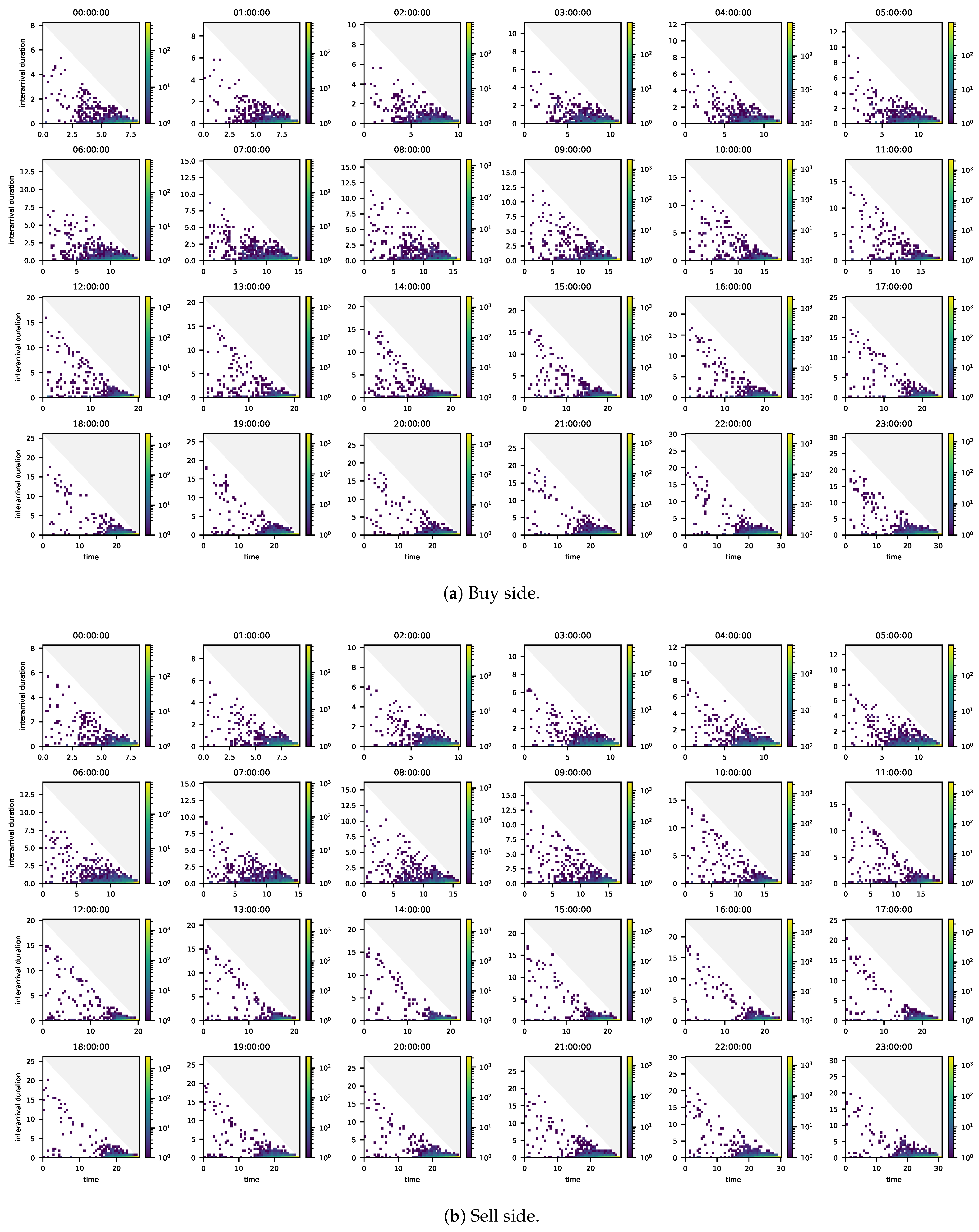
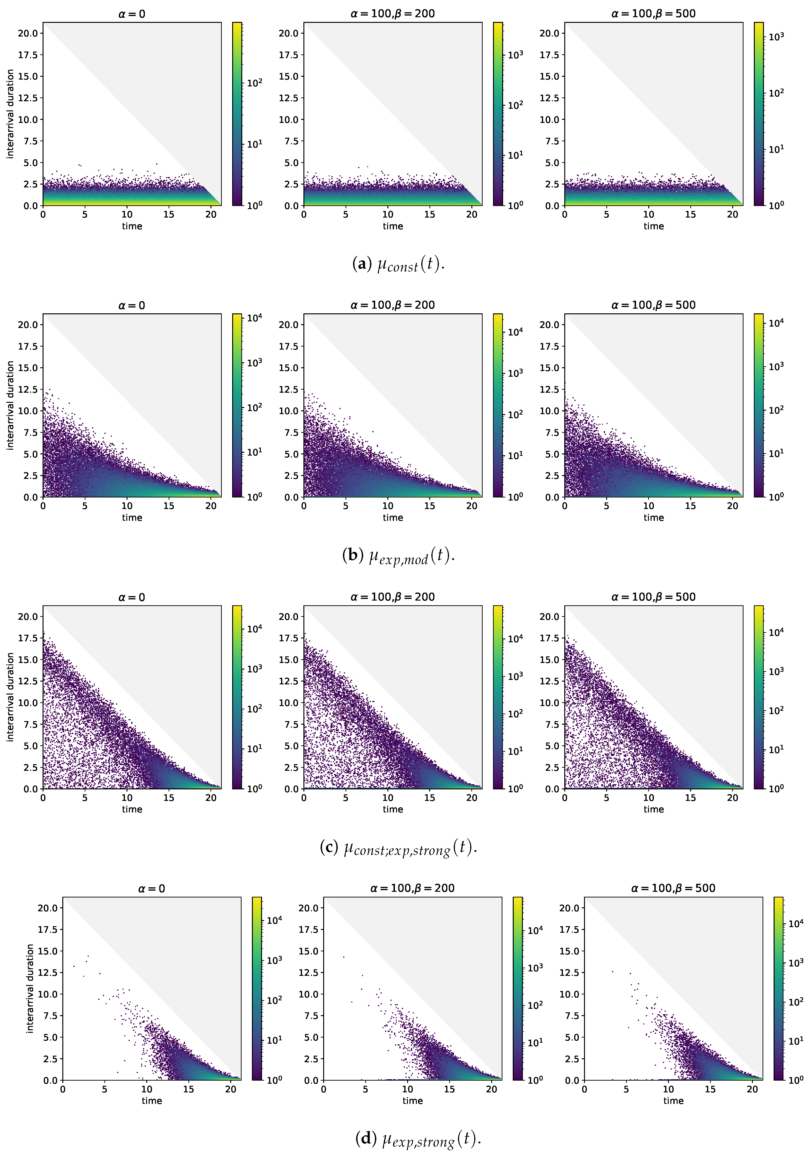
At first, we consider the analysis of arrival times together with interarrival durations. Figure A1 shows the results. Let us consider the case where the (baseline) intensity is constant, see Figure A1a. The event arrivals are distributed equally over time. The bin in which the shortest durations between the time of arrival of an event and the subsequent one fall has the highest frequency, no matter what time is considered. The frequencies of the interarrival duration in which the smaller bins, the larger the durations they cover, again no matter what time is considered. Self-excitation does not invalidate these characteristics but it does cause the frequencies of the bins, which cover the shortest durations to increase and the difference between the frequencies of those bins and the following ones to be larger.
Figure A1. Two-dimensional histograms of event arrival times (horizontal axis) and durations between event arrival times and the arrival time of the next event (vertical axis) for different baseline intensities and self-excitation structures. T = 21.25 , N = 10 4 .
Jrfm 14 00161 g0a1
If the (baseline) intensity comprises not only a constant but also a component which grows visibly over the entire period of time under consideration, the interarrival durations which are associated with arrival times close to t = 0 take values in the region of 12.5 h, see Figure A1b. While these durations are much larger than the maximum durations taken in case of the constant (baseline) intensity, they are also well below the maximum possible durations. With increasing time of arrival, the maximum values that are taken by the interarrival durations decrease. Furthermore, the frequencies of the bins covering small interarrival durations start on increase. As the (baseline) intensity is monotonously increasing, the bins with the highest frequencies are those which are close to t = T and which cover the smallest interarrival durations. The results in case of self-excitation are similar.
What is the effect if the (baseline) intensity also grows exponentially but growth really only becomes noticeable close to t = T ? Figure A1c sheds light on this question. In the hours after t = 0 , a concentration of arrival time-interarrival duration pairs in the region of 8.75 to 3.75 h below the maximum duration may be observed. These pairs are likely to be arrivals that are generated by the constant in the (baseline) intensity and which are followed by arrivals in the phase in which the growth of the (baseline) intensity becomes noticeable. This reasoning is supported by the fact that the arrival time-interarrival duration pairs after t = 0 in case of the (baseline) intensity without a constant are too few to explain the concentration, see Figure A1d. Once again, self-excitation causes the frequencies of the bins covering the short interarrival durations to increase. In Figure A1c, these increases are visible over the entire period under consideration because there are enough events over that period that trigger other events. By contrast, the (baseline) intensity without constant but with strong growth towards t = T does not produce this feature because arrivals after t = 0 fail to occur sufficiently and frequently.
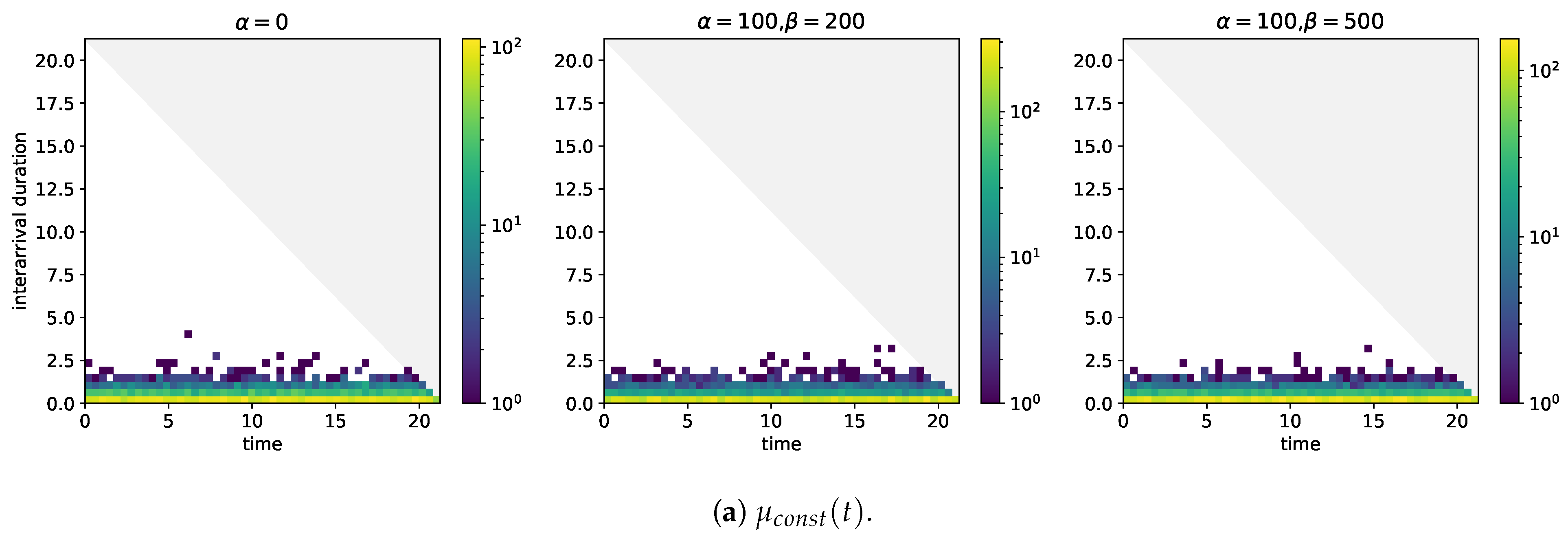
The plots in Figure A1 build upon numbers of observations in the region of 5 × 10 5 and more. With Figure A2 where only 10 2 simulations are included in the analysis of arrival times and interarrival durations, we address the question how the same plots change if less data are available. In the case of the constant (baseline) intensity differences that would be worth mentioning are not observable. A similar conclusion holds in case of the (baseline) intensity that grows visibly over the entire period under consideration and also in case of the (baseline) intensity that grows visibly only close to t = T and that does not comprise a constant. The concentration of arrival time-interarrival duration pairs 8.75 to 3.75 h below the maximum duration, however, is not clearly observable.
Figure A2. Two-dimensional histograms of event arrival times (horizontal axis) and durations between event arrival times and the arrival time of the next event (vertical axis) for different baseline intensities and self-excitation structures. T = 21.25 , N = 10 2 .
Jrfm 14 00161 g0a2aJrfm 14 00161 g0a2b
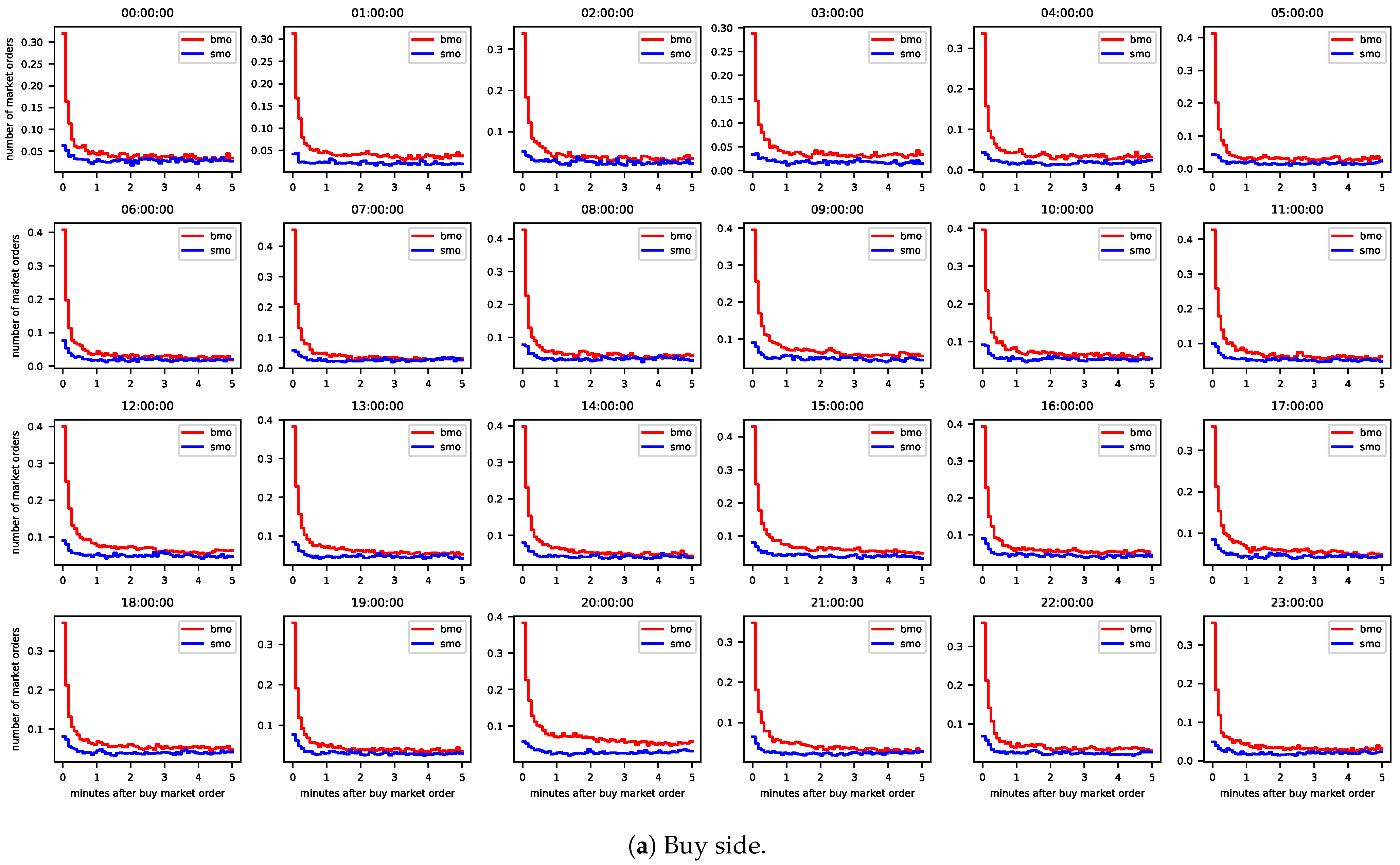
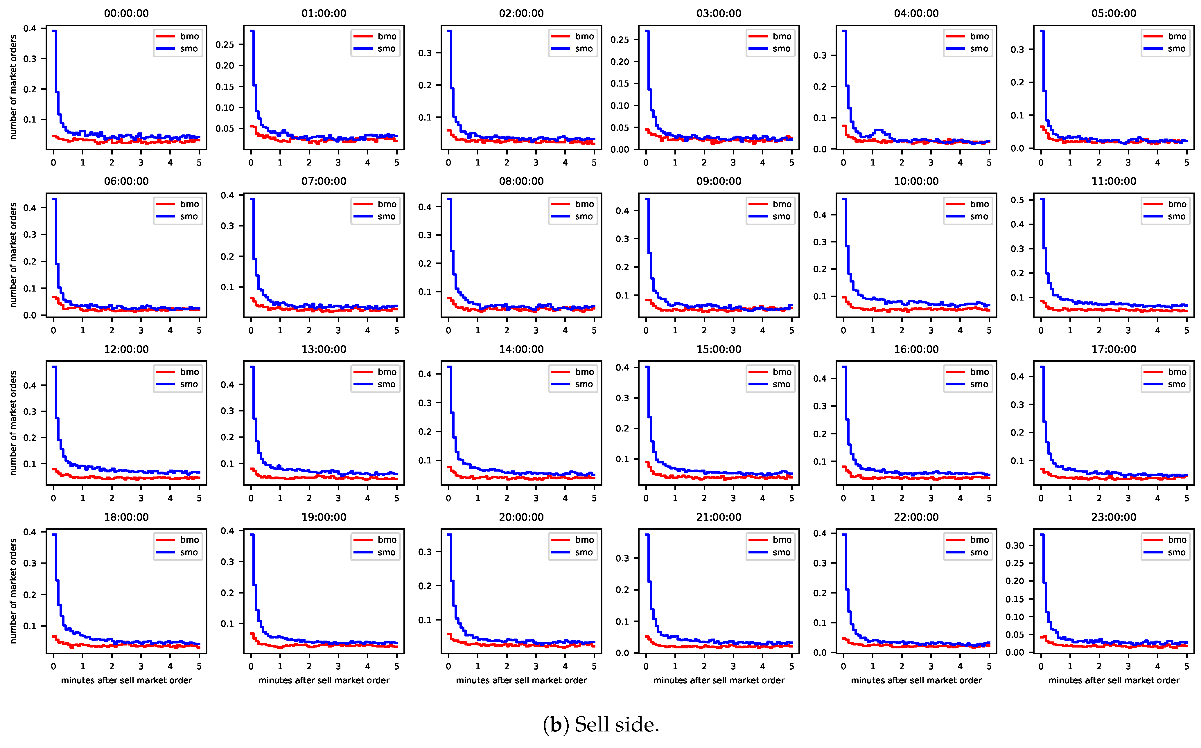
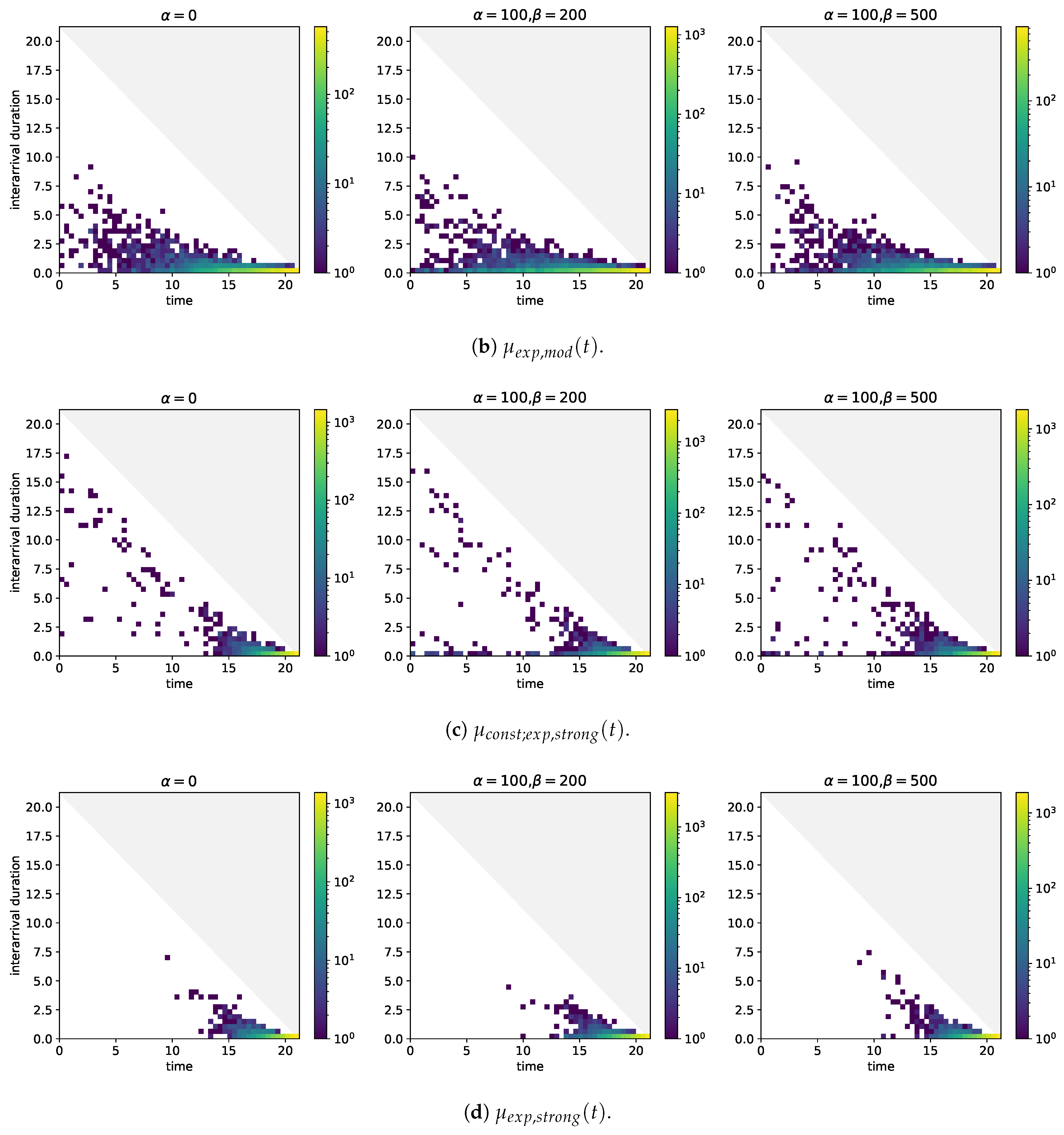
Let us move on to the analysis of the event arrivals that follow the arrival of an event. The results for the 12 models which we also considered in the analysis of arrival times and interarrival durations are shown in Figure A3. If self-excitation is absent, the mean number of events in intervals of 5 s after an event arrival appears to fluctuate randomly around some level, no matter the intensity is, see Figure A3a. In the presence of self-excitation, the mean number of events after an event arrival initially decreases clearly with the increasing distance of the interval, see Figure A3b–d. The amounts by which the means decrease become smaller with the distance of the interval and at some point the means seem only to fluctuate around some level. The initial decline is steeper if β = 500 , i.e., when the branching ratio is smaller. A clear indication that the growth in baseline intensity carries through to the mean number of arrivals after an event arrival is not recognizable.
Figure A3. Mean number of event arrivals in time intervals of 5 s over 5 min after an event arrival. T = 21.25 , N = 10 3 .
Jrfm 14 00161 g0a3

References

  1. Admati, Anat R., and Paul Pfleiderer. 1988. A theory of intraday patterns: Volume and price variability. The Review of Financial Studies 1: 3–40. [Google Scholar] [CrossRef]
  2. Agresti, Alan. 2010. Analysis of Ordinal Categorical Data, 2nd ed. New York: John Wiley & Sons. [Google Scholar]
  3. Bacry, Emmanuel, Iacopo Mastromatteo, and Jean-François Muzy. 2015. Hawkes processes in finance. Market Microstructure and Liquidity 1: 1550005. [Google Scholar] [CrossRef]
  4. Bacry, Emmanuel, and Jean-François Muzy. 2014. Hawkes model for price and trades high-frequency dynamics. Quantitative Finance 14: 1147–66. [Google Scholar] [CrossRef] [Green Version]
  5. Bergsma, Wicher, and Angelos Dassios. 2014. A consistent test of independence based on a sign covariance related to kendall’s tau. Bernoulli 20: 1006–28. [Google Scholar] [CrossRef]
  6. Biais, Bruno, Pierre Hillion, and Chester Spatt. 1995. An empirical analysis of the limit order book and the order flow in the paris bourse. The Journal of Finance 50: 1655–89. [Google Scholar] [CrossRef]
  7. Bowsher, Clive G. 2007. Modelling security market events in continuous time: Intensity based, multivariate point process models. Journal of Econometrics 141: 876–912. [Google Scholar] [CrossRef] [Green Version]
  8. Brémaud, Pierre. 1981. Point Processes and Queues, 1st ed. New York: Springer. [Google Scholar]
  9. Brémaud, Pierre, and Laurent Massoulié. 1996. Stability of nonlinear hawkes processes. The Annals of Probability 24: 1536–88. [Google Scholar] [CrossRef]
  10. Burnham, Kenneth P., and David R. Anderson. 2002. Model Selection and Multimodel Inference: A Practical Information-Theoretic Approach, 2nd ed. New York: Springer. [Google Scholar]
  11. Chen, Feng, and Peter Hall. 2013. Inference for a nonstationary self-exciting point process with an application in ultra-high frequency financial data modeling. Journal of Applied Probability 50: 1006–24. [Google Scholar] [CrossRef]
  12. Chen, Feng, and Tom Stindl. 2018. Direct likelihood evaluation for the renewal hawkes process. Journal of Computational and Graphical Statistics 27: 119–31. [Google Scholar] [CrossRef]
  13. Cox, David R., and Valerie Isham. 1980. Point Processes, 1st ed. London: Chapman and Hall. [Google Scholar]
  14. Da Fonseca, José, and Riadh Zaatour. 2014. Hawkes process: Fast calibration, application to trade clustering and diffusive limit. The Journal of Futures Markets 34: 548–79. [Google Scholar] [CrossRef]
  15. Daley, Daryl J., and David Vere-Jones. 2003. An Introduction to the Theory of Point Processes, 2nd ed. New York: Springer. [Google Scholar]
  16. Easley, David, and Maureen O’Hara. 1992. Time and the process of security price adjustment. The Journal of Finance 47: 577–605. [Google Scholar] [CrossRef]
  17. Engle, Robert F., and Jeffrey R. Russell. 1998. Autoregressive conditional duration: A new model for irregularly spaced transaction data. Econometrica 66: 1127–62. [Google Scholar] [CrossRef]
  18. EPEX SPOT SE. 2020. EPEX Spot Operational Rules. Paris: EPEX SPOT SE. [Google Scholar]
  19. Errais, Eymen, Kay Giesecke, and Lisa R. Goldberg. 2010. Affine point processes and portfolio credit risk. SIAM Journal of Financial Mathematics 1: 642–65. [Google Scholar] [CrossRef] [Green Version]
  20. Eyjolfsson, Heidar, and Dag Tjøstheim. 2018. Self-exciting jump processes with applications to energy markets. Annals of the Institute of Statistical Mathematics 70: 373–93. [Google Scholar] [CrossRef]
  21. Favetto, Benjamin. 2020. The european intraday electricity market: A modeling based on the hawkes process. Journal of Energy Markets 13: 57–96. [Google Scholar]
  22. Gould, Martin D., Mason A. Porter, Stacy Williams, Mark McDonald, Daniel J. Fenn, and Sam D. Howison. 2013. Limit order books. Quantitative Finance 13: 1709–42. [Google Scholar] [CrossRef]
  23. Hawkes, Alan G. 1971. Spectra of some self-exciting and mututally exciting point processes. Biometrika 58: 83–90. [Google Scholar] [CrossRef]
  24. Hawkes, Alan G. 2018. Hawkes processes and their applications to finance: A review. Quantitative Finance 18: 193–98. [Google Scholar] [CrossRef]
  25. Hewlett, Patrick. 2006. Clustering of order arrivals, price impact and trade path optimisation. In Workshop on Financial Modeling with Jump Processes. Palaiseau: Ecole Polytechnique. [Google Scholar]
  26. Jain, Prem C., and Gun-Ho Joh. 1988. The dependence between hourly prices and trading volume. The Journal of Financial and Quantitative Analysis 23: 269–83. [Google Scholar] [CrossRef]
  27. Kramer, Anke, and Rüdiger Kiesel. 2021. Exogenous factors for order arrivals on the intraday electricity market. Energy Economics. forthcoming. [Google Scholar] [CrossRef]
  28. Kremer, Marcel, Rüdiger Kiesel, and Florentina Paraschiv. 2020. A fundamental model for intraday electricity trading. Philosophical Transactions of the Royal Society A. forthcoming. [Google Scholar] [CrossRef]
  29. Lallouache, Mehdi, and Damien Challet. 2016. The limits of statistical significance of hawkes processes fitted to financial data. Quantitative Finance 16: 1–11. [Google Scholar] [CrossRef] [Green Version]
  30. Narajewski, Michal, and Florian Ziel. 2019. Estimation and simulation of the transaction arrival process in intraday electricity markets. Energies 12: 4518. [Google Scholar] [CrossRef] [Green Version]
  31. Rambaldi, Marcello, Emmanuel Bacry, and Fabrizio Lillo. 2017. The role of volume in order book dynamics: A multivariate hawkes process analysis. Quantitative Finance 17: 999–1020. [Google Scholar] [CrossRef]
  32. Scharff, Richard, and Mikael Amelin. 2016. Trading behaviour on the continuous intraday market elbas. Energy Policy 88: 544–557. [Google Scholar] [CrossRef]
Figure 1. Two-dimensional histograms of times at which buy (left) and sell (right) market orders were placed (horizontal axis) and durations between the time at which a market order was placed on one side and the time of the next market order on that side (vertical axis). Data: All contracts with hourly delivery in Q2/2015. For each contract the time at which trading ends is set to the time at which trading ends for the hourly contract with delivery start at 21:00:00 UTC.
Jrfm 14 00161 g001
Figure 2. Mean number of buy and sell market orders in time intervals of 5 s after the arrival of a buy market order (left) and after the arrival of a sell market order (right). Data: All contracts with delivery start at 13:00:00 UTC in Q2/2015.
Jrfm 14 00161 g002aJrfm 14 00161 g002b
Figure 3. Histograms of AIC differences conditional on whether the best model is the one with self-excitation (left) or the one with self and cross-excitation (right). Cases where the AIC difference of the model with self- and cross-excitation is greater than the maximum are removed from the data.
Jrfm 14 00161 g003aJrfm 14 00161 g003b
Figure 4. Median baseline intensity parameters conditional on the hour of delivery start.
Jrfm 14 00161 g004
Figure 5. Median branching ratios conditional on the hour of delivery start.
Jrfm 14 00161 g005
Figure 6. Histograms (diagonal), scatter plots (lower triangle) and two-dimensional histograms (upper triangle) of the parameters of the model with self-excitation.
Jrfm 14 00161 g006
Table 1. Results of goodness-of-fit tests for the marginal processes. The column “side” specifies whether buy or sell market orders (MOs) are considered, “constant” whether the baseline intensity comprises a constant, and “excitation” the excitation structure. Each model is estimated 2184 times. The column “convergence” comprises the shares of successful estimations. The columns “ p K S < 0.05 ” and “ p E D < 0.05 ” comprise the shares of successfully estimated models where the null hypothesis of the Kolmogorov–Smirnov (KS) and excess dispersion (ED) test is rejected at a 5% significance level, respectively. The column “ p L B < 0.05 ” comprises the shares of successfully estimated models where the null hypothesis of the Ljung–Box (LB) test for the first five lags is rejected at a 5% significance level.
a. Individual parameters for each contract.
SideConstantExcitationConvergence p KS < 0.05 p ED < 0.05 p LB < 0.05
buyw/onone96.06%92.42%88.18%13.06%
self95.56%6.13%16.48%7.76%
cross82.92%92.77%87.58%11.98%
self, cross71.29%4.56%13.74%6.42%
withnone87.55%91.68%85.20%11.24%
self83.06%4.96%12.13%6.67%
cross62.77%93.07%84.61%12.98%
self, cross69.23%4.43%9.92%6.42%
sellw/onone97.25%92.94%88.51%14.27%
self96.02%5.15%18.07%8.73%
cross83.10%92.84%87.49%12.18%
self, cross70.88%3.62%13.37%7.17%
withnone87.96%92.45%84.75%12.34%
self84.62%3.63%12.88%7.31%
cross67.08%92.70%85.53%13.45%
self, cross71.75%3.25%10.98%6.89%
b. Equal parameters per hour of delivery.
SideConstantExcitationConvergence p KS < 0.05 p ED < 0.05 p LB < 0.05
buyw/onone100.00%91.03%82.83%15.61%
self100.00%23.95%39.15%10.26%
cross95.83%90.92%83.09%15.53%
self, cross91.67%24.63%39.31%10.04%
withnone100.00%90.34%81.64%15.06%
self95.83%24.51%35.64%9.27%
cross100.00%90.48%81.59%15.48%
self, cross79.17%24.12%36.96%9.31%
sellw/onone100.00%91.76%85.81%17.45%
self100.00%21.11%36.95%10.67%
cross100.00%91.90%85.16%17.08%
self, cross91.67%20.83%36.21%10.39%
withnone100.00%91.39%83.15%16.25%
self100.00%21.70%33.42%9.84%
cross100.00%91.62%82.74%16.35%
self, cross95.83%23.94%33.49%9.89%
Table 2. Results of goodness-of-fit tests for the pooled processes. The columns “constant” and “excitation” under “buy” specify for buy MOs whether the baseline intensity comprises a constant and the excitation structure, analogously for sell MOs. Each model is estimated 2184 times. The column “convergence” comprises the shares where both the model for buy and sell MOs are estimated successfully. The columns “ p K S < 0.05 ” and “ p E D < 0.05 ” comprise the numbers of successfully estimated models in relative terms where the null hypothesis of the KS and ED test is rejected at a 5% significance level, respectively. The column “ p L B < 0.05 ” comprises the numbers of successfully estimated models in relative terms where the null hypothesis of the LB test for the first five lags is rejected at a 5% significance level.
BuySell
Const.ExcitationConst.ExcitationConvergence p KS < 0.05 p ED < 0.05 p LB < 0.05
w/oselfw/oself91.85%3.49%20.94%11.02%
self, cross67.67%3.32%18.13%9.95%
withself80.91%2.43%15.11%10.53%
self, cross68.96%2.86%15.67%10.09%
w/oself, crossw/oself68.73%3.13%18.45%10.13%
self, cross50.09%1.65%15.63%9.32%
withself59.94%2.14%14.06%10.08%
self, cross50.55%1.99%14.22%9.06%
withselfw/oself79.90%2.92%15.13%9.40%
self, cross58.65%2.73%14.44%8.74%
withself70.60%2.20%12.32%10.05%
self, cross59.84%2.30%12.47%9.26%
withself, crossw/oself66.53%3.30%14.38%9.36%
self, cross47.99%2.48%13.17%9.06%
withself59.16%1.93%10.45%8.75%
self, cross50.00%1.56%10.81%8.24%
Table 3. Relative frequencies that the different models are selected on the basis of AIC differences.
a. Without rule of thumb.
SideConstantSelfSelf, Cross
buyw/o47.7%21.1%
with20.6%10.6%
sellw/o45.3%22.9%
with19.7%12.1%
b. With rule of thumb.
SideConstantSelfSelf, Cross
buyw/o74.2%12.4%
with11.2%2.2%
sellw/o72.8%13.3%
with11.4%2.5%
Table 4. Medians of the parameters of the baseline intensity function and the function controlling self- and cross-excitation of buy and sell market order arrivals as well as medians of the branching ratios and half-lifes resulting from these parameters.
BaselineSelfCross
SideConst.Exc. ν γ ˜ η α β α β ln ( 2 ) β α β α β ln ( 2 ) β
buyw/oself 0.230.56173.5479.80.385.20
self, cross 0.250.50169.1518.70.354.8127.2311.20.128.02
withself0.160.050.82204.7562.00.374.44
self, cross0.090.130.63190.1547.10.364.5654.8627.50.093.98
sellw/oself 0.220.56182.1484.50.395.15
self, cross 0.280.44199.3568.40.364.3927.1282.80.118.82
withself0.190.040.85196.2523.90.374.76
self, cross0.100.100.68237.0551.30.394.5347.6585.20.094.26
Table 5. p-values of KS tests with null hypothesis of equally distributed constants, time-zero growth components, and growth rates of the baseline intensity as well as jump sizes and decay rates of self- and cross-excitation.
a. Models for buy side and sell side.
BaselineSelfCross
Const.Excitation ν γ ˜ η α β α β α β α β
w/oself 0.2680.8180.0600.4100.010
self, cross 0.1010.0560.0120.2730.0100.6030.5240.574
withself0.1060.0970.1870.8560.2370.845
self, cross0.2360.7940.7130.1630.7730.4270.7000.4900.773
b. Models without and with constant in baseline intensity.
BaselineSelfCross
SideExcitation γ ˜ η α β α β α β α β
buyself0.0000.0000.0040.0050.065
self, cross0.0100.0000.2130.8120.0990.0000.0040.095
sellself0.0000.0000.0520.0070.003
self, cross0.0030.0000.4670.6940.1560.0110.0010.004
c. Models with self-excitation and models with self and cross-excitation.
BaselineSelf
SideConst. ν γ ˜ η α β α β
buyw/o 0.0910.0000.7200.2270.001
with0.0040.0590.0350.7660.5750.566
sellw/o 0.0080.0000.0100.0030.001
with0.0000.0410.0020.1370.7290.312
Table 6. Kendall’s taus and associated p-values for pairs of parameters of the models with self-excitation.
a. Without constant in baseline intensity.  N = 3052 .
BaselineSelf
γ ˜ η α β α β
baseline γ ˜ 1.000
<0.001
η 0.554 1.000
<0.001<0.001
self α 0.010 0.056 1.000
0.386 <0.001<0.001
β 0.010 0.056 0.769 1.000
0.429 <0.001<0.001<0.001
α β 0.017 0.083 0.042 0.176 1.000
0.161 <0.001<0.001<0.001<0.001
b. With constant in baseline intensity.  N = 482 .
BaselineSelf
ν γ ˜ η α β α β
baseline ν 1.000
<0.001
γ ˜ 0.002 1.000
0.949 <0.001
η 0.071 0.522 1.000
0.020 <0.001<0.001
self α 0.024 0.003 0.012 1.000
0.431 0.934 0.698 <0.001
β 0.033 0.011 0.006 0.693 1.000
0.284 0.730 0.848 <0.001<0.001
α β 0.010 0.022 0.026 0.156 0.106 1.000
0.731 0.466 0.392 <0.001<0.001<0.001
Table 7. Kendall’s taus and associated p-values for pairs of parameters of the models with self- and cross-excitation.
a. Without constant in baseline intensity.  N = 482 .
BaselineSelfCross
γ ˜ η α β α β α β α β
baseline γ ˜ 1.000
<0.001
η 0.438 1.000
<0.001<0.001
self α 0.021 0.106 1.000
0.497 <0.001<0.001
β 0.006 0.107 0.700 1.000
0.853 <0.001<0.001<0.001
α β 0.030 0.049 0.057 0.210 1.000
0.332 0.105 0.060 <0.001<0.001
cross α 0.021 0.179 0.064 0.020 0.081 1.000
0.486 <0.001 0.035 0.521 0.008 <0.001
β 0.001 0.190 0.048 0.014 0.067 0.741 1.000
0.980 <0.001 0.117 0.654 0.028 <0.001<0.001
α β 0.037 0.271 0.017 0.015 0.009 0.274 0.432 1.000
0.219 <0.001 0.571 0.628 0.769 <0.001<0.001<0.001
b. With constant in baseline intensity.  N = 90 .
BaselineSelfCross
ν γ ˜ η α β α β α β α β
basel. ν 1.000
<0.001
γ ˜ 0.251 1.000
<0.001<0.001
η 0.199 0.617 1.000
0.006 <0.001<0.001
self α 0.042 0.040 0.002 1.000
0.558 0.579 0.981 <0.001
β 0.038 0.059 0.039 0.700 1.000
0.598 0.410 0.586 <0.001<0.001
α β 0.109 0.027 0.002 0.184 0.094 1.000
0.132 0.704 0.975 0.010 0.190 <0.001
cross α 0.161 0.092 0.115 0.048 0.112 0.039 1.000
0.026 0.203 0.111 0.505 0.120 0.589 <0.001
β 0.182 0.080 0.120 0.010 0.046 0.051 0.649 1.000
0.012 0.269 0.097 0.892 0.526 0.479 <0.001<0.001
α β 0.001 0.081 0.097 0.022 0.007 0.064 0.113 0.369 1.000
0.989 0.266 0.179 0.756 0.928 0.374 0.117 <0.001<0.001
Table 8. Kendall’s tau and associated p-value for pairs of parameters of the model with self-excitation or the model with self- and cross-excitation for the buy and sell side. N = 1087 .
Sell
BaselineSelf
γ ˜ η α β α β
buybaseline γ ˜ 0.178 0.087 0.003 0.002 0.008
<0.001<0.001 0.867 0.916 0.680
η 0.066 0.266 0.011 0.041 0.058
0.001 <0.001 0.600 0.041 0.004
self α 0.011 0.016 0.043 0.047 0.011
0.576 0.432 0.035 0.021 0.573
β 0.022 0.009 0.029 0.053 0.027
0.276 0.669 0.147 0.009 0.184
α β 0.006 0.062 0.001 0.002 0.018
0.764 0.002 0.965 0.906 0.381
Publisher’s Note: MDPI stays neutral with regard to jurisdictional claims in published maps and institutional affiliations.

