A Comprehensive Statistical Analysis of the Six Major Crypto-Currencies from August 2015 through June 2020

Abstract

After more than a decade of existence, crypto-currencies may now be considered an important class of assets presenting some unique appealing characteristics but also sharing some features with real financial assets. This paper provides a comprehensive statistical analysis of the six most important crypto-currencies from the period 2015–2020. Using daily data we (1) showed that the returns present many of the stylized facts often observed for stock assets, (2) modeled the returns underlying distribution using a semi-parametric mixture model based on the extreme value theory, (3) showed that the returns are weakly autocorrelated and confirmed the presence of long memory as well as short memory in the GARCH volatility, (4) used an econometric approach to compute risk measures, such as the value-at-risk, the expected shortfall, and drawups, (5) found that the crypto-coins’ price trajectories do not contain speculative bubbles and that they move together maintaining the long run equilibrium, and (6) using static and dynamic D-vine pair-copula models, assessed the true dependence structure among the crypto-assets, obtaining robust copula based bivariate dynamic measures of association. The analyses indicate that the strength of dependence among the crypto-currencies has increased over the recent years in the cointegrated crypto-market. The conclusions reached will help investors to manage risk while identifying opportunities for alternative diversified and profitable investments. To complete the analysis we provide a brief discussion on the effects of the COVID-19 pandemic on the crypto-market by including the first semester of 2020 data.

1. Introduction

The crypto-currencies market is a growing volatile market whose dominant element is Bitcoin, a virtual currency created in 2009 by the pseudonymous author Satoshi Nakamoto (Nakamoto 2009). Since then, the number of available crypto-coins has grown steadily and reached over 5500 at the time of writing this paper (see https://coinmarketcap.com/currencies/). Crypto-currencies provide users a fast, secure, and cheap medium of exchange.

Cripto-currencies’ price trajectories may be influenced by a number of factors, including economic and political events, government regulations, the creation of new currencies, speculation, hacking, news, and mutual influence. Relevant players in the crypto-market may be either exercising the currency’s primary utility, which is to pay for goods and services, or looking for alternative profitable investments. They need to be sure that the well known available financial models and financial tools will work with crypto-coins as well. Relevant players’ success will follow from a solid, comprehensive deep understanding of crypto-currencies’ statistical properties, to set their limitations and peculiarities. In particular, volatility and interdependence are two important issues when constructing diversified portfolios and managing risk.

Accordingly, in this paper we clarify many issues related to individual past price and return behavior and co-movements through appropriate statistical tools. Simple models delivered basic statistics and long-run risk measures and predictions. More sophisticated ones such as copula models and cointegration methods uncovered the static and dynamic relationships among crypto-coins, allowing for the simulation of future joint scenarios, and also delivered additional (non-linear) dependence measures.

In the last decade we have seen a growing number of scientific papers taking a formal statistical approach to understanding the dynamics of crypto-coins market prices. For instance, Hencic and Gouriéroux (2015), using a small dataset of 150 observations containing an episode of a speculative bubble, modeled the dynamics of the Bitcoin/USD exchange rate using a non-causal autoregressive process with Cauchy errors. Reference Urquhart (2016) investigated the market efficiency of Bitcoin by employing a battery of robust tests and found evidence of market inefficiency depending upon the sample period. Following that, Nadarajah and Chu (2017) showed that a power transformation of the Bitcoin returns may be weakly market efficient.Reference Urquhart (2017) found significant evidence of clustering of Bitcoin prices at round numbers. In Drożdż et al. (2018) the well known stylized facts were investigated. They showed that by the end of 2017 Bitcoin market had become truly indistinguishable from mature markets according to several statistical features related to the return distribution, such as tail thickness, weak autocorrelation in return distribution, significant (non-linear) long range autocorrelations of absolute value of returns characterizing persistence, and multi-scaling effects. Reference Corbet et al. (2018) provided a systematic review of the empirical literature on crypto-currencies and investigated their role as reliable and legitimate investment assets.

Estimation of crypto-currencies volatilities is a research stream followed by many articles, most of them focusing on Bitcoin dynamics only. Reference Dyhrberg (2016) using GARCH models assessed Bitcoin potential as an asset for risk management and established its role in the market, standing somewhere between a currency and a commodity. However, Cheah and Fry (2015) found that Bitcoin seems to behave more like a speculative asset than a currency. Reference Katsiampa (2017), using the entirety of Bitcoin data since its creation, found which type of GARCH model could better explain the Bitcoin volatility. Reference Chu et al. (2017) modeled the seven most popular crypto-currencies with 12 different GARCH models and computed value at risk (VaR) estimates. Reference Deniz and Stengos (2020) examined the behavior of five crypto-currencies in the pre and post periods of the introduction of the Bitcoin futures market. They found that Google search intensity was the most important variable to explain, for both periods, the BTC mean return (through a PC-LASSO model) and the BTC GARCH volatility.

Long memory in crypto-currencies first and second moments has also been considered by researchers. Reference Bariviera (2017) using data from 2011 to 2017 and moving windows methodology, observed that the time series of Bitcoin’s daily returns exhibited a persistent behavior before 2014, being efficient after 2014; see also Bariviera et al. (2017). Reference Phillip et al (2018) fitted a long memory autorregressive model for the mean combined with a stochastic volatility model with leverage effect and t-student correlated errors to 224 different crypto-currencies. Reference Lahmiri and Bekiros (2018) found that both Bitcoin prices and returns exhibit long-range correlations and multi-fractality. They applied the multi-fractal detrended fluctuation analysis on prices and returns covering two distinct periods, and found that chaos was present in prices during both periods and that heavy tails were the main factor driving the chaos. Reference Garnier and Solna (2018) investigated whether the Bitcoin market can be viewed as a semi-efficient market. They found that Bitcoin exhibits multi-scale correlation structure, and showed how the power-law parameters can be used to identify regime shifts for the Bitcoin price. Reference Tan et al. (2019) applied a structural change model to the top ten crypto-currencies and examined the number and location of change points in daily price, return, and volatility. One conclusion from their research is that the two crypto-currency indices used failed to reflect the whole crypto-currency market.

There has also been some results on crypto-coins’ co-movements. The multivariate GARCH model has been used to assess dynamic interdependence among crypto-currencies. Reference Katsiampa (2019) modeled the volatility and co-volatility of Bitcoin and Ether using an extension of the diagonal BEKK model, thereby finding evidence of interdependencies in the crypto-currency market. Reference Zwick and Syed (2019) applied threshold regression to model the nonlinear long-term relationship among Bitcoin and gold prices. Reference Kristoufek (2015), by applying a wavelet coherency analysis, examined the correlation between Bitcoin prices prices and selected factors. Reference Drożdż et al. (2019) found significant time-scale dependent cross-correlations among BTC/EUR, BTC/US, ETH/EUR, and ETH/US exchange rates at a 10s frequency from July, 2016 to December, 2018. It was also found that the cross-correlations between the BTC/ETH and EUR/USD exchange rates were not significant, probably indicating that the crypto-market has begun to become independent from Forex. As reported in Drożdż et al. (2019), this may be in line with the Drożdż et al. (2018) hypothesis of a gradual emergence of a new and at least partially independent market.

Other related papers are: Ciaian et al. (2016), where the traditional determinants of currency price along with digital currencies specific factors were considered when searching for factors behind the Bitcoin price formation. Reference Li and Wang (2017) examined the determinants of the Bitcoin exchange rate from both technology and economic perspectives. They found that the VECM is not appropriate and applied the ARDL model. Reference Cheah et al. (2018) using cross-market Bitcoin prices from November 2011 to March/2017 found evidence of long memory in the system. However, there is no agreement on the degree of integration of returns and prices, though more empirical evidence has accumulated since 2014.

To the best of our knowledge, this paper is the first one to apply a comprehensive set of statistical modeling approaches—mixtures, ARFIMA-GARCH, pair-copulas, and cointegrated VAR models—to an updated set of the six most important crypto-currencies, plus the Euro, while trying to address several questions: (1) Do prices and returns exhibit some well known characteristics, in particular the famous stylized facts, usually found in financial instruments? (2) Are we able to describe their statistical underlying distributions? (3) Does their dynamic mean and volatility behavior follow the popular univariate/multivariate time series processes usually fitted to financial data, in particular to stock assets? (4) Are there linear and non-linear interdependencies in the crypto-market? (5) Are these crypto-currencies cointegrated? Do prices present speculative bubbles?

Results and findings from this analysis include the specification of a semi-parametric mixture model based on the extreme value theory to represent the returns’ underlying distributions; the confirmation of the presence of long memory as well as short memory in the GARCH volatility, though still leaving as an open question whether long memory in returns may be just anomalies or a period-dependent artifacts; the computation and accuracy assessment of conditional and unconditional risk measures such as the value-at-risk, expected shortfall, and drawups; the rejection of the hypothesis of the existence of explosive bubbles; the description of the true dependence structure among the crypto-assets through static and dynamic (easy to simulate) copula models—through copula-based bivariate dynamic measures of association, we found that the six analyzed crypto-coins are highly linearly and non-linearly correlated with measures which increase over time independently whether experiencing normal or atypical periods; and through the assessment of their dynamic interdependence with cointegration methods, we found a weakly cointegrated market and no empirical evidence for the existence speculative bubbles. The conclusions reached enable an investor to have a broader view of crypto-assets’ behavior, so manage risks while identifying opportunities for more profitable investments. We recall that no good answer or wise decision can be reached if based on a poor model.

The remaining of the paper is organized as follows: In Section 2 we provide a brief description of the six crypto-coins used in this paper and describe the basic statistical analyses. In Section 3 we fit the conditional and unconditional models, thereby obtaining the corresponding risk measures. Section 4 deals with the interdependencies in the data (we applied copula and cointegration methods). Finally, Section 5 discusses the results and provides an extra analysis of the behavior of series during the COVID-19 pandemic.

2. Basic Statistical Analyses

The data in this work are from six virtual currencies: Bitcoin, Ethereum, Ripple, Litecoin, Stellar, and Monero. They were chosen based on their market capitalization rankings provided by CoinMarketCap in 31 January 2020, and they altogether represented approximately 77.4% of the total market capitalization at that time. The percentages of each one were: Bitcoin: 62.2%, Ethereum: 9.8%, Ripple: 3.2%, Litecoin: 1.0%, Stellar: 0.7%, and Monero: 0.5%. In what follows we provide a brief description of the six crypto-currencies.

Designed to be an alternative currency and medium of exchange, Bitcoin (BTC) has shown the largest market capitalization since its creation. As of January 2020 the total available bitcoins were valued at over 171 billion US dollars. Based on cryptographic proves, it is a peer-to-peer based system with online non-centralized public transactions recorded in an “accounting book” known as blockchain. The chain is controlled by its users and follows a set of rules that minimize the probability of fraud. By offering large returns, it has gradually become a speculative investment. See, for example, Baur et al. (2017) where it is discussed whether Bitcoin is mainly used as a currency to pay for goods and services or as an alternative investment. Using daily data from 2010 to 2015, they found that the Bitcoin returns are linearly uncorrelated with all assets both in normal and extreme times, providing diversification opportunities.

Ethereum (ETH), the second-largest digital currency, was conceived by the computer programmer Vitalik Buterin in 2013 (Buterin 2013). It is a computer code (smart contracts) open platform where decentralized peer-to-peer applications run exactly as they were programmed, eliminating the possibility of fraud or any type of interference. As such, Ethereum and Bitcoin blockchain technology purposes are different, as the latter is used to validate transactions among Bitcoin ownerships.

The Ripple crypto-currency (XRP), released in 2012, is the fastest digital asset used by banks to execute end-to-end payments in real time with low transaction costs, independently of amounts transferred and geographic location. XRP important players benefit from its liquidity and faster inter-banking payments: the network takes about four seconds to confirm transactions. Ripple’s activities do not rely on blockchains (as Bitcoin does); the mining is replaced by the work executed by the nodes which listen other nodes for at least 80% confirmation from validators listed in a unique node list.

The globally decentralized digital currency Litecoin (LTC), one of the first Bitcoin forks, was created in 2011 as a "lighter" alternative to Bitcoin. The LTC open source protocol follows the same Bitcoin blockchain concept with a different, four-times-faster hashing algorithm. At the time of this analysis it is the 9th largest digital currency for transferring funds between individuals or businesses in the market with a market cap of over $2.8 billion dollars.

Stellar (XLM), a fork of XRP, was created by Jed McCaleb and Joyce Kim in 2014 and uses the ripple consensus algorithm. Later on, the XLM coin was recreated as an independent foundation, and in 2015 it started using the federated Byzantine agreement algorithm, based on quorum slices, to approve transactions. The Stellar network is really fast with all nodes being updated every 2 to 5 s. It is the most decentralized open source not-minable network, able to trade any fiat or crypto-currency, asset, or token around the world. The motivation behind its creation was the reduction of costs required for cross-border transfers, and it has been used for small payments within a company or among private entities as well as for currency exchange. The Stellar technology may be used for building new applications, and connecting banks and people. The XLM’s price showed a significant increase in May, 2017, and another jump in November of the same year, but presented an downward trend (shared by all other crypto-currencies) during all second semester of 2019.

Monero (XMR) launched on April 2014, is a proof-of-work secure decentralized crypto-currency operated by a network of users which uses ring signatures (a type of digital signature), ring confidential transactions, and stealth addresses (this prevents address reuse since only the sender and receiver of a transaction can determine where a payment is to be sent). Monero is untraceable; that is, the transactions recorded on the blockchain cannot be linked to any particular user, and also exchangeable (fungible): 1 XMR is functionally identical to any other 1 XMR. Differently from Bitcoin, which is a transparent network, Monero has strong privacy properties, able to hide information on the amount of money sent from one user to another in all transactions.

The six series were obtained from the Quandl’s platform (www.quandl.com). For each currency we selected its BraveNewCoin daily global price index (BNC2) recorded in USD each 5-min and based on an aggregate of all transactions for that coin at that time. For the sake of comparisons we also included the Euro. Series cover the period from 8 August 2015 to 31 January 2020, that being the initial date defined by the shortest series, Ethereum. Another reason for not including data since 2009 is the different dynamic behavior of the existing crypto-currencies during the initial existence of the crypto-market (2009–2014), which would affect the robustness of the statistical estimates resulting in poor, unreliable conclusions. Note that some authors have demonstrated that the crypto-currency market in its infancy was inefficientm not following the efficient market hypothesis (EMH), being ruled by a different underlying statistical model; see, for example, Urquhart (2016) and Bariviera (2017), among others.

Let $P_t$ denote the crypto-currencies prices in US Dollar at time t. The corresponding log-return $r_t$ is computed as $r_t=100\ast log\left(\frac{P_t}{P_{t-1}}\right)$. Length of all crypto-currencies log-returns series is $T=1637$, whereas the Euro series has length 1146.

Most stylized facts often observed in financial returns series (in particular stocks and indexes) were also noticed for the crypto-assets returns (Engle and Patton 2001; Cont 2001; Tsay 2002; Drożdż et al. 2018). Some of these features were observed graphically and confirmed by usual statistical tests at the 1% significance level. All return series are second order stationary (KPSS test, Kwiatkowski et al. 1992) with a constant level close to zero, whereas the corresponding price series are nonstationary possessing a unit-root (ADF and PP tests, Dickey and Fuller 1979; Phillips and Perron 1988). 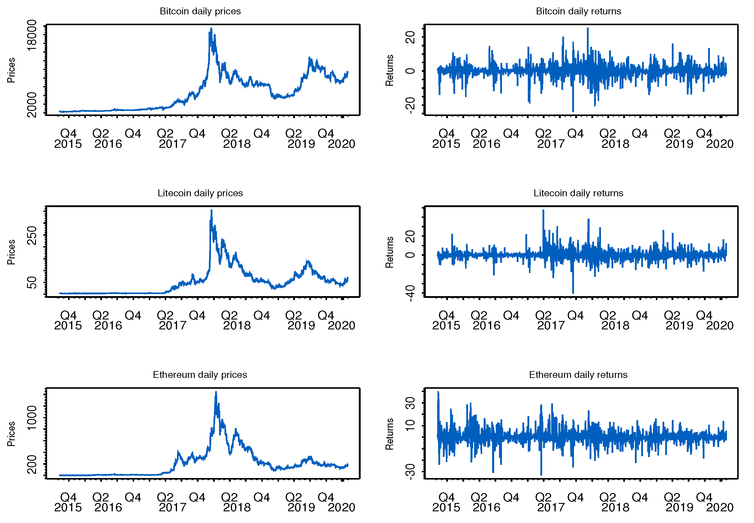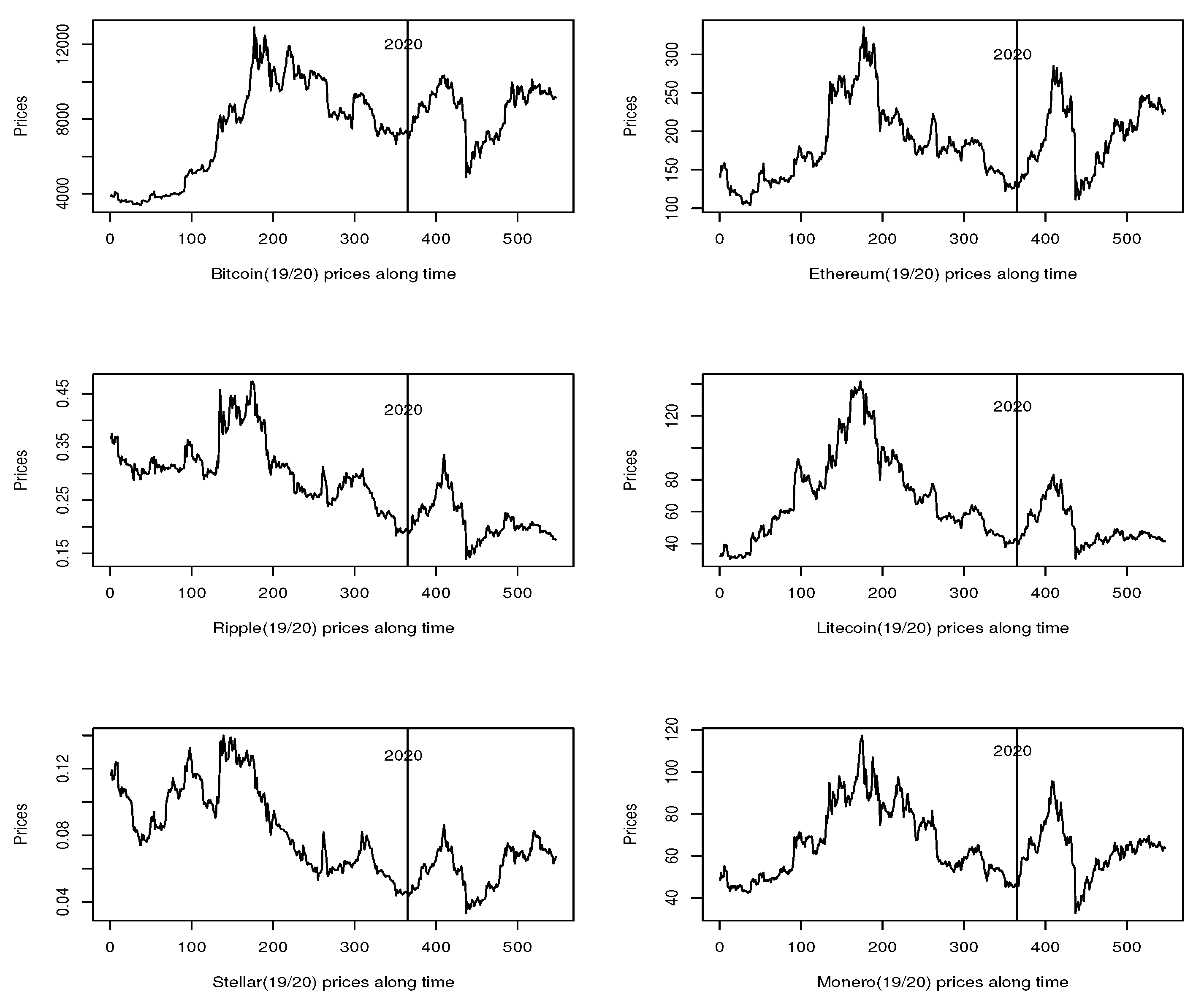Figure 1 illustrates and shows the (price and return) series dynamics of Bitcoin, Litecoin, and Ethereum, with returns showing volatility clusters (conditional heteroscedasticity) and a few extreme points. We also observe in Figure 1 that the price trajectories seem to move together, presenting joint episodes of runs of increasing prices (or sequences of positive returns) followed by corrections (in Section 3 we investigate if they could actually be speculative bubbles), suggesting that joint co-movements and measures of association are worth investigating.

Table 1. Returns basic statistics. (Notation in table: * means 5% statistical significance).

	Bitcoin	Ethereum	Ripple	Litecoin	Stellar	Monero	Euro
Mean	0.21	0.34	0.20	0.17	0.19	0.29	0.00
0.99%[LCL, UCL]	[−0.03,0.47]	[−0.06,0.74]	[−0.25,0.66]	[−0.17,0.52]	[−0.90,1.30]	[−0.14,0.71]	[−0.04,0.04]
Median	0.23	−0.06	−0.30	−0.05	−0.36	−0.07	−0.01
Standard deviation	3.96	6.33	7.18	5.49	17.37	6.60	0.48
Maximum	25.49	39.94	101.97	47.97	269.14	56.47	2.47
Minimum	−23.97	−33.35	−63.15	−40.60	−244.65	−29.18	−2.88
Skewness	−0.21 *	0.43 *	2.60 *	1.02 *	0.06	0.93 *	0.12
Kurtosis	5.55	5.22	36.75	11.41	83.51	7.46	3.43

provides some summary statistics for all seven returns series. Although the sample means for all crypto-currencies are positive, the t-test null of a true mean equal to zero was accepted at the 1% significance level for all return series. The second row provides the lower and upper 99% confidence limits for the sample mean. Returns from all seven series are not normally distributed, as confirmed by the Jarque–Bera and Shapiro–Wilk tests with p-values close to zero. Stellar has the largest standard deviation, the largest maximum, and the smallest minimum. All the very extreme points observed for Stellar occurred at the beginning of the series (2016), with the recent part of the series showing a much smaller range. When compared to Euro, all crypto-assets show larger standard deviations and also more extreme minimum and maximum.

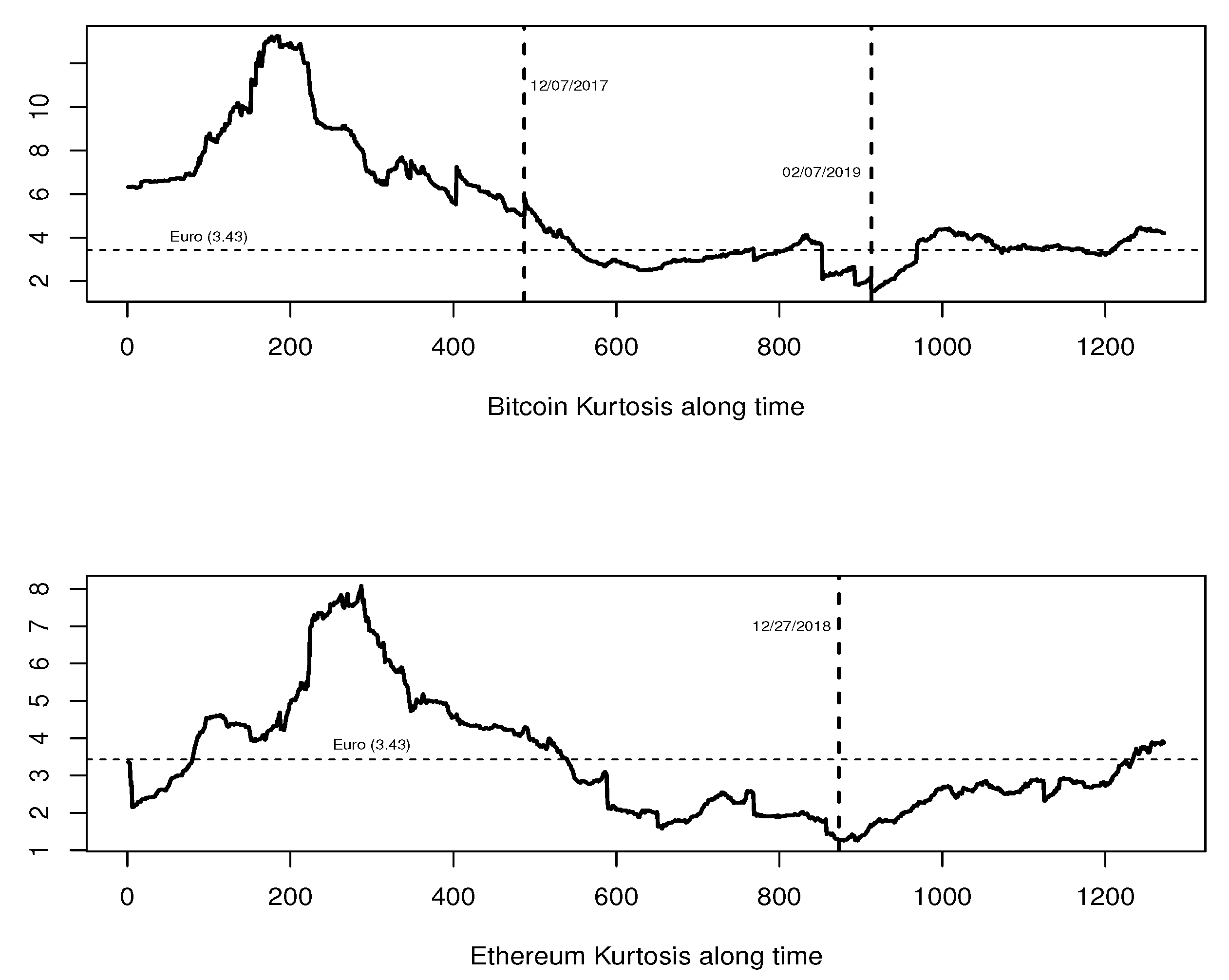
Kurtosis coefficients larger than 3 were observed for all series. As pointed out by an anonymous referee, these results are in fact consistent with Drożdż et al. (2018) where, according to the Hurst exponent, the Bitcoin return distribution tail thickness has decreased over the 2016–2017 years, indicating that Bitcoin may be approaching a mature state. As suggested by this referee, we dynamically examined through a one-year rolling window, the Bitcoin and Ethereum kurtosis evolution from August 2015 to January 2020. In Figure 2 we see that Bitcoin kurtosis reaches the 5.0 level by middle 2017 and continues going down even below the 3.43 mean level observed for Euro. Bitcoin kurtosis reaches its smaller value (1.524) around 7 February 2019. For Ethereum, the kurtosis values are even smaller, staying bellow the Euro mean level during 2018–2019. The systematic decrease of the Bitcoin and Ethereum kurtosis to the Euro mean level depicted in Figure 2 are in line with results in Drożdż et al. (2018), and might be an indication that most important virtual coins are on their route to maturity.

For all crypto-currency returns, the minimum is less extreme than the maximum. Coherently, all crypto-assets, except Bitcoin, yielded positive skewness coefficients. Bitcoin’s coefficient of asymmetry was negative and statistically significant. For all crypto-assets, except Bitcoin, we observed a negative median and a positive mean, suggesting the influence of some extreme positive returns shifting the sample mean to the right. Bitcoin’s (statistically zero) mean and median are both positive and close, indicating that no extreme points affected the computation of the sample mean. Subsequently, we reject that the returns’ distribution is symmetric, except for Stellar and Euro. Is the left tail (negative returns) of Bitcoin heavier than the right tail? Are Bitcoin’s losses more likely than its gains? We provide answers to these questions in the next section.

According to the Ljung–Box test, for all digital assets the linear correlations among lagged returns are either statistically zero or weak for just the first lags. However, the squared returns series showed significant correlation coefficients at small lags, although not as remarkable as those observed for stocks or stock indexes. For all series there is no evidence of long-memory (R/S test) in the mean.

3. Assessing Crypto-Assets’ Risks

To assess risk we computed the most popular risk measure value-at-risk (VaR) and the conditional VaR (Tsay 2002). For small $\alpha$ the VaR${}_{\alpha }$ may be defined as the $(1-\alpha )$%-quantile of the returns’ distribution F; and the conditional VaR${}_{\alpha }$ is the expected loss (EL${}_{\alpha }$), the mean return larger than the VaR value—that is, $E[r_t-\mathrm{VaR}{}_{\alpha }|r_t>\mathrm{VaR}{}_{\alpha }]$ (both defined in the right tail).

3.1. Unconditional Risk

Risks associated with long term investments are better assessed by unconditional risk measures, and to obtain accurate risk estimates it is crucial to find the best estimate for the underlying distribution F of each returns series. All probabilistic aspects already commented on—long heavy tails, asymmetry, very large kurtosis, and extreme outliers—suggest that no single statistical distribution would be able to describe, with some degree of accuracy, the entire range of data. For example, Chan et al. (2017) fitted eight parametric distributions to the historical returns of seven crypto-currencies’ global indices, and found that they are not normally distributed, and moreover, no single distribution fits all the series well.

Despite all the evidence, we tried to fit potential candidates to the data, namely, the normal, the student-t, and three versions of the skew-t (Hansen 1994: Jones and Faddy 2003, and Zhu and Galbraith 2010). They all failed to accepted the Kolmogorov–Smirnoff null of a good fit (goodness of fit test, GOF). The only exception was the Euro accepting the normal and the student-t as possible models. By noting that risk is mainly concerned with tail behavior, in this paper we propose fitting a mixture model (McLachlan and Peel 2000) based on a extreme value distribution to the historical returns. We fit the generalized Pareto distribution (GPD) (Pickands 1975; de Haan 1984; McNeil and Frey 2000) to the excesses $(r_t-u)$ beyond a high threshold u (on each tail), and estimated the bulk of the data using the empirical distribution. Therefore, we combined three distributions to represent the data.

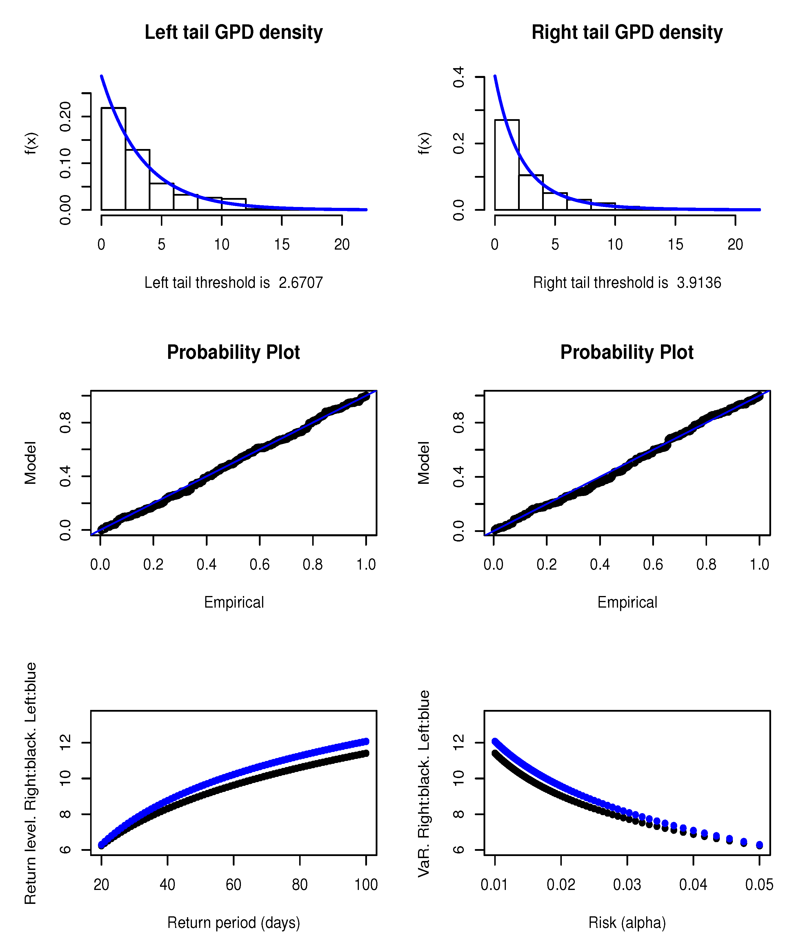
The thresholds were defined as the return value in the tail defining a small percentage $p^{*}$ of extreme values, and $p^{*}$ was chosen as the proportion resulting in the best GPD fit for the excesses. The empirical distribution of the excesses was also graphically checked for a strictly decreasing shape. We were able to find excellent maximum likelihood fits (Hosking and Wallis 1987; Hosking and Wallis 1997) for both tails of all series, accepted by the GOF test and confirmed by graphical diagnosis such as the QQ-plot and the PP-plot. For instance, see the first and second rows of Figure 3 where we show, for both tails, the excellent adherence of the GPD to the Bitcoin excess data.

Table 2. GPD estimates and long-run risk measures: shape parameter (standard error); percentage of excesses $p^{*}$; 1% and 5% VaR and expected loss (EL) estimates.

Estimates	Bitcoin	Ethereum	Ripple	Litecoin	Stellar	Monero	Euro
Left tail estimates
Shape(st. er); $p^{*}$	0.02(0.07); 14%	0.04(0.08); 13%	0.25(0.10); 10%	0.12(0.08); 12%	0.59(0.10); 15%	0.01(0.07); 17%	0.20(0.11); 9%
VaR: 1% & 5%	−12.08 & −6.29	−17.56 & −9.50	−16.91 & −8.29	−14.29 & −7.64	−39.13 & −13.40	−16.67 & −9.63	−1.18 & −0.71
EL: 1% & 5%	15.24 & 10.03	23.04 & 14.75	24.48 & 14.15	20.70 & 12.14	89.38 & 35.66	20.41 & 14.10	1.75 & 1.00
Right tail estimates
Shape(st. er); $p^{*}$	0.15(0.09); 12%	0.00(0.06); 13%	0.33(0.12); 9%	0.21(0.08); 14%	0.57(0.12); 11%	0.15(0.07); 16%	0.24(0.13); 8%
VaR: 5% & 1%	6.23 & 11.41	11.15 & 20.23	10.06 & 24.61	8.63 & 18.00	15.68 & 46.98	10.83 & 20.60	0.76 & 1.25
EL: 5% & 1%	9.78 & 14.81	16.84 & 27.93	19.81 & 39.91	15.43 & 27.75	38.74 & 86.72	16.91 & 30.10	1.07 & 1.83

gathers results from the GPD fits using the entire sample of 1637 observations. The first row shows the estimates of the shape parameter, the standard error, and the proportion $p^{*}$ of tail data used in the estimation process. All estimates of the shape parameter were positive, indicating a Pareto type distribution. However, half of them were statistically zero (exponential tail) at the 5% significance level: both tails of Bitcoin, Ethereum, Euro; and also Litecoin and Monero left tails. The proportions $p^{*}$ were higher than those suggested by text books, ranging from 8% to 17%, probably due to the long tails and the presence of some atypical extreme points.

The VaR estimation based on a GPD fit was expected to be much more precise, since it is based on a less extreme GPD quantile. More specifically, the GPD based VaR${}_{\alpha }$ is equal to $u+{\mathrm{GPD}}^{-1}(1-\frac{\alpha }{p^{*}})$, where ${\mathrm{GPD}}^{-1}$ denotes the quantile function of a GPD. The second row of each panel of Table 2 provides the VaR estimates for $\alpha$ equal to $0.05$ and $0.01$. For all crypto-currencies we checked whether the risk associated to the estimated VaR was actually $\alpha$ by applying the Kupiek test, which accepted the null for both tails and for both risk levels, at the 5% significance level.

When comparing in Table 2, the values of the risk measures, we note that the right tail is riskier than the left tail for all series except for Bitcoin, meaning that with the same probability $\alpha$, only for Bitcoin, the losses may be larger than gains. Bitcoin shows, in addition, smaller risk estimates. For example, a one-percent chance the BTC log-returns will be less than −12.08%, whereas ETH log-returns should be less than −17.56%. While trying to answer the questions raised in Section 2, we now collect several indications that the Bitcoin left tail is actually heavier than the right one: the negative coefficient of asymmetry, the risk measures in Table 2, and the slower decay rate of the estimated left tail GPD density (see first row of Figure 3). The GPD fit indeed sheds light on what is happening at the tails, providing more accurate risk measures, and in the case of Bitcoin, it is robust and not affected by the longer right tail caused by the extreme maximum.

For all series and for $\alpha =0.05$, the historical and the normal VaR (not reported here) were close to the GPD values. However, for $\alpha =0.01$, the assumption of normality severely underestimated the risk measures. For example, the Bitcoin VaR${}_{0.01}$ under normality would be −9.00 and 9.43. Like stocks and indexes, it seems that simple methods based on normality will not work with crypto-assets.

Many practitioners seem to prefer working with the concept of “return level,” instead of reporting the VaR value. The return level (RL) is defined as ${\mathrm{RL}}_t=F^{-1}(1-1/t)$; that is, a value which is expected to observe with some regularity, the return period t. For example, let $t=100$ days. The ${\mathrm{RL}}_{100}$ is equal to the 1% VaR, an event that happens on average once each 100 days. The third row of Figure 3 shows for both tails of Bitcoin, the ${\mathrm{RL}}_t$ for $t=20,\cdots ,100$ on the left-hand side, and the corresponding $\alpha$% VaR for $\alpha =0.01,\cdots ,0.05$, on the right-hand side. As discussed above, we note that the left tail of Bitcoin (in blue) is riskier than the right tail.

To assess the impacts of recent observations on the unconditional risk measures, we carried on a rolling window exercise. We separated an initial sample of 730 observations (two years), estimated the GPD models, and computed the risk measures. Then, the window moved 1 d ahead and the whole procedure was repeated until the end of the sample (1637 observations) was reached. For all crypto-currencies, we observed no trends or fluctuations of the dynamic VaR estimates around the unconditional estimate, but a small distance from (above or below) the fixed reported value. The rolling window values were more accurate, in the sense that even though the proportion of violations was pretty much the same, the expected loss values were smaller. The GOF and the Kupiek tests accepted their nulls for the results from all 907 windows. It seems that a two-year sample is able to provide a very good GPD fit and therefore accurate updated risk estimates.

Finally, to have a broader view of the crypto-assets’ unconditional risks, we mention a different type of risk provided by a sequence of (consecutive) negative or positive returns, the so called drawdowns, or drawups. A drawdown (drawup) is a risk measure given by the sum of the consecutive losses (gains), whose duration is also a random variable. Note that a drawdown may not be extreme but may possess a large duration, and some investors following closely the performance of their investments, may not stand for a long period of successive losses, withdrawing from the market.

The empirical probability distribution of the duration was similar for all crypto-assets, and also similar to what is observed for stock assets. Typically, around 48% of drawdowns and drawups lasted for one day; 24% had a length of two days; and 0.5% lasted for 9 or 10 days.

For all crypto-coins the amount of accumulated gains was larger than the sum of consecutive losses. Even though the Bitcoin values were smaller, they were ten to twenty times greater than the numbers for the Euro. There is no link between sizes and durations; for example, whereas the largest accumulated gain for Bitcoin (63%) lasted eight days, it took only two days for Stellar produce its largest drawup (272%). The largest Bitcoin drawup was initiated on 30 November 2017, and it is interesting to note that a few days later both LTC and ETH presented sequences of extreme gains.

Drawups and drawdowns may also be defined, and better visualized on the price trajectories: it is just a run of increasing (decreasing) prices. In this context drawups may be identified as bubbles (Cheah and Fry 2015; Fry and Cheah 2016). According to the dependence test (McQueen and Thorley 1994), speculative bubbles should exhibit negative duration dependence. This test assumes that during the existence of a drawup the conditional probability that a run ends decreases with time. For instance, Chan and Laurini (2018) found evidence for the absence of any bubble in Bitcoin in 2017. For our data we found no significant empirical evidence of speculative bubbles. This result is important because in Section 4.2 we apply cointegration methods are used to assess interdependence, and the model requires that the observed co-movements are not driven by speculative bubbles.

3.2. Conditional Risk

Dynamic unsystematic risk may be accurately estimated at some point in the near future through econometric model-based conditional measures. In this paper we fit the ARFIMA$(p,d,q)$-FIGARCH$(m,D,s)$ (autoregressive fractionally integrated moving average-fractionally integrated generalized autoregressive conditionally heteroskedastic) model to the crypto-assets returns, a powerful combination of short and long memory conditional models for the mean and for the volatility. The ARFIMA-GARCH model may be written as

$$\Phi \left(B\right){(1-B)}^d{r}_t=\Theta \left(B\right)a_t,d\in \Re ,$$

(1)

where the polynomial $\Phi \left(B\right)$ and $\Theta \left(B\right)$ are of orders p and q, respectively, the fractional differentiation (see Hosking 1981) is given by the term ${(1-B)}^d$, and the white noise process ${\left\{a_t\right\}}_{t\in Z}$ has zero mean and finite variance. It is assumed that $a_t=\sqrt{{\sigma }_t^2}{\epsilon }_t$, and the conditional variance is specified as

$${\sigma }_t^2=\omega +{\alpha }_1{a}_{t-1}^2+\cdots +{\alpha }_m{a}_{t-m}^2+{\beta }_1{\sigma }_{t-1}^2+{\beta }_2{\sigma }_{t-2}^2+\cdots +{\beta }_s{\sigma }_{t-s}^2,$$

(2)

with $\left\{{\epsilon }_t\right\}\sim \mathrm{i.i.d.}F(0,1)$. The volatility Equation (2) may me extended to include the long memory parameter D, see Baillie et al. (1996) and Bollerslev and Mikkelsen (1996).

Our model estimation approach is top-down: We consider the full model, which, step by step, is reduced by the elimination of parameters not statistically significant. The initial orders $(p,q,m,s)$ are suggested by the examination of the autocorrelation functions and by the application of the Ljung–Box and ARCH tests. The AIC criterion helps selecting the best model for each series. The good quality of fit is then verified through diagnosis plots and formal tests applied to the residuals. Models were fitted to the entire sample except in the case of Stellar, which showed a turbulent initial period (completely different from the rest of the sample) with very high volatility affecting the convergence of algorithms. For this series the first 160 observations were removed. Their atypical influence may be proved by the statistics (standard deviation, maximum, minimum), which were computed for the removed initial period and the remaining sample produced, respectively, provided the values (50.35, 269.14, −244.65) and (7.84, 72.41, −37.56).

Table 3. Summary of the results from the ARFIMA$(p,d,q)$-FIGARCH$(m,D,s)$ fits for all series. All parameters estimates are 5% statistically significant. Notations: LEV: leverage parameter; d.f.: degrees of freedom of the F distribution; skew: skewness estimate of the skew-t distribution.

Crypto-Coin	$({\mathit{\varphi }}_0,{\mathit{\varphi }}_1)$	d	${\mathit{\theta }}_1$	$\mathit{\omega }$	${\mathit{\alpha }}_1$	D	${\mathit{\beta }}_1$	${\mathit{\beta }}_2$	LEV	d.f.	Skew	AIC	1%-VaR
Bitcoin-LM	(0.201,–)	0.00	—	0.144	0.258	0.689	0.780	—	—	3.15	—	5.0577	(−6.80,7.20)
Bitcoin	(0.207,–)	0.00	—	0.212	0.225	—	0.401	0.418	−0.089	3.11	—	5.0584	(−7.23,7.65)
Ethereum-LM	(0.128,–)	0.00	—	3.470	0.138	0.646	0.515	—	—	3.18	1.064	6.1096	(−10.59,12.05)
Ethereum	(0.128,–)	0.00	—	2.726	0.261	—	0.738	—	—	3.08	1.063	6.1116	(−11.28,12.82)
Ripple-LM	(−0.156,–)	0.00	−0.154	0.623	0.678	0.451	0.744	—	—	2.81	1.065	5.7761	(−7.58,8.56)
Ripple	(−0.160,–)	0.00	−0.154	2.059	0.263	—	0.736	—	—	2.72	1.056	5.7967	(−8.99,10.01)
Litecoin-LM	(–,–)	0.00	—	0.001	0.361	0.619	0.753	—	—	3.11	1.048	5.5577	(−11.79,12.80)
Litecoin	(–,–)	0.00	—	0.092	0.107	—	0.892	—	—	3.10	1.045	5.5676	(−13.68,14.77)
Stellar-LM	(–,–)	0.00	−0.097	0.815	0.278	0.374	0.375	—	—	3.47	1.143	6.2334	(−9.61,11.65)
Stellar	(–,–)	0.00	−0.093	1.801	0.212	—	0.787	—	—	3.17	1.133	6.2541	(−9.75,11.86)
Monero-LM	(–,–)	0.0	−0.110	3.256	0.115	0.652	0.582	—	—	3.30	1.056	6.2455	(−12.40,14.33)
Monero	(–,–)	0.00	−0.110	2.321	0.206	—	0.793	—	—	3.18	1.053	6.2472	(−13.14,15.09)
Euro-LM	(–,–)	0.00	—	0.002	0.043	0.503	0.274	0.484	—	4.82	—	1.4120	(−0.78,0.78)
Euro	(–,–)	0.00	—	0.001	0.019	—	0.975	—	—	6.73	1.088	1.2403	(−0.79,0.88)

provides a summary of the best fits found for all seven series. Choices considered for the error distribution F were the normal, the t-student, and the skew-t. An important extension of the GARCH model including the leverage parameter (information asymmetry) was also considered. It was significant only for Bitcoin which showed, as expected, a negative value, indicating that negative returns increase volatility. Long memory in the mean was not detected for all return series, but it was strong in the volatility (around 0.6 for all series). According to the AIC value, for all crypto-currencies the fractionally integrated FIGARCH won over the version without long memory in the volatility. We report the two solutions in Table 3.

Bitcoin differentiates itself from all other crypto-coins in at least three aspects. It is the only one to include in the best model the leverage effect (LEV), to include the ${\beta }_2$ term, and to have the (symmetric) student-t as the error distribution F. Bitcoin, Ethereum, Litecoin, and Euro did not present short memory in the mean ($p=q=0$). For XRP, XLM, and XMR $p=0$ and $q=1$ (see second and fourth columns). The degrees of freedom are very small characterizing heavy tails. In summary, with respect to econometric models, crypto-coins returns behave much like stock returns by presenting the same stylized facts, volatility clusters, high persistence, and long memory in volatility—substantially differing, however, in tail weight; see in Table 3 the Euro’s lighter F.

Table 3 also shows in the last column the one-step-ahead conditional 1%-VaR at the left and right tails, computed using the corresponding ARFIMA-GARCH models. The volatility forecasts reflect the low volatility level at the end of the series (see Figure 1).

We estimated and tested the out-of-sample performances of the one-step-ahead conditional risk measures by applying the same already described rolling window approach. At each step the best GARCH model found for each series was fitted to the data inside the window and the next day ${\mathrm{VaR}}_{\alpha }$ was computed using the one-step-ahead predictions for the mean and for the volatility. To assess the performances of the 907 one-day-ahead predictions we applied the Kupiec test to test whether the observed frequencies of VaR exceedances were consistent with the expected ones. The test accepted the null for all series at the 1% level. In summary, like real assets, all crypto-currencies volatilities were well modeled by some type of GARCH model, providing reliable conditional risk measures estimates.

4. A Look at Dependence

Understanding the interdependencies among crypto-currencies is important for those investors looking for portfolio diversification, hedging, and also risk management. Co-movements may be assessed through static models such as copulas, and also dynamically using multivariate time series models. Different models will measure different forms of association, and there is no unique measure to quantify interdependence. For example, Drożdż et al. (2020) studied the cross-correlations among a collection of the 100 highest-capitalization crypto-currencies from 1 October 2015 to 31 March 2019, thereby finding a criterion for identifying which currencies or crypto-currencies are more influential in the crypto-market. They also found evidence of an emergent independence of the crypto-market. In this section we study the dependencies among the six crypto-coins taking two different approaches—to the best of our knowledge not found in the current literature with such a set of crypto-currencies and for this recent period—by estimating their returns’ true copula dependence structures, and investigating their daily price cointegrations.

4.1. Dependence (by Pair-Copulas)

The true extent of dependence between assets tends to be masked by turbulent periods. To assess the true dependence structure linking the crypto-currencies we fit copula models to the standardized residuals from the GARCH fits. The filtered data usually show a weaker degree of dependence when compared to the raw log-returns, and may emphasize the information asymmetry providing different measures for the association in the lower left corner (joint losses) and in the upper right corner (joint gains). The knowledge asymmetric dependence may lead to statistically significant portfolio gains.

Consider the 6-dimensional continuous random vector $(r_1,\cdots ,r_6)$ representing the six crypto-currencies standardized residuals from the econometric models fitted in Section 3.2. Their joint cumulative distribution function (cdf) and density function are respectively given by F and f, $F_i$ ($f_i$) represents the cdf (density function) of $r_i$, and $F_i^{-1}$ stands for the quantile function of $r_i$, $i=1,\cdots ,6$. The copula C associated to F is obtained through the following transformation to a simpler ${[0,1]}^6$ space: $C(u_1,\cdots ,u_6)=F(r_1,\cdots ,r_6)$ where $(u_1,\cdots ,u_6)=(F_1\left(r_1\right),\cdots ,F_6\left(r_6\right))$. The copula C carries all the information about the dependence structure among the corresponding returns (Nelsen 2006).

Copula models provide invariant measures for the strength of dependence between extreme joint values. They are the copula based lower and upper tail dependence coefficients ${\lambda }_L$ and ${\lambda }_U$, defined as ${\lambda }_U={lim}_{u\uparrow 1}\frac{\overline{C}(u,u)}{1-u},\mathrm{where}\overline{C}(u_1,u_2)=P(U_1>u_1,U_2>u_2)$, and ${\lambda }_L={lim}_{u\downarrow 0}\frac{C(u,u)}{u}$, if these limits exist. These tail dependence coefficients (TDC) are highly relevant for risk management, and may be better appreciated if we rewrite the definition as

$${\lambda }_U=\underset{\alpha \to 0^{+}}{lim}P(r_1>{\mathrm{VaR}}_{\alpha }\left(r_1\right)|r_2>{\mathrm{VaR}}_{\alpha }\left(r_2\right)),$$

where ${\mathrm{VaR}}_{\alpha }\left(r_i\right)$ denotes the VaR at risk $\alpha$ in the right tail of $r_i$. The ${\lambda }_L$ has similar definition. The TDCs are zero when the variables are asymptotically independent, but may be different from zero even if the linear correlation coefficient $\rho$ is zero. Copula based measures of dependence (Kendall’s $\tau$ correlation coefficient, TDCs, etc.) are able to reveal each specific aspect of the dependence and overcome limitations of the traditional linear correlation coefficient $\rho$ (Joe 1997).

Choosing (and estimating) an appropriate 6-dimensional copula is not a simple task. No single C could handle the several combinations of types and degrees of dependence among the crypto-assets returns. A smart solution is to fit a pair-copula model, a hierarchical decomposition of a copula in a sequence of bivariate copulas, see Bedford and Cooke (2001) and Bedford and Cooke (2002) for full details. In summary, the multivariate density function may be uniquely factored into conditional densities which, in turn, may be written as functions of the corresponding bivariate copula densities and univariate unconditional densities, as described in Aas et al. (2009). Thus, through the factorization of the 6-dimensional copula density $c(F_1\left(r_1\right),\cdots ,F_6\left(r_6\right))$ in 15 bivariate copulas it is possible to derive a decomposition for the joint density: $f(r_1,\cdots ,r_6)=c(u_1,\cdots ,u_6)\ast {\prod }_{i=1}^6{f}_i\left(r_i\right)$.

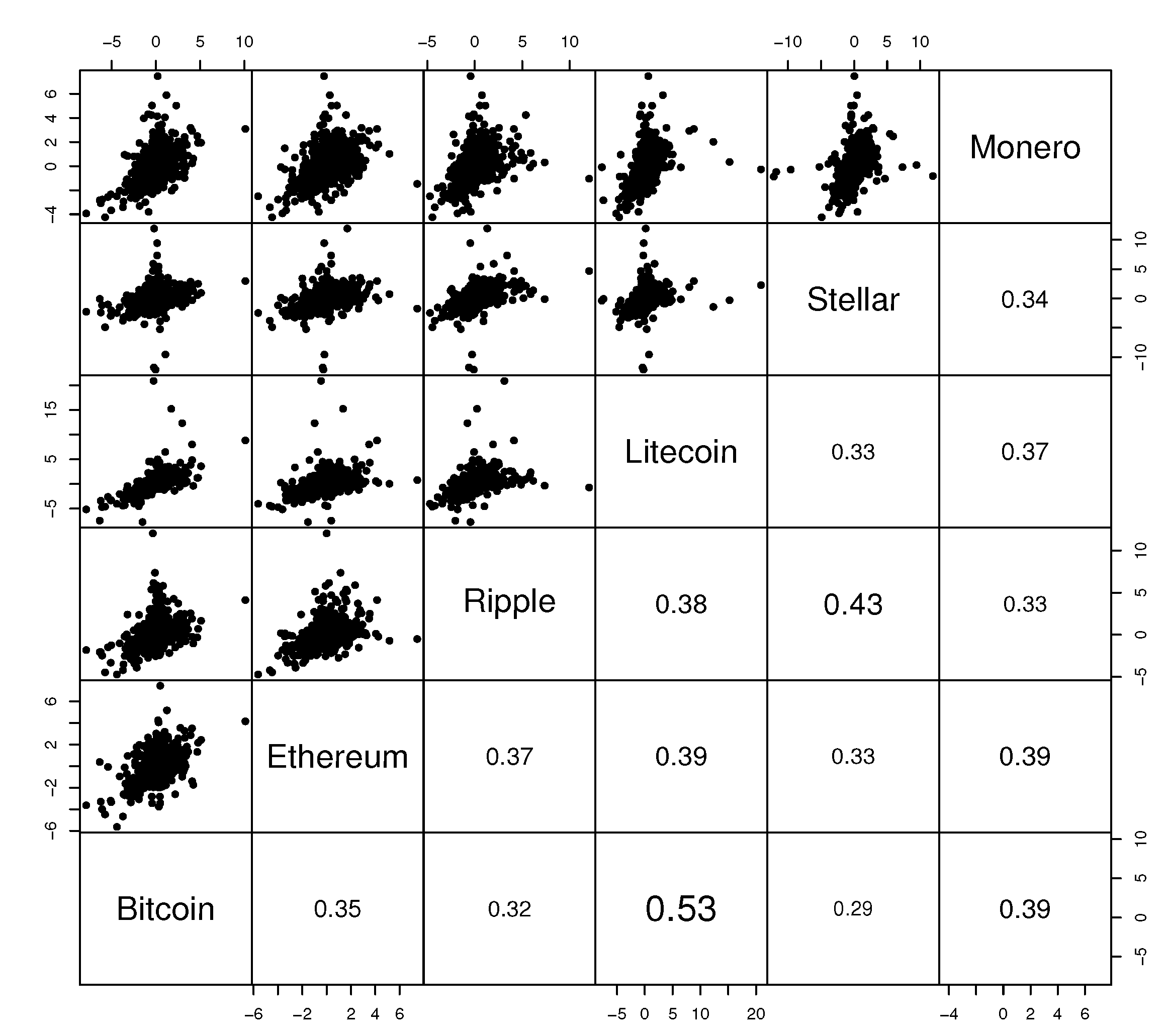
In this paper, to estimate the true dependence structure of the six crypto-currencies returns, we fit a Dvine pair-copula model to the independent standardized residuals from the GARCH fits specified in Table 3. Figure 4 shows the scatter plots of the standardized residuals on the upper-left panel (above diagonal). All pairs seem to be highly positively correlated. However, all plots show at least one extreme outlying point which has the potential to distort classical estimates of dependence measures. For example, Ripple shows a single outlier, much more extreme than the 99-quantile of the corresponding univariate distribution, which is not an extreme point in the BTC range. The effect of this atypical point may be observed, for example, on the Pearson $\rho$ which is 0.41, but without the single outlying observation it is 0.44. This suggests that a robust method should be applied to estimate the pair copulas.

We computed the two-step weighted maximum likelihood robust estimates proposed in Mendes et al. (2007). In the first step, outlying data points were identified by the Stahel–Donoho robust covariance estimator based on projections (Stahel 1981; Donoho 1982), and received zero weights. In the second step we computed the maximum likelihood estimates based on the reduced data. Computations were carried out on the free R platform.

Estimation followed the sequential approach (Aas et al. 2009; Aas and Berg 2009) where copula estimates from the previous tree were used to obtain the uniform (0,1) data in the current tree. Pairs composing Tree 1 were those showing stronger dependence, usually identified by either fitting a t-copula or computing some correlation coefficient. We ordered the variables in Tree 1 according to Kendall’s $\tau$ monotone correlation coefficient given in the bottom-right panel of Figure 4. The suggested order is: Monero–Bitcoin–Litecoin–Ethereum–Ripple–Stellar.

The best families for the 15 copulas composing the Dvine were defined based on an exhaustive search over all available families in the R package. The AIC and the BIC criteria were used for copula selection. The sequence found was: in Tree 1 all five bivariate copulas were from the BB7 family; the following seven copulas in trees 2 and 3 were t-copulas; the last three copulas in trees 4 and 5 were either t or Gaussian.

Table 4. Pair-copulas’ robust fits: copula family and estimates, dependence measures, the losses (gains) BB7-copula-based joint probability associated 1%-VaR in the upper row, and the $\pi$-copula-based risk under independence (bottom row).

Pairs in	Copula Family	Linear Coef $\mathit{\rho }$	Kendall’s $\mathit{\tau }$	Lower TDC ${\mathit{\lambda }}_{\mathit{L}}$	Upper TDC ${\mathit{\lambda }}_{\mathit{U}}$	Losses: BB7 Risk	Gains: BB7 Risk
Tree 1	(Parameters)	(Residuals Based)	(Copula Based)	(Copula Based)	(Copula Based)	Losses: ($\mathbf{\Pi }$ Risk)	Gains: ($\mathbf{\Pi }$ Risk)
(XMR,BTC)	BB7	0.523	0.601	0.746	0.566	0.745%	0.556%
	(1.923,2.361)					(0.01%)	(0.01%)
(BTC,LTC)	BB7	0.630	0.674	0.829	0.627	0.833%	0.635%
	(2.186,3.691)					(0.01%)	(0.01%)
(LTC,ETH)	BB7	0.462	0.616	0.751	0.565	0.783%	0.584%
	(1.918,2.632)					(0.01%)	(0.01%)
(ETH,XRP)	BB7	0.311	0.588	0.750	0.486	0.741%	0.492%
	(1.672,2.422)					(0.01%)	(0.01%)
(XRP,XLM)	BB7	0.236	0.608	0.740	0.605	0.746%	0.599%
	(2.083,2.301)					(0.01%)	(0.01%)

shows a summary of the results from the fits.

All BB7 copula estimates in Tree 1 imply a positive association; see the second column of Table 4. This was reflected o+in all copula based dependence measures, $\tau$, ${\lambda }_L$, and ${\lambda }_U$ (columns 4, 5, and 6). The Kendall’s $\tau$ coefficients had values around $0.6$ for all pairs in Tree 1, characterizing strong monotone dependence. On the other hand, the value of the linear correlation coefficient $\rho$ computed using the residuals, not being robust, suffered the influence of atypical points and may not have been the best statistic to inform about the dependence between the crypto-assets. For instance, $\rho$(XRP,XLM) is 0.24 much smaller than $\tau$(XRP,XLM) = 0.61.

The BB7 copula provided different lower and upper TDCs, discriminating the asymptotic dependence on the lower left and upper right corners. All TDC estimates are very large, meaning that at extreme scenarios one can expect a highly correlated market! For example, the conditional probability that Litecoin presents a loss greater than its VaR${}_{\alpha }$, given that Bitcoin has already shown returns larger than its VaR${}_{\alpha }$ is, as $\alpha$ goes to zero, 0.83 (also true the other way around).

Using simulations we computed the joint risk associated to pairs of the one-step-ahead VaR${}_{\alpha }$ values given in Table 3. As we can see in columns 7 and 8 of Table 4, the BB7 copula-based joint probability is much higher than under independence, equal to $0.01$% ($\mathrm{\Pi }$ copula). For example, the (univariate) 1%-VaR values of XMR and BTC reported in Table 3 have joint exceedance probability of 0.753% (joint losses) and 0.554% (joint gains). Note that as $\alpha$ goes to zero, the conditional probabilities (${\lambda }_L,{\lambda }_U$) for this pair are equal to (0.746, 0.566). The simulated copula values may be used to compute any other quantity of interest along with its standard errors.

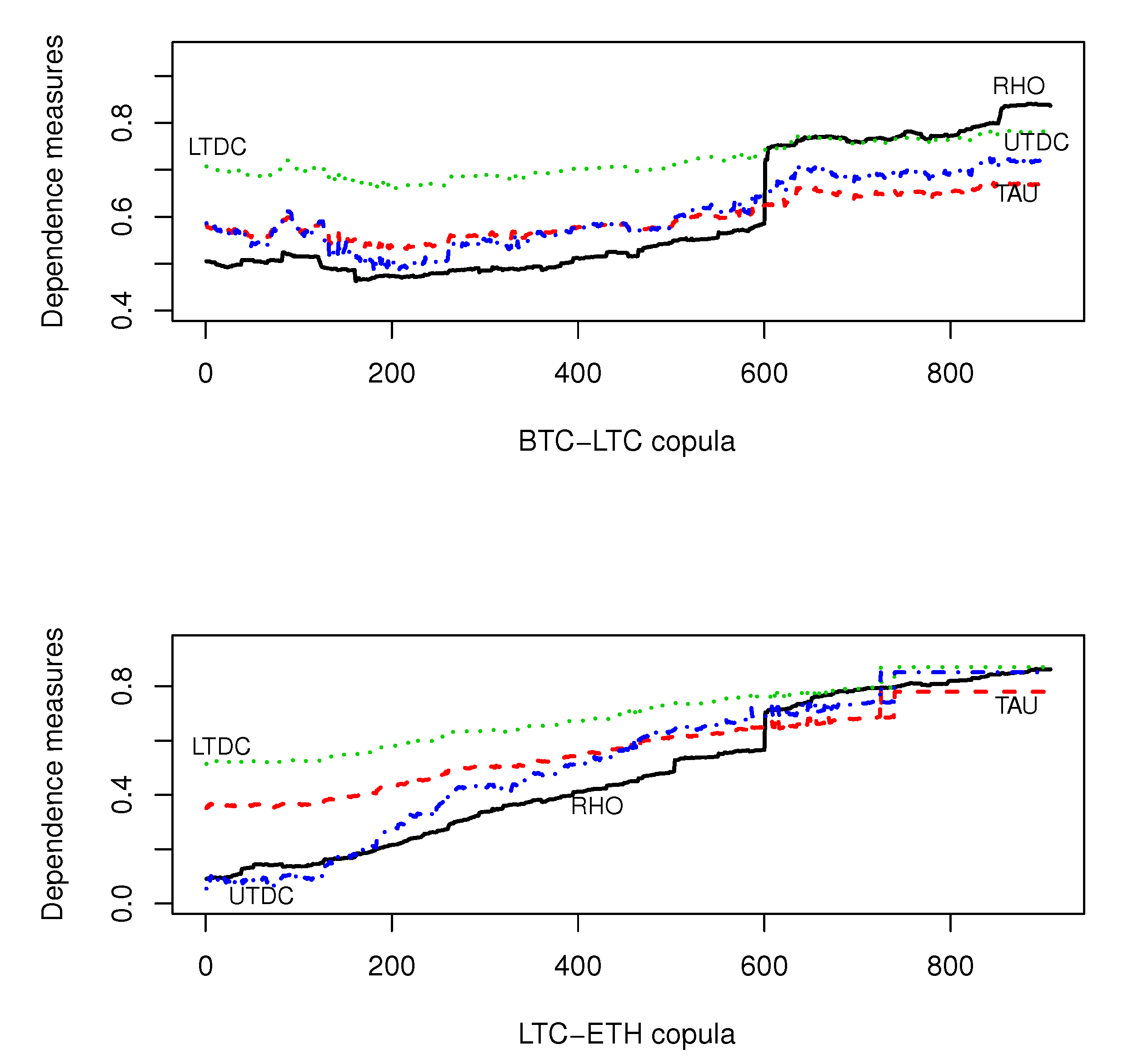
We applied the rolling window exercise to observe the behavior of the dependence measures along time. We fixed a initial window of size 730 days, and at each step the window was rolled 1 d ahead and the pair-copula model was fitted to the recent data. The resulting 907 dynamic estimates of the dependence measures were collected in Figure 5 where the results for the pairs (BTC, LTC) and (LTC, ETH) are depicted.

Many interesting things came out. First, it is clear that the strength of dependence among the crypto-assets has been increasing since 2015. The Pearson coefficient $\rho$, being non-robust and not well defined for our data, is the one showing the most dramatic behavior. For both pairs in Figure 5, the $\rho$ evolution shows a shift at the end of the first quarter of 2019. Actually, on 31 March 2019 Bitcoin initiated a 10-days lasting drawup, and on 2 April 2019 all six crypto-currencies presented simultaneous extreme gains with (BTC,LTC,ETH) returns achieving the values (16.06%, 23.08%, 14.91%), respectively. The effect of this three-dimensional extreme point is instantaneous on $\rho$, but it is slowly absorbed by the robust copula estimates. Note that these simultaneous extremes occurred during a stationary period of low volatility (see Figure 1) just preceding an exponential increase in prices. Just for the record, Euro returns were not extreme on this day.

In Table 4 we observed that ${\lambda }_L$ was higher than ${\lambda }_U$ for all pairs in Tree 1. The rolling window showed more than that. First, all three dependence coefficients—$\tau$, ${\lambda }_L$, and ${\lambda }_U$—showed an upward trend. However, the rate of increase of ${\lambda }_U$ was higher than ${\lambda }_L$. Thus, at the end of analyzed period the lower and upper TDC values were close, especially for the LTC-ETH copula. All this emphasizes that much care is needed when fitting models to large datasets, say, since the creation of Bitcoin, or including the first three or four years of the last decade. More reliable information certainly would come from models applied to recent data.

4.2. Dependence (by Cointegration)

To act simultaneously in several markets—including the virtual ones—global investors rely on their fast exchange of information and powerful computers. Their actions instantaneously feed and influence the whole market, reinforcing the simultaneous movements of financial time series. To assess series dynamic interdependencies one needs multivariate conditional models.

Data analysts often deal with non-stationary series such as interest rates, exchanges rates, spot and future prices, and so on. As we have seen in Section 2, all crypto-currencies prices ($P_t$) are I(1) unit root, non-stationary integrated of order 1. Multivariate regression models applied to price series will result in spurious correlations and inconsistent estimates. The corresponding first differences ($\Delta P_t$) were found to be I(0) stationary, and in this case a possible approach is to fit a vector autoregressive model (VAR). However, this model will still fail in the identification of relevant interdependencies if the series are cointegrated.

Whenever I(1) variables are cointegrated, there are subjacent economic forces constantly trying to restore some common long-run equilibrium relationship so that their deviations from equilibrium would not be permanent. A system composed by d I(1) variables is said to be cointegrated if there exists r I(0) stationary independent linear combinations of the d variables, $0<r<d$, the so called long-term equilibrium relationships. This error correction mechanism is incorporated into the VAR model resulting in the Vector Error Correction Model (VECM). The VECM$(p-1)$ model for the d crypto-currencies prices may be specified as:

$$\Delta {\mathbf{P}}_t=\mathbf{\Phi }{\mathbf{D}}_t+\mathbf{\Pi }{\mathbf{P}}_{t-1}+{\mathbf{\Gamma }}_1\Delta {\mathbf{P}}_{t-1}+\dots +{\mathbf{\Gamma }}_{p-1}\Delta {\mathbf{P}}_{t-p+1}+{\mathit{\epsilon }}_t$$

(3)

where ${\mathbf{D}}_t$ is a $(l\times 1)$ matrix of deterministic components such as constants, trends, seasonal dummies, etc, $\mathbf{\Phi }$ a parameter matrix, $\mathbf{\Pi }$ is the $(d\times d)$ long run impact matrix, $\mathbf{\Pi }={\mathbf{\Pi }}_1+\dots +{\mathbf{\Pi }}_p-{\mathbf{I}}_d$, ${\mathbf{\Pi }}_i$ are $(d\times d)$ matrices, ${\mathbf{\Gamma }}_k$ the short-run impact matrices, ${\mathbf{\Gamma }}_k=-{\sum }_{j=k+1}^p{\mathrm{\Pi }}_j,k=1,\dots ,p-1$, and ${\mathit{\epsilon }}_t$ a $(d\times 1)$ non-observable error vector, generated from a zero mean white noise process with constant covariance matrix. The term $\mathbf{\Pi }{\mathbf{P}}_{t-1}$ is I(0) and contains the cointegrating relations. $\Delta {\mathbf{P}}_t$ as well as its lagged values are I(0). Note the model may be further extended to include exogenous variables, or even allowing the original series $P_t$ to be integrated of order greater than 1.

In model (3) $\mathbf{\Pi }$ has reduced rank r and can be represented as a (not unique) multiplication of loading coefficients ${\mathit{\alpha }}_{(d\times r)}$ and cointegrating vectors ${\mathit{\beta }}_{(r\times d)}^{\prime }$. The components of $\mathit{\alpha }$ measure how fast the variables move back to their long-term relationship. Although the I(0) linear combinations ${\mathit{\beta }}^{\prime }{\mathbf{P}}_t$ are usually motivated by economic theories, in this paper we observe the market effect, how the system of most important crypto-currencies are linked together all sharing the same (or a few) common stochastic trend(s).

We started by performing a bivariate analysis investigating if Bitcoin is cointegrated with all other crypto-currencies plus Euro. We applied the Engle and Granger (1987) procedure and estimate the normalized $\beta$ by ordinary least squares, regressing Bitcoin on the other six series. All regression estimates were statistically significant and residuals were tested for stationarity applying the already described unit root tests. For all pairs except Euro, we were able to obtain I(0) residuals, so Bitcoin was not cointegrated with Euro but it was cointegrated with each one crypto-currency. The error correction model was then estimated considering the correct number of lags.

For all pairs in this analysis we found that the error correction mechanism is statistically significant but very slow. The estimates of the speed of adjustment parameters $({\alpha }_1,{\alpha }_2)$, given in

Table 5. Estimates of the speed of adjustment parameters $\alpha$ for all pairs. All estimates are 5% statistically significant.

Pairs	(BTC,ETH)	(BTC,RIP)	(BTC,LTC)	(BTC,XLM)	(BTC,XMR)
$\alpha$	(0.00502,0.00063)	(0.00453,0.000002)	(0.00528,0.00029)	(0.00477,0.000004)	(0.00573,0.00033)

, provide information about the amount of time necessary for the crypto-assets to return to their respective equilibrium values. Small values of $\alpha$ imply that it would take a long time for the variable to return to equilibrium. We observe that Bitcoin is faster than the other ones, and that its $\alpha$ values are close among all criptocoins. Roughly 0.5% of Bitcoin price deviations from its equilibrium are corrected in one day. Cointegration is really weak with Ripple and Stellar.

For the 6-dimensional crypto-assets data the Johansen trace and eigenvalue tests (Johansen 1988) indicated $r=2$; thus there were two cointegrating relations, and according to the AIC criterion $p=2$. Being cointegrated indicates that the already investigated runs of positive returns are not speculative; that is, prices do not exhibit explosive bubbles and move together, maintaining the equilibrium in the long run.

All coefficients in the model are statistically significant. In the rows of

Table 6. Estimates of the speed of adjustment parameters $\alpha$ for the six crypto-asset system. All estimates are 1% statistically significant.

	BTC	ETH	RIP	LTC	XLM	XMR
1st cointegrating vector	−0.13611	−0.03555	−0.00010	−0.00191	−0.00003	−0.00891
2nd cointegrating vector	−0.00251	−0.00037	−0.000002	−0.00003	−0.0000004	−0.00015

we give the two sets of $({\alpha }_1,\cdots ,{\alpha }_6)$ coefficients measuring the speed at which each crypto-asset is pulled back to equilibrium represented by the corresponding stationary portfolio. Now the contribution of Bitcoin and Ethereum is more evident, and it can be said that price information flows within the crypto-market although the speed of adjustment is still very slow implying that effects of a stochastic shock are very persistent.

In summary, the six analyzed crypto-coins are highly linearly and non-linearly correlated, increasing the possibility of significant joint falls in their values, which could lead to generalized margin calls. We note that Ciaian et al. (2016) have shown that Bitcoin prices are driven in the long run by investors speculative behavior, but it is not driven by macro-financial indicators.

5. Discussions

We have conducted a comprehensive statistical analysis of the top six crypto-currencies series, covering the period from 8 August 2015 to 31 January 2020, and representing approximately 77.4% of the total market capitalization at the time of writing. To assess the effects of the COVID-19 on the crypto-market, at the end of this section we add data from the first semester of 2020 and look for changes to what was discussed.

Using static and dynamic, univariate and multivariate, and simple and complex statistical approaches, we have confirmed most of the several findings scattered about the existing literature. They include the stylized facts: extremely large kurtosis (tail thickness), mean close to zero, non-normality, extreme points, almost nonexistent autocorrelation in returns (weak predictability), volatility clustering, high persistence, and long memory in the volatility. We also verified that, like real financial assets, crypto-currencies’ volatilities may be well captured by some GARCH models, which are able to provide accurate conditional risk measures. However, for the crypto-coins the tails of the GARCH conditional distribution are heavier than those found for stocks and exchange rates. Although all crypto-coins analyzed share these statistical features, Bitcoin (followed by Ethereum) seems to be more mature, with smaller risk measures, with statistics that are closer to those observed for other assets, and persistence close to those for real coins.

The existence of speculative bubbles in Bitcoin has been already tested (and rejected) in the literature. In this paper we confirmed that and made the link between speculative bubbles and episodes of runs of (consecutive) gains, the so-called drawups. We found that typically, for our series, the sum of consecutive gains was larger than the sum of consecutive losses. Even though the magnitudes of the Bitcoin drawdowns and drawups were smaller than those of other virtual coins, they were ten to twenty times greater than the values for Euro. The six crypto-currencies also presented some important episodes of joint drawups.

Our proposal for modeling the underlying return distribution—a semi-parametric mixture model, non-parametric for the bulk of the data, and an extreme value distribution (GPD) for each tail—showed an excellent adherence to the data, discriminated the left and right tails, and provided precise risk measures. We found that the right tail is riskier than the left tail for all series except for Bitcoin, which shows, in addition, smaller risk estimates. The unconditional risk measures based on a two-year rolling window sample performed even better.

It has been shown that crypto-coins are highly linearly and non-linearly correlated. Our pair-copula model uncovered new features: At extreme scenarios one can expect a highly correlated market, with extreme joint gains behaving differently from large joint losses. Simultaneous extremes may occur during periods of low volatility. All crypto-coins are positively correlated, and the strength of dependence has been increasing since 2015. However, the linear correlation coefficient $\rho$ may not be the best statistic to inform one about the dependence between the crypto-assets.

Prices are linked together forming a cointegrated system with two cointegrating relations driven by crypto-market forces. Price information flows within the crypto-market, although the speed of adjustment to the long run equilibrium is very slow, implying that effects of a stochastic shock may last for a long time. Bitcoin is not cointegrated with Euro but it is cointegrated with each one crypto-currency.

Our data ended by the time of the onset of COVID-19 pandemic, and right now we do not know their effects on the economy, on people new habits, on stock- and crypto-markets, and so on, even though we can already see some advances in technology. To provide some insights on what may be just around the corner for the crypto-market, we add to the analysis the first semester of 2020.

We basically compared the second semester of 2019 with the first semester of 2020. The first thing that came to our attention is that all crypto-coins prices showed an upward trend during the first two months of 2020, after a dramatic loss in value during the whole second semester of 2019; see Figure 6. However, on 12 March 2020, all crypto-coins prices fell about 61%, reaching a point that could be expected based of the previous 6-months’ downhill trend of price levels. In other words, the two initial months of January and February of 2020 could have been a speculative bubble. We carried out the dependence test of McQueen and Thorley (1994) and found that Bitcoin and Stellar indeed accepted the null of a speculative bubble, whereas for all others crypto-currencies the test was inconclusive.

After the joint extreme fall of March 2020, all prices seemed to randomly walk around a new level, lower than those attained in 2017. It is interesting to observe that, in spite of the March outlying negative return, the accumulated return in the first semester of 2020 is positive for all crypto-currencies except XRP, whereas it was negative and significant in 2019/2 and for all crypto-assets. For example, for Bitcoin and Ethereum the cumulative one-semester returns was, respectively, 27.4% and 74.7% in 2020/1, and $-32.4$% and $-56.1$% in 2019/2.

The extreme negative return has a large influence on the 2020 returns’ basic statistics. For all crypto-coins we observed a more extreme minimum, higher standard deviations, larger skewness coefficients, and specially very large kurtosis. All 2020 sample means, although negative, are still statistically zero.

Interesting results came out when we incorporated the 2020/1 data in the kurtosis rolling window analysis of Section 3.1. When the 12 March 2020 Bitcoin extreme negative outlier of −48.69% entered in the calculating window, the kurtosis value jumped from approximately 4 to 44.8 and remained huge during the whole first semester of 2020. However, without this single extreme point, the kurtosis values stayed around the 2.7 level for the COVID-19 period. Similar behavior was observed for Ethereum, which presented a kurtosis value of 42.20 after the 12 March 2020 outlier of −56.27 was entered in the computations. Without this extreme observation the Ethereum kurtosis values stayed close to the Euro mean level during all 2020/1. In spite of this striking result, from a practical conservative viewpoint, the risk- or portfolio-manager/investor may find ut safer to consider the kurtosis values inflated by a single outlying point as inputs in her/his models. Alternatively, he/she may use a larger window for long run investments.

Finally, we carried out the rolling window exercise to assess changes in the dynamic copula-based dependence measures. Based on a one-semester window length, we observed estimates close to the values observed at the end of 2019, which stayed almost constant during the six-months of the COVID-19 pandemic. It was also noted that all rolling-window-based basic statistics seemed to stabilize during the second quarter of 2020, as if staying on hold. We wonder if this may be related to the crypto-market player’s profile, that is, to the common degree of risk aversion, level of wealth, level of information, and so on, which together make them investors looking for alternative long run investments and for whom liquidity might not be an issue.

The crypto-market is still in its infancy, but it is growing up rapidly, with leading crypto-currencies already showing numbers close to those of real coins/assets traded in mature markets. As such, the crypto-assets are also becoming interesting alternative investments for frequent traders, who though, should keep in mind that more reliable statistical conclusions would come from models applied to recent data.