Cryptocurrency Trading Using Machine Learning

Abstract

We present a model for active trading based on reinforcement machine learning and apply this to five major cryptocurrencies in circulation. In relation to a buy-and-hold approach, we demonstrate how this model yields enhanced risk-adjusted returns and serves to reduce downside risk. These findings hold when accounting for actual transaction costs. We conclude that real-world portfolio management application of the model is viable, yet, performance can vary based on how it is calibrated in test samples.

1. Introduction

Is active trading viable in cryptocurrency markets and can it yield superior performance relative to a buy-and-hold approach? Using a direct reinforcement (DR) model we demonstrate that, yes, active trading is both viable and profitable in such markets and can yield superior risk-adjusted performance relative to a passive buy-and-hold approach. We show that despite the high volatility risks which cryptocurrency traders face, our DR approach can serve to actively reduce downside risks in their portfolios.

The motivation for our DR model stems from two streams of literature. The first is the growing interest in explaining or forecasting the price behavior of cryptocurrencies and the formation of trading strategies in such markets (Akcora et al. 2018; Baur and Dimpfl 2018; Brauneis and Mestel 2018; Catania et al. 2019; Phillip et al. 2018). This stream of literature shows how these blockchain-based digital assets have distinct technological and network attributes that set them apart from traditional assets. In addition, this stream of literature also demonstrates the growing need in understanding whether active trading in such markets is viable. For example, Tzouvanas et al. (2020) show momentum trading may be profitable but only in the short-run, while Grobys and Sapkota (2019) provide evidence that momentum trading is not profitable when examining a large cross-section of cryptocurrencies. Makarov and Schoar (2020) maintain “…while significant attention has been paid to the dramatic ups and downs in the volume and price of cryptocurrencies, there has not been a systematic analysis of the trading and efficiency of cryptocurrency markets…” (p. 1). In addition to this, and as is shown in Koutmos and Payne (2020), there are many heterogeneous traders present in bitcoin exchanges that carry different expectations about the future direction and volatility of bitcoin. Thus, there are many challenges associated with trying to model bitcoin prices accurately and determining optimal trading strategies. Our DR approach overcomes such obstacles specifically since it is eliminates the need to search for and select explanatory factors for cryptocurrencies or to account for the trading behavior of different types of investors. This strength in our approach is further important especially considering how cryptocurrency prices can undergo regime shifts across time (Koutmos 2018; Li and Wang 2017).

The second stream of literature that motivates our DR model is the growing interest in machine learning methods in economic applications or the development of trading systems that can be automated (Acosta 2018; Henrique et al. 2019; Saltzman and Yung 2018). In fact, there are a growing number of patents and patent filings that devise machine learning methods for either stock selection or trading automation Kumar and Raychaudhuri (2014). Nevertheless, Huck (2019) indicates that, first, machine learning approaches can yield mixed results depending on the number of predictor variables and, second, may not provide a competitive edge for investors given how readily available these models now are to all investors in the market. Notwithstanding their limitations, there is a budding strand of recent literature that tests the ability of machine learning methods to be used effectively in portfolio allocation decisions, exchange rate forecasting and even bankruptcy prediction (Jiang et al. 2020; Kristóf and Virág 2020; Zhang and Hamori 2020). Given the increasing use of cryptocurrencies by financial institutions and the investment public, it is important to test whether such methods can also be applied profitably or used for risk management purposes across cryptocurrency exchanges. As mentioned by Koutmos (2019), using macroeconomic variables and models that successfully explain the price variations in traditional asset classes may not be effective in modeling cryptocurrency price changes.

As is discussed further, and apart from the enhanced performance it yields relative to a buy-and-hold approach, our DR model is advantageous for the following reasons. First, it eliminates the need to build a forecasting model for price movements. This is important because this avoids Bellman’s curse of dimensionality and the need to somehow aggregate high dimensional data into a parsimonious model. Second, it uses an adaptive algorithm that learns trading strategies which balance returns while avoiding a specified measure of risk.

The remainder of our study proceeds as follows. Section 2 describes our DR model. Section 3 discusses our cryptocurrency sample data. Section 4 presents results from experimental trials of our model. In this section, we show how our DR model provides superior risk-adjusted performance relative to a buy-and-hold strategy. Finally, Section 5 concludes and makes suggestions for future extensions of our analysis.

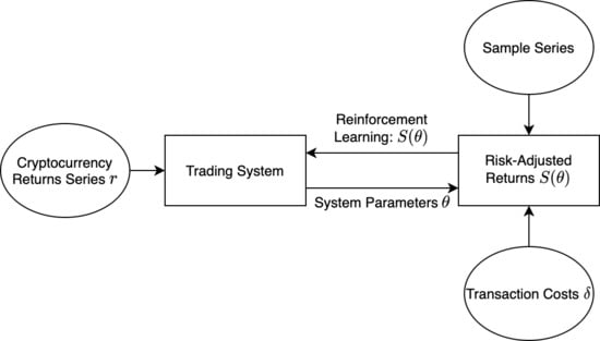
2. Direct Reinforcement Learning

A trading system’s ultimate objective is to optimize some measure of risk-adjusted returns across time while also considering transaction costs. As in Moody and Saffell (2001), our direct reinforcement (DR) approach contrasts with methods such as dynamic programming, temporal difference learning or q-learning.1 Such models seek to learn a value function and lend themselves to problems (such as checkers, backgammon or tic-tac-toe) where immediate performance feedback is not promptly available at each time interval. On the other hand, and since trading decisions are readily measurable at each time interval, our DR model can learn to optimize risk-adjusted returns because it is receiving feedback at each time interval (each trading day in our case here).

See (Bellman 1957; Sutton 1988; Watkins and Dayan 1992). Direct reinforcement learning, or, recurrent reinforcement learning, as it is often synonymously referred to, indicates a class of models that do not have to learn a value function Carapuço et al. (2018).

In our DR model, we seek to estimate the parameters of a nonlinear autoregressive model that achieve the greatest risk-adjusted returns. Our trader can take long or short positions in each of the cryptocurrency markets that we sample, $F_t\in \{1,-1\}$, and at each time interval t.2 $F_t$ values of 1 and $-1$ correspond to an entirely long and short position respectively. The cryptocurrency price series being traded is denoted as $z_t$. The position, $F_t$, is established or maintained at the end of time interval t and re-evaluated at the end of $t+1$. While trading is possible at each time interval, transaction fees discourage excessive trading.3

The traded cryptocurrency price series is denoted as $z_t$ and returns are $r_t=z_t/z_{t-1}-1$. $F_t$ can be represented as a function of (learned) system parameters $\theta$:

$$F_t=\mathrm{sign}({\theta }_0+{\theta }_1{F}_{t-1}+{\theta }_2{r}_t+{\theta }_3{r}_{t-1}+\dots +{\theta }_{m+1}{r}_{t-m+1})$$

(1)

whereby m is the number of autoregressive returns to be used. In this way, the model “decides” its next position based on the last m returns of the asset. During training, the discreet sign function is replaced with the differentiable tanh function, in which partial positions can be held for values $-1<F_t<1$. Trading returns $R_t$ can then be defined as:

$$R_t=(1+F_{t-1}{r}_t)(1-\delta |F_t-F_{t-1}\left|\right)$$

(2)

with $\delta$ as the transaction cost. The performance measure we use to provide feedback to (1) and (2) is the Sortino ratio:

$$\mathrm{Sortino}=\frac{\mathrm{mean}\left(R\right)}{\sqrt{\mathrm{mean}(min{(R,0)}^2)}}$$

(3)

As Moody and Saffell (2001) indicate, several measures and variations thereof can be used to provide performance feedback. In untabulated results (available on request), we show that the Sharpe ratio discourages the model from making trades that produce large positive returns. This is because large positive returns have a symmetric impact on volatility as do large negative returns of equal magnitude (and volatility ‘penalizes’ the Sharpe ratio, regardless of the sign of returns).4

The Sortino ratio in (3) is thus chosen to be the reward function S, whereby parameters $\theta$ can be optimized via gradient ascent for each epoch:

$$\Delta \theta =\eta \frac{dS\left(\theta \right)}{d\theta }$$

(4)

where $\eta$ is the learning rate. This is repeated until convergence, whereby the derivative $\frac{dS\left(\theta \right)}{d\theta }$ is calculated with a dynamic computational graph using PyTorch Paszke et al. (2017). After optimal parameters are found over a training set, simulated trading results are created from the next time intervals, as we discuss further in Section 4. The full training process is detailed in Appendix A.

3. Data Sample

We test our DR model using five of the largest cryptocurrencies in circulation (bitcoin, ethereum, litecoin, ripple and monero, respectively). Our sample range is from 26 August 2015 to 12 August 2019 (1447 data points) for all cryptocurrencies (some cryptocurrencies, such as bitcoin, are relatively more established while others, such as ethereum, started in August of 2015).

Presently, bitcoin by itself constitutes over 65% of the total market capitalization of all cryptocurrencies in circulation. Together, our five sampled cryptocurrencies account for about 80% of the present total market capitalization. Likewise, these five presently account for more than 50% of the total trade volume of all cryptocurrencies in circulation.

Table 1. Sampled Cryptocurrencies

Cryptocurrency	Abbrev.	Avg. Price	Max	Min.	Avg. Volume	Avg. Mkt. Cap
Bitcoin	BTC	$4057.42	$19,497.40	$210.49	$4,450,445,943	$69,165,755,657
Ethereum	ETH	$207.28	$1396.42	$0.43	$1,739,231,393	$20,456,600,907
Litecoin	LTC	$51.82	$358.34	$2.63	$613,577,135	$2,933,407,200
Ripple	XRP	$0.27	$3.38	$0.0041	$456,691,482	$10,744,494,433
Monero	XMR	$72.27	$469.20	$0.36	$39,390,717	$1,147,314,395

This table shows the sampled cryptocurrencies in our data sample (our sample range is from 26 August 2015 to 12 August 2019). For this sample range, we show the average, maximum and minimum market prices, respectively, average daily trading volume and, finally, average market capitalization. The data is sourced from coinmarketcap.com.

shows summary statistics for our sampled cryptocurrencies. Altogether, the average daily trade volume over our sample period exceeded $7 billion. In relation to asset classes investors are more familiar with (such as equities, real estate, and bonds), cryptocurrencies display high levels of price volatility. For example, and for our sample period, bitcoin had a low price of $210 and a high price of $19,000.

4. Discussion of Findings

Following Moody and Saffell (2001), the trading system is trained for the first 1000 days, and simulated trading signals for the following 100 days are produced using the learned parameters. The training window is then shifted to include this tested-on data, and model is retrained and tested on the following 100 days.5 In this way, trading data is completely out-of-sample. This process is repeated until trading signals are obtained for the whole 447-day test window, using independent models for each cryptocurrency.

Table 2. Portfolio Performance Metrics.

Cryptocurrency	Cum. Returns		Sharpe		Sortino		Max Drawdown		Value-at-Risk
	BH	DR	BH	DR	BH	DR	BH	DR	BH	DR
Bitcoin	1.352	3.398	0.037	0.094	0.053	0.143	0.616	0.434	0.059	0.056
Ethereum	0.302	0.240	−0.031	−0.041	−0.042	−0.056	0.870	0.823	0.081	0.082
Litecoin	0.637	0.837	0.005	0.017	0.008	0.027	0.818	0.767	0.083	0.083
Ripple	0.441	0.783	−0.012	0.013	−0.020	0.022	0.611	0.591	0.083	0.082
Monero	0.459	1.374	−0.010	0.039	−0.014	0.057	0.780	0.796	0.082	0.079

This table shows performance metrics between a buy-and-hold (BH) approach and our direct reinforcement (DR) model. For each performance metric (cumulative returns, Sharpe ratio, Sortino ratio, maximum drawdown and value-at-risk, respectively), we highlight in bold the metric that enhances the portfolio for our out-of-sample test period. Cumulative returns are expressed in decimal form (e.g., 1.352 corresponds to 135%). Value-at-risk is also expressed in decimal form (e.g., 0.059 corresponds to 5.9%).

shows portfolio metrics of our DR model in relation to a buy-and-hold approach. In terms of cumulative returns and risk-adjusted returns (as shown by the Sharpe and Sortino ratios), we see that our DR model outperforms a buy-and-hold approach for all the sampled cryptocurrencies with the exception of ethereum. Our DR performs especially well with bitcoin where, as we show in Figure 1, it more than triples the value of 1 bitcoin.

In terms of reducing risk (as measured by maximum drawdown and value-at-risk), our DR model outperforms buy-and-hold in all cases except for monero (when measured using maximum drawdown) and ethereum (when measured using value-at-risk, although by a negligible amount).

Our experimental results reported in Table 2 and Figure 1 account for transaction fees of 0.10% (see Footnote 3), which are applied when a trade is initiated.

5. Conclusions

We show how reinforcement machine learning can make cryptocurrency trading decisions that optimize actively managed portfolios. Our results compare favorably to a naive buy-and-hold approach. Theoretically, these results provide some preliminary evidence that cryptocurrency prices may not follow a purely random walk process. This is because we show how our active trading strategy can yield superior risk-adjusted returns for investors and even reduce portfolio downside risk across time and if the model is trained adequately. Thus, the possibility of devising novel active trading strategies in the future, based on some quantitative or theoretical framework, may be useful in cryptocurrency markets instead of relying on naive buy-and-hold approaches. Our findings also agree theoretically with Lahmiri and Bekiros (2019), who show that cryptocurrency prices may not follow a random walk process. Chen and Hafner (2019) also report weak evidence that cryptocurrencies follow random walks consistently across time. Instead, their prices appear to be driven by sentiment. From a practical perspective, our application of the direct reinforcement methodology we describe can be replicated and tested across a range of cryptocurrencies or other traditional assets such as equities or index funds. Finally, it is important to emphasize that our approach can be successfully applied in markets where both buying and shorting are possible.

In light of these favorable findings, however, we echo the sentiments of Gold (2003) regarding finding optimal parameters in a machine learning model: “…optimal values in one market may be sub-optimal for another…” (p. 368). This claim especially highlights some of the challenges with integrating machine learning for economic decision-making. Namely, machine learning takes an atheoretical ‘black box’ approach. Nonetheless, machine learning poses countless opportunities.

With regards to our DR approach, it remains unsaid whether integrating microstructure variables (such as number of cryptocurrency users or trading activity) in addition to returns can yield superior degrees of portfolio performance across a larger subset of cryptocurrencies and across market regimes.

References

1. Acosta, Marco A. 2018. Machine learning core inflation. Economics Letters 169: 47–50. [Google Scholar] [CrossRef]
2. Akcora, Cuneyt Gurcan, Matthew F. Dixon, Yulia R. Gel, and Murat Kantarcioglu. 2018. Bitcoin risk modeling with blockchain graphs. Economics Letters 173: 138–42. [Google Scholar] [CrossRef] [Green Version]
3. Baur, Dirk G., and Thomas Dimpfl. 2018. Asymmetric volatility in cryptocurrencies. Economics Letters 173: 148–51. [Google Scholar] [CrossRef]
4. Bellman, Richard. 1957. Dynamic Programming. Princeton: Princeton University Press. [Google Scholar]
5. Brauneis, Alexander, and Roland Mestel. 2018. Price discovery of cryptocurrencies: Bitcoin and beyond. Economics Letters 165: 58–61. [Google Scholar] [CrossRef]
6. Carapuço, João, Rui Neves, and Nuno Horta. 2018. Reinforcement learning applied to forex trading. Applied Soft Computing 73: 783–94. [Google Scholar] [CrossRef]
7. Catania, Leopoldo, Stefano Grassi, and Francesco Ravazzolo. 2019. Forecasting cryptocurrencies under model and parameter instability. International Journal of Forecasting 35: 485–501. [Google Scholar] [CrossRef]
8. Chen, Cathy Yi-Hsuan, and Christian M. Hafner. 2019. Sentiment-induced bubbles in the cryptocurrency market. Journal of Risk and Financial Management 12: 53. [Google Scholar] [CrossRef] [Green Version]
9. Gold, Carl. 2003. Fx trading via recurrent reinforcement learning. Paper presented at 2003 IEEE International Conference on Computational Intelligence for Financial Engineering, Hong Kong, China, March 20–23; pp. 363–70. [Google Scholar]
10. Grobys, Klaus, and Niranjan Sapkota. 2019. Cryptocurrencies and momentum. Economics Letters 180: 6–10. [Google Scholar] [CrossRef]
11. Henrique, Bruno Miranda, Vinicius Amorim Sobreiro, and Herbert Kimura. 2019. Literature review: Machine learning techniques applied to financial market prediction. Expert Systems with Applications 124: 226–51. [Google Scholar] [CrossRef]
12. Huck, Nicolas. 2019. Large data sets and machine learning: Applications to statistical arbitrage. European Journal of Operational Research 278: 330–42. [Google Scholar] [CrossRef]
13. Jiang, Zhenlong, Ran Ji, and Kuo-Chu Chang. 2020. A machine learning integrated portfolio rebalance framework with risk-aversion adjustment. Journal of Risk and Financial Management 13: 155. [Google Scholar] [CrossRef]
14. Koutmos, Dimitrios. 2018. Liquidity uncertainty and bitcoin’s market microstructure. Economics Letters 172: 97–101. [Google Scholar] [CrossRef]
15. Koutmos, Dimitrios. 2019. Market risk and bitcoin returns. Annals of Operations Research, 1–25. [Google Scholar] [CrossRef]
16. Koutmos, Dimitrios, and James E. Payne. 2020. Intertemporal asset pricing with bitcoin. Review of Quantitative Finance and Accounting, 1–27. [Google Scholar] [CrossRef]
17. Kristóf, Tamás, and Miklós Virág. 2020. A comprehensive review of corporate bankruptcy prediction in hungary. Journal of Risk and Financial Management 13: 35. [Google Scholar] [CrossRef] [Green Version]
18. Kumar, Piyush, and Rajat Raychaudhuri. 2014. Stock Ranking Predictions Based on Neighborhood Model. U.S. Patent Application No. 13/865,676, March 4. [Google Scholar]
19. Lahmiri, Salim, and Stelios Bekiros. 2019. Cryptocurrency forecasting with deep learning chaotic neural networks. Chaos, Solitons & Fractals 118: 35–40. [Google Scholar]
20. Li, Xin, and Chong Alex Wang. 2017. The technology and economic determinants of cryptocurrency exchange rates: The case of bitcoin. Decision Support Systems 95: 49–60. [Google Scholar] [CrossRef]
21. Makarov, Igor, and Antoinette Schoar. 2020. Trading and arbitrage in cryptocurrency markets. Journal of Financial Economics 135: 293–319. [Google Scholar] [CrossRef] [Green Version]
22. Markovitz, Harry M. 1959. Portfolio Selection: Efficient Diversification of Investments. Hoboken: John Wiley. [Google Scholar]
23. Moody, John, and Matthew Saffell. 2001. Learning to trade via direct reinforcement. IEEE Transactions on Neural Networks 12: 875–89. [Google Scholar] [CrossRef] [Green Version]
24. Paszke, Adam, Sam Gross, Soumith Chintala, Gregory Chanan, Edward Yang, Zachary DeVito, Zeming Lin, Alban Desmaison, Luca Antiga, and Adam Lerer. 2017. Automatic differentiation in PyTorch. Advances in Neural Information Processing Systems 32: 8024–35. [Google Scholar]
25. Phillip, Andrew, Jennifer S. K. Chan, and Shelton Peiris. 2018. A new look at cryptocurrencies. Economics Letters 163: 6–9. [Google Scholar] [CrossRef]
26. Saltzman, Bennett, and Julieta Yung. 2018. A machine learning approach to identifying different types of uncertainty. Economics Letters 171: 58–62. [Google Scholar] [CrossRef]
27. Sutton, Richard S. 1988. Learning to predict by the methods of temporal differences. Machine Learning 3: 9–44. [Google Scholar] [CrossRef]
28. Tzouvanas, Panagiotis, Renatas Kizys, and Bayasgalan Tsend-Ayush. 2020. Momentum trading in cryptocurrencies: Short-term returns and diversification benefits. Economics Letters 191: 108728. [Google Scholar] [CrossRef]
29. Watkins, Christopher J. C. H., and Peter Dayan. 1992. Q-learning. Machine Learning 8: 279–92. [Google Scholar] [CrossRef]
30. Zhang, Yuchen, and Shigeyuki Hamori. 2020. The predictability of the exchange rate when combining machine learning and fundamental models. Journal of Risk and Financial Management 13: 48. [Google Scholar] [CrossRef] [Green Version]