Article

Long Memory in the Volatility of Selected Cryptocurrencies: Bitcoin, Ethereum and Ripple

1
Department of Business Informatics, Faculty of Business Administration, Marmara University, Istanbul 34722, Turkey
2
Department of Capital markets, School of Banking & Insurance, Marmara University, Istanbul 34722, Turkey
3
Department of Insurance, School of Banking & Insurance, Marmara University, Istanbul 34722, Turkey
4
Peter F. Drucker and Masatoshi Ito Graduate School of Management, Claremont Graduate University, Claremont, CA 91711, USA
*
Author to whom correspondence should be addressed.
J. Risk Financial Manag. 2020, 13(6), 107; https://doi.org/10.3390/jrfm13060107
Submission received: 6 March 2020 / Revised: 26 May 2020 / Accepted: 27 May 2020 / Published: 29 May 2020

Abstract

:
This paper examines the volatility of cryptocurrencies, with particular attention to their potential long memory properties. Using daily data for the three major cryptocurrencies, namely Ripple, Ethereum, and Bitcoin, we test for the long memory property using, Rescaled Range Statistics (R/S), Gaussian Semi Parametric (GSP) and the Geweke and Porter-Hudak (GPH) Model Method. Our findings show that squared returns of three cryptocurrencies have a significant long memory, supporting the use of fractional Generalized Auto Regressive Conditional Heteroscedasticity (GARCH) extensions as suitable modelling technique. Our findings indicate that the Hyperbolic GARCH (HYGARCH) model appears to be the best fitted model for Bitcoin. On the other hand, the Fractional Integrated GARCH (FIGARCH) model with skewed student distribution produces better estimations for Ethereum. Finally, FIGARCH model with student distribution appears to give a good fit for Ripple return. Based on Kupieck’s tests for Value at Risk (VaR) back-testing and expected shortfalls we can conclude that our models perform correctly in most of the cases for both the negative and positive returns.

1. Introduction

Since the early 2000s, the perception of investors about traditional financial markets, their systems and policies has changed dramatically. There is a global loss of confidence in the central bank based, fiat currency centered, interconnected financial system. There are many reasons for this shift in confidence. First of all, loose monetary policies of central banks and the simultaneous global imbalances created an asset price bubble in early 2000s, which led to the global financial crisis in 2008 and the resulting Great Recession (Allen and Carletti 2010; Carmassi et al. 2009). Financial crises are like storms for economies: they increase unemployment rates and financing costs, deepen recessions, and negatively affect global trade. Economies, especially emerging economies, need increasingly more financing in order to refinance their debts in an environment of increasing risk premiums (Dominguez et al. 2012).
The 2008 financial crisis, at the same time, increased the volatility and thus changed the risk perception of investors in global financial markets. Therefore, many investors trading in financial markets, especially those invested in markets which did not fair the storm well, lost their confidence in the ability of central banks to manage financial crises (Bordo and Siklos 2017; Cukierman 2013; Wagner 2010).
Simultaneously, during this period since 2000, many countries have tried to use currency depreciations via lower interest rates as a competitive tool in global trade. These currency wars between the major central banks have contributed to the excessive asset price increases during the early part of the century. On the other hand, these currency manipulations have negatively impacted investors’ confidence in financial markets, their regulators and central banks and the overall global financial system (Blanchard 2016; Caballero et al. 2015; Cline and Williamson 2010).
The policy uncertainty, market volatility and change in investor confidence in the financial system, coupled with recent developments in blockchain technology has led to the invent of, and (very quickly) increasing demand for, cryptocurrencies (Çağlar 2007; Liu and Tsyvinski 2018; Panagiotidis et al. 2018, 2019, 2020).
Since its initial introduction, Bitcoin—the first and most common cryptocurrency—has received unexpected attention and even notoriety in financial markets and has become part of commonplace financial metrics to be followed by investors. According to Hileman and Rauchs (2017), the rise of cryptocurrencies in financial markets can be attributed to the fact that unlike traditional fiat currencies, cryptocurrencies are fully digital assets; have fast, reliable, low cost and anonymous exchange systems; and are not controlled by a central authority such as central banks.
Barber et al. (2012) explored the Bitcoin as a potential solution to the structural problems in financial systems. While examining the advantages of Bitcoin over other cryptographic currencies, they conclude that Bitcoin has the potential to be a long-term stable currency. They state that, if the system design is properly supported, decentralized digital currencies can have a strong influence on financial markets (Barber et al. 2012).
In the last decade, the increasing popularity of cryptocurrencies has resulted in many to be created. By the year 2018, there were approximately 1700 different cryptocurrencies in existence with a total global daily transaction volume of 11 billion US dollars (Hileman and Rauchs 2017). Yet, three major cryptocurrencies make up 60% of the transaction volume and 86% of the total cryptocurrency market capitalization: namely Bitcoin, Ethereum and Ripple (BitInfoCharts 2018).
This fast development and increasing spread of cryptocurrencies evidenced by their increasing transaction volume and market capitalization, has identified cryptocurrencies as a major disruptive instrument in international financial markets. Thus, the academic and practitioner debate of how to classify a cryptocurrency in the world of investments, namely whether as a “security,” a “commodity,” or a “currency”, has become more significant and heated over the years. This classification is important in many aspects of the study of these instruments, especially in determining the role cryptocurrencies will play in diversified portfolios of rational investors (Jackson 2018). The debate on this issue is still ongoing both in academic and practitioner worlds.
Cryptocurrency valuations, especially that of Bitcoin, have increased excessively against the dollar in the last decade. As a result, they have become an attractive investment option to many investors. An increasing number of investors now include, or consider including, cryptocurrencies in their portfolio selection processes. Even though the traditional risk-return trade-off establishes the positive correlation between risk and return, investors, when making portfolio decisions, tend to overestimate the potential returns of an asset, while often ignoring or underestimating the risk.
There are two major risks that cryptocurrency investors are exposed to. First of all, the cryptocurrencies do not have intrinsic asset values due to their blockchain based structures. Second, cryptocurrency returns have significantly higher volatility than the returns of more traditional financial assets such as stocks or precious metals etc. (Bouri et al. 2019; Liu and Tsyvinski 2018). Similarly, cryptocurrency returns have been shown to have significantly higher volatility than major world fiat currencies (Caginalp and Caginalp 2018; Catania et al. 2018; Sahoo 2017).
Since volatility of investment returns is a fundamental issue for the smart investor and portfolio manager in contemporary financial markets, adequate modeling for volatility of cryptocurrencies becomes vital for risk management. In this study, we model the volatility of cryptocurrencies by appropriate Generalized Auto Regressive Conditional Heteroscedasticity (GARCH) type models. Unlike similar studies in the literature, the scope of the research is not limited to Bitcoin only, but includes all three largest market capitalization cryptocurrencies: Bitcoin, Ethereum and Ripple.
Bitcoin and Ethereum are decentralized digital currencies without a single administrator and operate on public blockchain ledgers. Unlike the other two, Ripple, is a centralized cryptocurrency, which operates on a distributed ledger controlled by the Ripple Labs. In other words, all the ledger books on which Ripple cryptocurrency (XRP) is traded, are managed by the Ripple Labs itself. Whereas Bitcoin and Ethereum are released and added to the network as they are mined by independent sources, Ripple Labs releases a certain amount of Ripple cryptocurrency tokens each month. In addition, unlike its other cryptocurrency counterparts, Ripple cryptocurrency is intentionally designed to be an effective tool in international fiat money transfers. Even with their slight differences in structure, these three cryptocurrencies make up most of the market capitalization and more than half the world trading volume. Therefore, correctly modelling their volatilities is a very important contribution to the literature.
On the other hand, literature using persistency analysis on cryptocurrencies is continuously growing. Specifically, the increasing evidence of long-term dependence in cryptocurrency markets provides evidence that cryptocurrency price changes are not random and future prices of cryptocurrencies are predictable. This predictability in prices contradicts with the efficient markets hypothesis and random walk expectations of Malkiel and Fama (1970). If cryptocurrency prices exhibit long memory, investors can predict future prices and beat the market (Mensi et al. 2019). Therefore, the presence of long-term memory in cryptocurrency returns and volatility has gained a lot of importance for both academics and practitioners. Gil-Alana et al. (2014) show that market analysts and investors can use long-term memory models of cryptocurrency returns in order to improve the risk-adjusted performance of their portfolios. Our study also contributes to this growing literature on persistence and long-term memory in cryptocurrency returns by expanding the research into the three major cryptocurrencies.
The study is designed as three basic sections. In the first part, the literature on cryptocurrencies and specifically their volatility is summarized. In the next section, GARCH family models are used in the estimation of the volatility the three major cryptocurrencies. In the final part, the results of the selected GARCH model are presented and their contribution of findings to the efficient diversification of international investors’ portfolios is discussed.

2. Literature Review
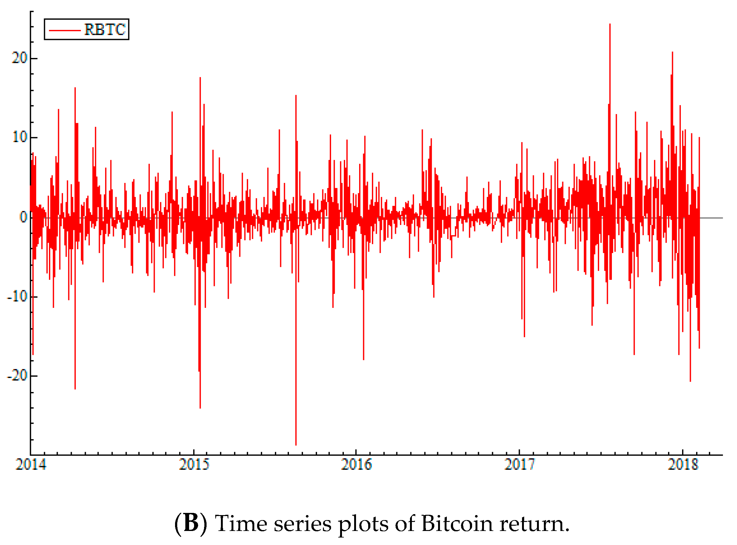
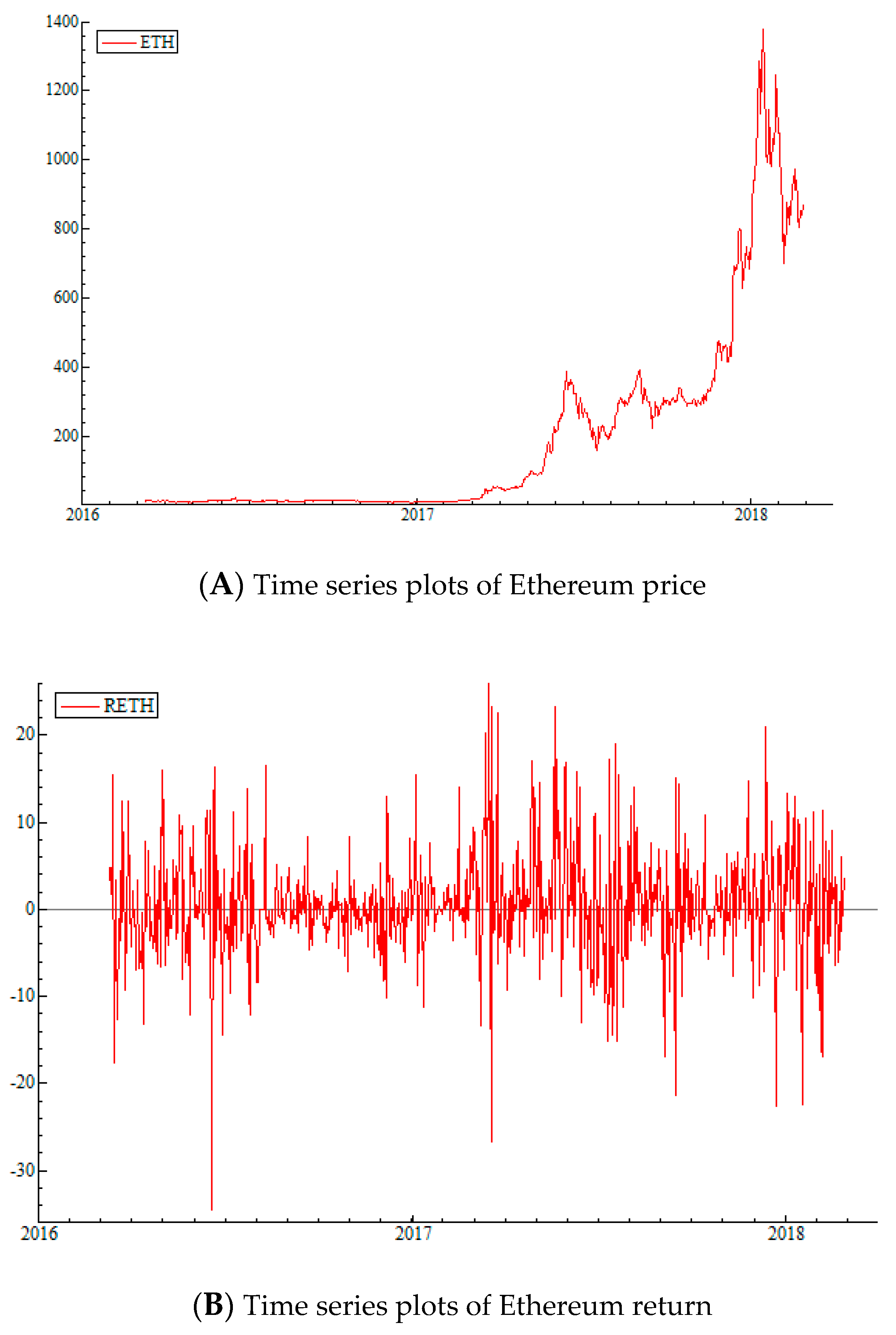
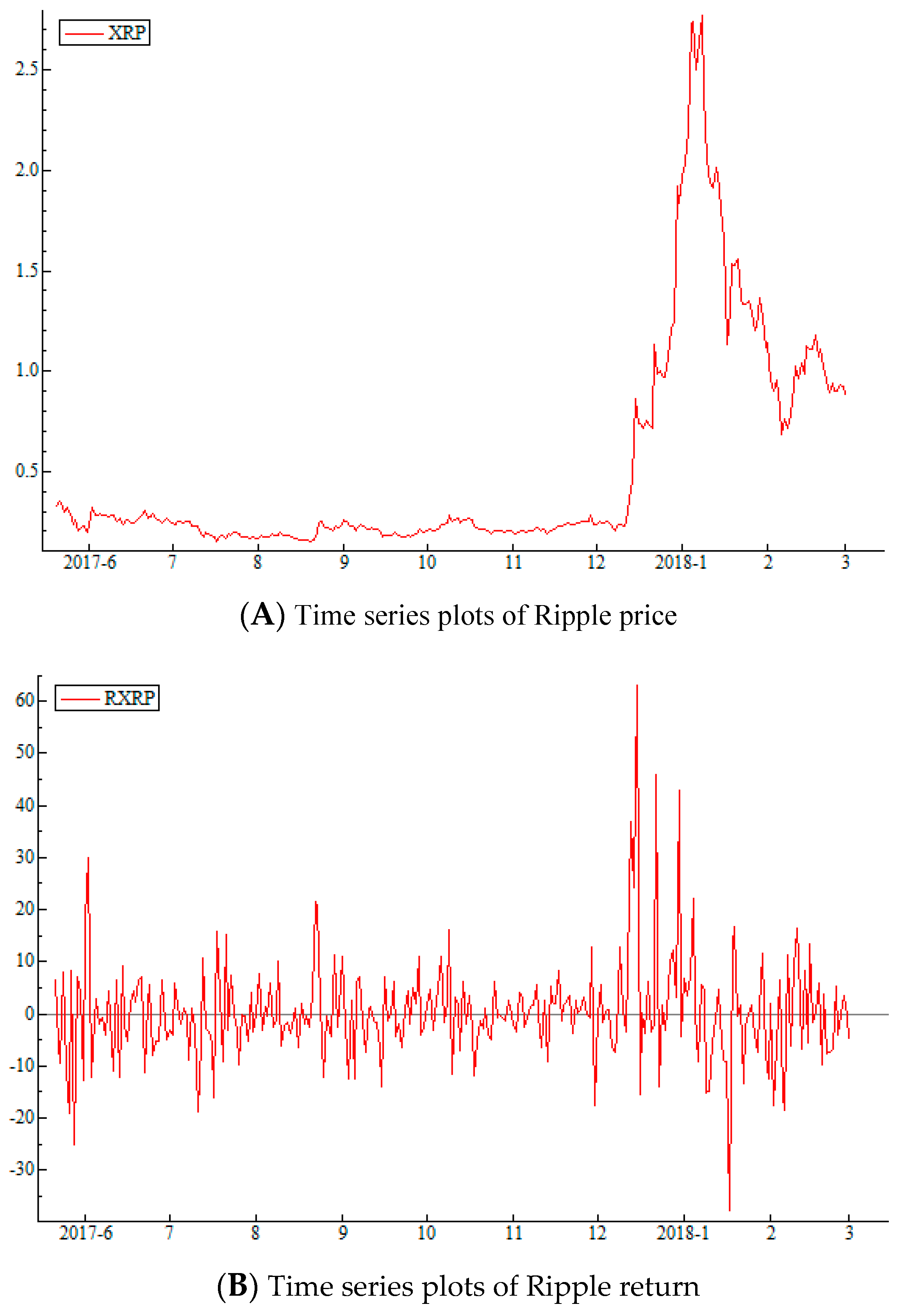
Forecasting volatility is very important for both investment decisions and risk management. However, it is possible to say that simple methods of measuring volatility, such as standard deviation, are no longer sufficient to adequately measure volatility of complex financial instruments in today’s globally integrated financial markets. At its simplest, the standard deviation gives equal weight to all past observations, which is not adequate for contemporary forecasting exercises. GARCH models, on the other hand, provide a means for measuring time-varying volatility (Engle 1982). Therefore GARCH family of volatility models have become the standard in the estimation of the volatility in financial markets and for most traditional financial instruments (Baillie 1996; Bollerslev et al. 1992; Ding and Granger 1996; Lo 1989; Pati et al. 2018; Poon and Granger 2003; Wang et al. 2018). However, since cryptocurrencies are relatively a new phenomenon, there is still not a lot of literature on the modeling of their volatility. The existing academic literature on the volatility of cryptocurrencies is limited and also focuses exclusively on the most popular cryptocurrency, Bitcoin.
For instance, Urquhart (2018) argues that the increase in transaction volume and volatility of Bitcoin are significant factors in its popularity. Caginalp and Caginalp’s (2018) findings also support Urquhart’s (2018) results about the valuation of cryptocurrencies. Iwamura et al. (2014) explores the reasons for price instability in cryptocurrencies and argues that a new monetary policy strategy without central banks could stabilize the value of Bitcoin and other cryptocurrencies. In the study, mentioning Satoshi Nakamoto’s 2008 paper, authors suggest that Bitcoin’s price inflation can be avoided by limiting the fluctuations in market value due to the previously announced limited amount of supply (Iwamura et al. 2014).
Although Bitcoin has extremely high volatility, many researchers still consider it to be a valuable diversification instrument for a portfolio (Bouri et al. 2018). Briere et al. (2015), document a low correlation between Bitcoin and both traditional assets (stocks, bonds, and hard currencies) and alternative investments (commodities, hedge funds, and real estate). Dyhrberg (2016), similarly, finds that Bitcoin can be used as a hedging instrument for UK currency and equities, since positive and negative shocks do not affect Bitcoin returns asymmetrically. Bouri et al. (2017) state that Bitcoin can serve as an effective diversifier for most of the assets and a strong hedge for the commodity market.
Recent empirical studies on cryptocurrencies focus on the long memory behavior. In their recent study, Bouri et al. (2019) investigate persistency in the price and volatility of Bitcoin. By using both parametric and semiparametric methods, they find evidence that there exists a long memory in the volatility of Bitcoin.
Chu et al. (2017) investigate the volatility of the most traded seven cryptocurrencies by using various GARCH class models. Their results show that the IGARCH and GJRGARCH models provide the best fits, in modelling the volatility in the most popular cryptocurrencies. They conclude these extreme volatility characteristics of cryptocurrencies make them interesting for the risk-seeking investors who want to enter into technology markets.
Sahoo (2017) also uses GARCH to model the volatility of Bitcoin prices, and comes to the conclusion that Bitcoin is a high volatile currency. Peng et al. (2018) try to find the best GARCH model fit that estimates volatility for three different cryptocurrencies by using daily and hourly closing price data for Bitcoin, Ethereum and Dash for the 2016–2017 period. (Peng et al. 2018). Similarly, Katsiampa (2017), also models the volatility of Bitcoin using closing prices with different GARCH models, and presents evidence of long memory in the volatility in Bitcoin prices. Lahmiri et al. (2018) show the long-term volatility of seven different cryptocurrency markets using the FIGARCH method and conclude that the volatility shocks in these markets have long memory.
Mensi et al. (2019) investigate the impacts of structural breaks on the dual long memory levels of Bitcoin and Ethereum price returns. By using four GARCH-class models (e.g., Fractional Integrated GARCH (FIGARCH), Fractional Integrated APARCH (FIAPARCH), and Hyperbolic GARCH (HYGARCH), they determine dual long memory and structural changes on cryptocurrency markets. They suggest that the FIGARCH model with structural breaks variables provides a comparatively superior forecasting accuracy performance.
In a VaR context, Likitratcharoen et al. (2018) predict the Value at Risk (VaR) of Bitcoin, Ethereum and Ripple using historical and Gaussian parametric, VaR. They use Kupiec’s proportion of failures (POF) test, independence test, and the Christoffersen (1998) and joint test in order to backtest their VaR model. Their findings show that historical VaR model is suitable for measuring cryptocurrency risk over delta normal VaR only for a high confidence level of critical values. Similarly, Osterrieder and Lorenz (2017) and Gkillas and Katsiampa (2018) apply extreme value theory to estimate VaR. Gkillas and Katsiampa (2018) analyze the tail behavior of the returns of five major cryptocurrencies in order to find while Bitcoin Cash is the riskiest cryptocurrency analyzed, Bitcoin and Litecoin are the least risky. Other studies also utilize Value-at-Risk methodologies on returns of different cyrptocurrencies to analyze their time varying-volatilities. They use methodologies based on vine copulas and robust volatility models. (Ardia et al. 2019; Stavroyiannis 2018; Troster et al. 2019; Pele and Mazurencu-Marinescu-Pele 2019; Trucíos et al. 2019).
As the literature summarized above shows, the evidence on time-varying properties of the volatility of cryptocurrency returns are fragmented. This study carries out a more comprehensive analysis by using all three of the largest market cap and most liquid cryptocurrencies (namely, Bitcoin, Ethereum, Ripple) and applying four different long-memory tests in the returns and volatilities of cryptocurrencies to investigate their stochastic properties. Moreover, after worldwide adoption of the Basel II Accord, Value at Risk (VaR) became the most widely used risk measure in quantitative finance. Value-at-Risk measures the approximate market risk of all regulated financial institutions following the Basel Accords (Alexander 2009). Therefore, investors in cryptocurrencies need to accurately predict VaR of their portfolio in order to acquire a sufficiently covered risk. Our analysis extends the findings from the literature (Chu et al. 2017) by focusing not only on the risk measurement with VaR model, but also expected shortfalls which is a coherent measure of risk.

3. Data

Most studies summarized above concentrate their GARCH models on Bitcoin only. In this paper, however, we investigate the optimal GARCH model for not only Bitcoin but also the two other major cryptocurrencies in the market: Ethereum and Ripple. The daily price data of three major crypto currencies was extracted from Bitfinex, which provides advanced services such as cryptocurrency exchange for digital currency traders and liquidity providers. Bitfinex is the world’s largest exchange by volume for trading Bitcoin against the US Dollar. In order to obtain the longest uninterrupted period possible for each cryptocurrency, we use different starting points for each. Bitcoin has the longest data stream starting from January 1, 2014, followed by Ethereum we use data starting from October 3, 2016. Finally, the data stream for Ripple starts on May 20, 2017. Data for all three cryptocurrencies end on February 28, 2018.
Daily return series are calculated as log differences of price levels as follows:
r t = 100   ×   [ l n P t l n P t 1 ]
where rt represents return at time t, lnPt is the natural logarithm of the opening price at date t and lnPt−1 is the natural logarithm of the opening price at date t − 1.
The price and return series for Bitcoin, Ethereum, and Ripple are plotted in Figure 1, Figure 2 and Figure 3, respectively. From Figure 1A, we can see that Bitcoin prices started a gradual increase at the beginning of 2017, but suddenly started rising rapidly at the end of 2017. This large and sudden increase corresponds to the introduction of the bitcoin futures trading. The return series in Figure 1B, supports the same observation. Returns of Bitcoin show high volatility all throughout the time period, however volatility spikes are bigger and more frequent after 2017. Figure 2A,B show that Ethereum prices and returns follow a very similar pattern, with increase in prices after 2017 and constantly high volatility since the beginning of trading. In the case of Ripple; however, there is no gradual price increase. According to Figure 3, the climb in Ripple prices begins with a rapid increase in December of 2017. Volatility pattern is slightly different than Bitcoin and Ethereum as well. According to Figure 3B, Ripple return volatility is relatively stable, but starts to spike after December 2017 as well.
Descriptive statistics for cryptocurrencies’ return series are shown in Table 1. Results show that all series have high excess kurtosis. Bitcoin and Ethereum have negative skewness. These statistics indicate that the distributions of the series seem to be leptokurtic. Moreover, Ljung-Box Q (20) statistics for all returns are insignificant, while it is significant for squared returns of all cryptocurrencies. Besides, regardless of the lag chosen, all ARCH (Autoregressive conditional heteroskedasticity) test statistics are highly significant. Therefore, conditional heteroscedasticity and serial correlations should be taken into account while modeling these series.

4. Methodology

In order to better detect various characteristics of cryptocurrency returns, we employ long memory tests before modeling the volatility of these series. According to the results of these long memory tests, we later estimate the appropriate GARCH class model, which accurately takes into account the asymmetry in the relevant series. Long memory process could be described as a slowly decaying autocovariance function. At this point it is necessary to remind that volatility is highly persistent in high-frequency financial time series.

4.1. Long Memory Tests

In order to test for long memory properties in these series, we employ four different statistics: The Hurst–Mandelbrot Rescaled Range (R/S) statistics; Lo (1991) Rescaled Range R/S; Geweke and Porter-Hudak (1983) (GPH); and the Robinson and Henry (1999) Gaussian Semiparametric (GSP) test statistics. Each one of these long-term memory statistics are detailed below. When testing for long-term memory for all three cryptocurrencies, we use the absolute returns and squared returns as proxies of daily volatility following Arouri et al. (2012).

4.1.1. Rescaled Range (R/S) Statistics

Rescaled range statistic R/S was introduced by Hurst (1951) and later revised by Mandelbrot and Wallis (1969) in order to detect the presence of long-term memory in time series. According to Mandelbrot (1971), R/S statistics could be used in economic and financial analysis. Essentially, rescaled range statistic R/S is the range of partial sums of deviations of a time series from its mean rescaled by its standard deviation (Zivot and Wang 2003). Consequently, Hurst exponent H symbolizes the scaling behavior of the range of cumulative departures of a time series from its mean.
Formally, the range R of a time series { x t } , t = 1 , , T is determined as:
R T = max 1 t T t = 1 T ( x t x ¯ ) min 1 t T t = 1 T ( x t x ¯ )
Here, x   ¯ is given as an estimate of the sample mean. The classical rescaled range is the best known R/S statistic:
R / S = σ ^ 1 [ max 1 t T t = 1 T ( x t x ¯ ) min 1 t T t = 1 T ( x t x ¯ ) ]   ,   σ ^ 2 = T 1 t = 1 T ( x t x ¯ ) 2
This statistic is robust to data non-normality, but in the presence of autocorrelation the coefficients may be biased. Therefore, Lo (1991) developed a modified rescaled range Q T , which adjusts for possible short term dependence by applying the Newey West heteroscedasticity and autocorrelation consistent estimator instead of the sample standard deviation S:
Q T = S T 1 [ max 1 t T t = 1 T ( x t x ¯ ) min 1 t T t = 1 T ( x t x ¯ ) ]
S T 2 = S 2 + 2 T j = 1 τ ω j ( τ ) { i = j + 1 T ( x i x ¯ ) ( x i j x ¯ ) } , ω j ( τ ) = 1 j τ + 1
Here Mandelbrot’s null hypothesis is “there is no long-term dependence” under the assumption of no autocorrelation, while Lo’s null hypothesis is only “there is no long-term dependence”.

4.1.2. Geweke and Porter-Hudak (GPH) Model

Geweke and Porter-Hudak (1983) suggested a semi-nonparametric approach to test for long-term memory in the sense of fractionally integrated processes. Furthermore, Geweke and Porter-Hudak (1983) used Fourier transformation and spectral density into the following formula.
Let r t be the return series. The GPH estimator of the long memory parameter d for r t can be then determined using the following periodogram:
log [ I ( w j ) ] = β 0 + β 1 log [ 4 sin 2 ( w j 2 ) ] + ε j
where w j = 2 π   j / T ,   j = 1 ,   2 , , n ; ε j is the residual term and w j represents the n = T Fourier frequencies. I ( w j ) stands for the sample periodogram defined as:
I ( w j ) = 1 2 π T | t = 1 T r t e w j t | 2
where r t is assumed to be a covariance stationary time series. The estimate of fractional difference parameter d, namely d ^ G P H , is β ^ 1 . GPH test for the null hypothesis is “there is no long memory (d = 0)”.

4.1.3. Gaussian Semiparametric (GSP) Method

The Gaussian Semiparametric estimation model developed by Robinson and Henry (1999) is based on the specification of the shape of the spectral density of the time series. The Robinson and Henry (1999) GSP estimator of the long memory parameter for a covariance stationary series, which is consistent and asymptotically normal under certain assumptions, is given by:
f ( w ) = G w 1 2 H   a s   w 0 +
where 1 2 < H < 1 , 0 < G < and f ( w ) is the spectral density of r t . The periodogram with respect to the observations of r t , t = 1 , , T is defined as:
I ( w j ) = 1 2 π T | t = 1 T r t e i t w j | 2
Accordingly, the Hurst exponent parameter H is obtained by minimizing the function R ( H ) .
H = arg min Δ 1 H Δ 2 R ( H )
where:
{ 0 < Δ 1 < Δ 2 < 1 R ( H ) = log { 1 m j = 1 m I ( w j ) w j 1 2 H } ( 2 H 1 ) 1 m j = 1 m log ( w j ) m ( 0 , [ n / 2 ] ) w j = 2 π j / T

4.2. Results of Long Memory Tests

Table 2, Table 3 and Table 4 provide the results of the long-range dependence tests for daily returns and daily squared returns for Bitcoin, Ethereum and Ripple, respectively. According to the four tests utilized (Hurst–Mandelbrot R/S, Lo R/S, GPH and GSP), and presented in Panels A in Table 2, Table 3 and Table 4, test statistics do not reject the null hypothesis of no long-range dependence in return series. The results indicate that daily returns for Bitcoin, Ethereum and Ripple do not exhibit the long memory effect.
Panels B in Table 2, Table 3 and Table 4, present results for the squared daily returns of these three cryptocurrencies. Long-term memory test results demonstrate the presence of the long memory effect at the 1% level. The d parameter is statistically significant and lies within the interval (0, 0.5), indicating that the squared return series exhibit long memory process.
These results are in accordance with results in previous similar studies on cryptocurrencies. Mensi et al. (2019) state that the persistence level of both returns and volatility of Bitcoin and Ethereum decrease after considering long memory and switching states. In addition, Bouri et al. (2016) show evidence of a long memory in two measures of volatility of Bitcoin. In this study, we analyze all three major cryptocurrencies that make up close to 86% of the entire cryptocurrency market cap and find that long-term memory exists in the squared terms for all three.
In short, these long-term memory test results confirm that GARCH-class models, which take into account long-term memory properties, are the most appropriate models for the volatility of Bitcoin, Ethereum and Ripple.

4.3. GARCH Models

The main assumption underlying Bollerslev’s (1986) GARCH modeling is that the market variance depends not only on historical conditional market variance but also on market shocks. Generalized Auto Regressive Conditional Heteroscedasticity (GARCH, p, q) equation is written in the following form:
R t = α 0 + i = 1 k β i X i + j = 1 h ψ j R t j + ε t
where ε t | Ω t 1 N ( 0 , h t )
h t = ω + i = 1 p β i h t i + j = 1 q α j ε t j 2
where h t = σ t 2 | Ω t 1 .
The satisfying conditions for the equations are ω > 0 , α > 0 , β 0 , ( i = 1 p α i + i = 1 q β i < 1 ) . ε t stands for disturbance term for mean equation, R t describes the return of the asset at time t, and X ’s denote explanatory variables. Equations (8) and (9) are the mean and the conditional variance equations, respectively.
In this model, in order to assure a positive conditional variance, estimated parameters should satisfy non-negativity constraints. Hence, GARCH models consider only the magnitude of the shock—not its sign.

4.3.1. The Fractional Integrated GARCH (FIGARCH) Model

Most of the time, high frequency financial data follows a pattern that yields a sum of α1 and β1 close to one, with α1 small and β1 large. Therefore, the effect of shocks on the conditional variance diminishes very slowly. In these situations, Baillie et al. (1996) suggest the class of Fractionally Integrated GARCH (FIGARCH) models. This model captures slowly decaying volatility as well as recognizing both the long memory and short memory characteristics of conditional variance (Chkili et al. 2014). Fractionally integrated processes are significantly different from both stationary and unit-root processes with their persistence and mean reverting features.
Formally, the FIGARCH (1, d, 1) can be defined with lag operator “L” as follows
h t = ω + β h t 1 + [ 1 ( 1 β L 1 ) ( 1 λ L ) ( 1 L ) d ] ε t 2
where ω > 0, β 1 and λ < 1. The fractional integration parameter d reflects the degree of long memory or the persistence of shocks to conditional variance, and satisfies the condition 0 ≤ d ≤ 1. If 0 < d < 1, the model implies an intermediate range of persistence and indicates the volatility shocks disperse only at a hyperbolic rate. If the integration parameter d = 0 then the model has a short memory and reduces to a GARCH (1,1) model. On the other hand, if d = 1, the model transforms to IGARCH (1,1) whose variance process is no longer mean-reverting (Chkili et al. 2014).

4.3.2. Hyperbolic GARCH (HYGARCH) Model

Davidson (2004) has developed a new GARCH-class model called hyperbolic GARCH (HYGARCH) model. This new model extends the conditional variance of the FIGARCH model by introducing weights into the difference operator. The HYGARCH model allows for modeling long memory property in conditional volatility with hyperbolic convergence rates. The HYGARCH (1, d,1) model can be written as follows:
h t = ω + [ 1 ( 1 β L ) 1 λ L { 1 + α ( ( 1 L ) d 1 ) } ] ε t 2
where ω > 0, α ≥ 0, β ≺ 1, λ < 1 and 0 ≤ d ≤ 1.
Davidson (2004) argues that the HYGARCH model allows for the existence of both second moments, and even more extreme amplitudes than the simple IGARCH and FIGARCH models.

4.4. The VaR and Backtesting

Value at Risk (VaR) is a risk measure that determines the losses that may happen in extreme events for a given confidence level. Main parameters of VaR are the significance level (confidence level 1-α) and the risk horizon (h), which is the period of time in terms of trading days.
VaR is an especially popular and useful tool for risk management in the sense that it measures both risk factor and the sensitivity to the same risk factor, simultaneously. VaR finds most of its universal applicability in its ability to quantify various types of risk (Alexander 2009).
VaR can identify extreme events, however it is not sub-additive, i.e., the total risk of a portfolio does not equal the sum of the risks of the individual assets. Due to this shortcoming “Expected Shortfall” has been developed as an alternative but related measure of risk (Scaillet 2000).
Expected shortfall is a risk measure, used to predict the expected value of the losses conditional on the loss being larger than the VaR (Scaillet 2004).
ESFt = E(|Lt | > |VaRt|)
where Lt is the expected value of loss if a VaRt violation occurs. Hendricks (1996) interpreted the ESF1 as the excess value of the losses over the VaR, the ESF2 as expected value of loss exceeding the VaR level, divided by the associated VaR values.
In this study, we use both long and short trading positions and estimate the relevant VaRs for the FIGARCH and HYGARCH models under the student-t and skewed student-t distributions. The daily VaR for long and short trading positions at time t can be calculated as
V a R L , t = μ t ^ + s t α σ t ^
and
V a R S , t = μ t ^ + s t 1 α σ t ^
where s t α represents the left quantile at % α for the student-t distribution and s t 1 α the right quantile at % α. μ t ^ denotes the estimated daily conditional mean whereas σ t ^ represents the estimated standard deviation of the cryptocurrency returns obtained from a FIGARCH and HYGARCH models.
The daily VaR’s for the skewed-Student-t distribution for long and short positions is given by
V a R L , t = μ t ^ + s k s t α σ t ^
and
V a R S , t = μ t ^ + s k s t 1 α σ t ^
In order to determine the accuracy of the VaR model, estimations should be backtested. This testing method enables us to compare the actual losses (or gains) in the past observations to the VaR and determine exceedances or failures. The most widely known test is Kupiec’s (1995) POF-test that examines whether the proportion of failures (POF) calculated from the data corresponds to its theoretical value.
If N = t = 1 T I t , is the number of exceptions in the sample size T, then:
I t + 1 = { 1   i f   r t + 1 < V a R t + 1 | t ( ) 0   i f r t + 1 V a R t + 1 | t ( )
where it follows a binomial distribution, N|B(T, α). If α = E(N/T) is the expected exception frequency, then the null hypothesis is whether the failure rate of the model is equal to the expected one: H0: α = α0 and where α0 is the pre-specified VaR level.
Under the null hypothesis, the Kupiec’s (1995) likelihood ratio test is given by:
L R u c = 2 l o g { α 0 N ( 1 α 0 ) T N } + 2 l o g { ( N T ) N ( 1 ( N T ) ) T N }
The Likelihood ratio statistics is asymptotically χ2 (1) chi squared distributed with one degree of freedom. If the null hypothesis, H0: α = α0, cannot be rejected, then the model will be favored for VaR prediction, which exhibits unconditional coverage measured by α = E(N/T) equals the desired coverage level α0.

5. Findings

In this part, results from the estimated GARCH-type models are presented. Student-t and skewed student-t distributions have been used since the returns have heavier tails than the normal distribution. We estimate FIGARCH, HYGARCH, FIAPARCH models with regard to long memory test results in order to account for the long memory properties of our cryptocurrency returns. However, in Table 5 we only report the best results from the various estimated GARCH models. As can be seen from the table, we fit HYGARCH, and FIGARCH both student-t and skewed student-t distributions to the return series of Bitcoin, Ethereum, and Ripple.
Especially, d-FIGARCH coefficients are statistically significant at 1% level, which implies the existence of long memory in the selected cryptocurrencies’ volatility. The values of AIC, SW, SB, and H-Quinn are given in Table 5 for the fitted models. We only include the most appropriate methods based on these information criteria and Log-likelihood statistics. However, there are small differences between these models.
The student-t distribution gives the smallest value of AIC, SW, SB, and H-Quinn with HYGARCH (1, 0.65, 1) model for Bitcoin. The best fitting model for Ethereum is the FIGARCH (1, 0.68, 1) with skewed student-t distribution. Asymmetric parameters are also positive and statistically significant for Ethereum at a 1% level, indicating that Ethereum returns are skewed to the right. In addition, the tail parameters in HYGARCH and FIGARCH models are statistically significant and positive for both Bitcoin and Ethereum. These results reveal that these two cryptocurrencies are fat-tailed. The student-t distribution gives the smallest values of information criteria for Ripple returns. Thus, we may suggest that FIGARCH (1, 0.625, 1) is the best fitting model for Ripple.

In Sample VaR Estimations

In this section, the GARCH models were tested for VaR levels ranging from 5% to 1%. Table 6 displays the in-sample VaR estimations which are calculated from FIGARCH and HYGARCH models for daily returns of Bitcoin, Ethereum and ripple, respectively. The Kupiec tests are conducted for each of these models in order to investigate whether the empirical failure rate is equal to the pre-specified VaR level.
The Kupiec test statistics are not significant in most cases, indicating that the FIGARCH and HYGARCH models perform well in estimating the volatility of these cryptocurrency returns. Kupiec test statistics is only significant at 5% level for Ethereum and 1% level for Ripple in short positions. Moreover, the Kupiec test statistics are not statistically significant for any of the three cryptocurrencies for long trading positions. More precisely, the results show that the FIGARCH and HYGARCH models with skewed student t distributions outperform the other methods.
The next risk measure considered for the three cryptocurrencies is Expected Shortfalls (ESF). The expected shortfall results for long and short positions are identified as ESF1 and ESF2, respectively, and are presented in Table 7.
According to our findings, expected shortfalls are the highest for Ripple and lowest for Bitcoin for all risk levels. In conclusion, investors should be aware that Ethereum and Ripple are subject to a much higher risk than Bitcoin and may require higher capital to cover for potential losses.

6. Conclusions

Volatility of various assets in financial markets has been broadly analyzed in the finance literature. However, there exists little empirical research on modelling volatility and investigating long memory property of cryptocurrencies. Studies on cryptocurrencies has recently prompted the interest of researchers as their use has increased adequately.
The main purpose of this study is to model the volatility of the mostly mined cryptocurrencies: Bitcoin, Ethereum, and Ripple. By modelling volatility, we take into account long memory properties of these cryptocurrencies. This gives us the opportunity to examine market efficiency. Similar to previous researches, Cheah et al. (2018), Bouri et al. (2019) and Mensi et al. (2019), our findings also indicate that cryptocurrency market has a long memory and that such a memory implies inefficiency in the market where the estimated memory in volatility can help investors capture speculative profits.
From the price data, it can be observed that cryptocurrencies are highly volatile especially over the period spanning between July 2017 and February 2018. In addition, our findings indicate that HYGARCH model appears to be the best fitted model for Bitcoin as reported by the AIC, SW, SB and H-Quinn criteria, and Log likelihood. Considering long memory also improves the performance of modelling cryptocurrencies with GARCH models. On the other hand, the FIGARCH model with skewed student distribution produces better estimations for Ethereum. Further, FIGARCH model with student distribution appears to give a good fit for Ripple return. All of the series for the selected cryptocurrencies exhibit fat-tail problem which may be a sign for the probability that an investment return in the selected cryptocurrencies may move beyond three standard deviations.
Other studies dealing with cryptocurrencies also attain almost identical results: Bouri et al. (2019) found long memory in the volatility of Bitcoin. Mensi et al. (2019) argued that FIGARCH model with structural breaks variables outperforms the other models in the forecasting accuracy performance. Lahmiri et al. (2018) suggested that the FIGARCH model is the best suited for estimating the volatility and volatility shocks in these markets have long memory. Moreover, like previous study of Stavroyiannis (2018), VaR and expected shortfall analysis show that the capital requirements of the cryptocurrencies are high. In conclusion, models which take into account volatility clustering, asymmetry and long memory in the cryptocurrency volatilities predict more accurately the VaR and ESF for both the short and the long trading positions.
The findings of this research will help investors and especially the institutional investors in developing investment strategies by providing cryptocurrencies as a potential investment instrument in order to achieve a better portfolio diversification. Furthermore, as the three of the cryptocurrencies selected for this research cover 86% of market cap and more than 60% of trading volume in the recent years, the findings of this study could also be a good benchmark point for the institutional investors dealing with the other cryptocurrencies.
Cryptocurrencies might become a mainstream financial instrument in the future of the global financial markets besides common stocks, commodities and precious metals or Fx instruments. Thus, this research will also provide investors with a better understanding of the cryptocurrencies markets and will encourage further studies.

Author Contributions

Conceptualization, P.K.S., M.O., Ö.Ç. and Z.A.A.; methodology, P.K.S.; formal analysis, P.K.S.; writing—original draft preparation, P.K.S. and M.O.; writing—review and editing, P.K.S., M.O. and Z.A.A.; supervision Ö.Ç.; funding acquisition, Z.A.A. All authors have read and agreed to the published version of the manuscript.

Funding

APC was funded by Claremont Graduate University.

Conflicts of Interest

The authors declare no conflict of interest.

References

  1. Alexander, Carol. 2009. Market Risk Analysis, Value at Risk Models. Hoboken: John Wiley & Sons. [Google Scholar]
  2. Allen, Franklin, and Elena Carletti. 2010. An overview of the crisis: Causes, consequences, and solutions. International Review of Finance 10: 1–26. [Google Scholar] [CrossRef]
  3. Ardia, David, Keven Bluteau, and Maxime Rüede. 2019. Regime changes in Bitcoin GARCH volatility dynamics. Finance Research Letters 29: 266–71. [Google Scholar] [CrossRef]
  4. Arouri, Mohamed, Shawkat Hammoudeh, Amine Lahiani, and Duc Khuong Nguyen. 2012. Long memory and structural breaks in modeling the return and volatility dynamics of precious metals. The Quarterly Review of Economics and Finance 52: 207–18. [Google Scholar] [CrossRef] [Green Version]
  5. Baillie, Richard, Tim Bollerslev, and Hans Ole Mikkelsen. 1996. Fractionally integrated generalized autoregressive conditional heteroskedasticity. Journal of Econometrics 74: 3–30. [Google Scholar] [CrossRef]
  6. Baillie, Richard. 1996. Long memory processes and fractional integration in econometrics. Journal of Econometrics 73: 5–59. [Google Scholar] [CrossRef]
  7. Barber, Simon, Xavier Boyen, Elaine Shi, and Ersin Uzun. 2012. Bitter to better—how to make bitcoin a better currency. In International Conference on Financial Cryptography and Data Security. Berlin/Heidelberg: Springer. [Google Scholar]
  8. BitInfoCharts. 2018. Cryptocurrency Chart. Available online: https://bitinfocharts.com/cryptocurrency-charts.html (accessed on 1 March 2018).
  9. Blanchard, Olivier. 2016. Currency wars, coordination, and capital controls. National Bureau of Economic Research 13: 283–308. [Google Scholar]
  10. Bollerslev, Tim. 1986. Generalized autoregressive conditional heteroskedasticity. Journal of Econometrics 31: 307–27. [Google Scholar] [CrossRef] [Green Version]
  11. Bollerslev, Tim, Ray Chou, and Kenneth F. Kroner. 1992. ARCH modeling in finance: A review of the theory and empirical evidence. Journal of Econometrics 52: 5–59. [Google Scholar] [CrossRef]
  12. Bordo, Michael D., and Pierre L. Siklos. 2017. Central Bank Credibility before and after the Crisis. Open Economies Review 28: 19–45. [Google Scholar] [CrossRef] [Green Version]
  13. Bouri, Elie, Georges Azzi, and Anne Haubo Dyhrberg. 2016. Bouri, Elie and Azzi, Georges and Dyhrberg, Anne Haubo, On the Return-Volatility Relationship in the Bitcoin Market around the Price Crash of 2013. Available at SSRN 2869855. [Google Scholar] [CrossRef] [Green Version]
  14. Bouri, Elie, Luis A. Gil-Alana, R. Gupta, and David Roubaud. 2019. Modelling long memory volatility in the Bitcoin market: Evidence of persistence and structural breaks. International Journal of Finance & Economics 24: 412–26. [Google Scholar]
  15. Bouri, Elie, Peter Molnár, Geoges Azzi, David Roubaud, and Lars Ivar Hagfors. 2017. On the hedge and safe haven properties of Bitcoin: Is it really more than a diversifier? Finance Research Letters 20: 192–98. [Google Scholar] [CrossRef]
  16. Bouri, Elie, Rangan Gupta, Chi Keung Lau, David Roubaud, and Shixuan Wang. 2018. Bitcoin and global financial stress: A copula-based approach to dependence and causality in the quantiles. The Quarterly Review of Economics and Finance 69: 297–307. [Google Scholar] [CrossRef] [Green Version]
  17. Briere, Marie, Kim Oosterlinck, and Ariane Szafarz. 2015. Virtual currency, tangible return: Portfolio diversification with bitcoin. Journal of Asset Management 16: 365–73. [Google Scholar] [CrossRef]
  18. Caballero, Ricardo, Emanuel Farhi, and Pierre-Olivier Gourinchas. 2015. Global Imbalances and Policy Wars at the Zero Lower Bound. NBER Working Paper No. 21670. London, UK: CEPR. [Google Scholar]
  19. Caginalp, Carey, and Gunduz Caginalp. 2018. Opinion: Valuation, liquidity price, and stability of cryptocurrencies. Proceedings of the National Academy of Sciences 115: 1131–34. [Google Scholar] [CrossRef] [Green Version]
  20. Çağlar, Ünal. 2007. Elektronik Para: Enformasyon Teknolojisindeki Gelişmeler ve Yeni Ödeme Sistemleri. Kırgızistan Türkiye Manas Üniversitesi Sosyal Bilimler Dergisi 17: 9. [Google Scholar]
  21. Carmassi, Jacopo, Daniel Gros, and Stefano Micossi. 2009. The global financial crisis: Causes and cures. JCMS: Journal of Common Market Studies 47: 977–96. [Google Scholar] [CrossRef]
  22. Catania, Leopoldo, Stefano Grassi, and Francesco Ravazzolo. 2018. Predicting the volatility of cryptocurrency time-series. In Mathematical and Statistical Methods for Actuarial Sciences and Finance. Berlin/Heidelberg: Springer, pp. 203–7. [Google Scholar]
  23. Cheah, Eng-Tuck, Tapas Mishra, Mamata Parhi, and Zhuang Zhang. 2018. Long memory interdependency and inefficiency in Bitcoin markets. Economics Letters 167: 18–25. [Google Scholar] [CrossRef]
  24. Chkili, Walid, Shawkat Hammoudeh, and Duc Khuong Nguyen. 2014. Volatility forecasting and risk management for commodity markets in the presence of asymmetry and long memory. Energy Economics 41: 1–18. [Google Scholar] [CrossRef]
  25. Christoofersen, Peter F. 1998. Evaluating interval forecasts. International Economic Review 39: 841–62. [Google Scholar] [CrossRef]
  26. Chu, Jeffrey, Stephen Chan, Saralees Nadarajah, and Joerg Osterrieder. 2017. GARCH modelling of cryptocurrencies. Journal of Risk and Financial Management 10: 17. [Google Scholar] [CrossRef]
  27. Cline, William R., and John Williamson. 2010. Currency wars? Policy Briefs in International Economics, 10–26. [Google Scholar]
  28. Cukierman, Alex. 2013. Monetary policy and institutions before, during, and after the global financial crisis. Journal of Financial Stability 9: 373–84. [Google Scholar] [CrossRef]
  29. Davidson, James. 2004. Moment and memory properties of linear conditional heteroscedasticity models, and a new model. Journal of Business & Economic Statistics 22: 16–29. [Google Scholar]
  30. Ding, Zhuanxin, and Clive W. J. Granger. 1996. Modeling volatility persistence of speculative returns: A new approach. Journal of Econometrics 73: 185–215. [Google Scholar] [CrossRef]
  31. Dominguez, Kathryn M. E., Yuko Hashimoto, and Takatoshi Ito. 2012. International reserves and the global financial crisis. Journal of International Economics 88: 388–406. [Google Scholar] [CrossRef]
  32. Dyhrberg, Anna Haubo. 2016. Bitcoin, gold and the dollar–A GARCH volatility analysis. Finance Research Letters 16: 85–92. [Google Scholar] [CrossRef] [Green Version]
  33. Engle, Robert F. 1982. Autoregressive conditional heteroscedasticity with estimates of the variance of United Kingdom inflation. Econometrica: Journal of the Econometric Society, 987–1007. [Google Scholar] [CrossRef]
  34. Geweke, John, and Susan Porter-Hudak. 1983. The estimation and application of long memory time series models. Journal of Time Series Analysis 4: 221–38. [Google Scholar] [CrossRef]
  35. Gil-Alana, Luis Alberiko, Olanrewaju L. Shittu, and OlaOluwa Simon Yaya. 2014. On the persistence and volatility in European, American and Asian stocks bull and bear markets. Journal of International Money and Finance 40: 149–62. [Google Scholar] [CrossRef] [Green Version]
  36. Gkillas, Konstantinos, and Paraskevi Katsiampa. 2018. An application of extreme value theory to cryptocurrencies. Economics Letters 164: 109–11. [Google Scholar] [CrossRef] [Green Version]
  37. Hendricks, Darryll. 1996. Evaluation of value-at-risk models using historical data. Economic Policy Review 2: 1. [Google Scholar] [CrossRef] [Green Version]
  38. Hileman, Garrick, and Michel Rauchs. 2017. Global cryptocurrency benchmarking study. In Cambridge Centre for Alternative Finance. Cambridge: Cambridge Judge Business School, University of Cambridge. [Google Scholar]
  39. Hurst, Harold E. 1951. Long-term storage capacity of reservoirs. Transactions of the American Society of Civil Engineers 116: 770–99. [Google Scholar]
  40. Iwamura, Mitsuru, Yukinobu Kitamura, Tsutomu Matsumoto, and Kenji Saito. 2014. Can we stabilize the price of a Cryptocurrency: Understanding the design of Bitcoin and its potential to compete with Central Bank money. Hitotsubashi Journal of Economics, 41–46. [Google Scholar] [CrossRef] [Green Version]
  41. Jackson, Olly. 2018. Confusion reigns: Are cryptocurrencies commodities or securities? International Financial Law Review 1: 1. [Google Scholar]
  42. Katsiampa, Paraskevi. 2017. Volatility estimation for Bitcoin: A comparison of GARCH models. Economics Letters 158: 3–6. [Google Scholar] [CrossRef] [Green Version]
  43. Kupiec, Paul H. 1995. Techniques for verifying the accuracy of risk measurement models. The Journal of Derivatives 3: 73–84. [Google Scholar] [CrossRef]
  44. Lahmiri, Salim, Stelio Bekiros, and Antonio Salvi. 2018. Long-range memory, distributional variation and randomness of bitcoin volatility. Chaos, Solitons & Fractals 107: 43–48. [Google Scholar]
  45. Likitratcharoen, Danai, Teerasak Na Ranong, Ratikorn Chuengsuksomboon, Norrasate Sritanee, and Ariyapong Pansriwong. 2018. Value at risk performance in cryptocurrencies. The Journal of Risk Management and Insurance 22: 11–28. [Google Scholar]
  46. Liu, Yukun, and Aleh Tsyvinski. 2018. Risks and returns of cryptocurrency. National Bureau of Economic Research. [Google Scholar] [CrossRef]
  47. Lo, Andrew W. 1989. Long-Term Memory in Stock Market Prices. NBER Working Paper No. 2984. Cambridge, MA, USA: National Bureau of Economic Research. [Google Scholar]
  48. Lo, Andrew W. 1991. Long-Term Memory in Stock Market Prices. Econometrica 59: 1279–313. [Google Scholar] [CrossRef]
  49. Malkiel, Burton G., and Eugene F. Fama. 1970. Efficient capital markets: A review of theory and empirical work. The Journal of Finance 25: 383–417. [Google Scholar] [CrossRef]
  50. Mandelbrot, Benoit, and James R. Wallis. 1969. Robustness of the rescaled range R/S in the measurement of noncyclic long run statistical dependence. Water Resources Research 5: 967–88. [Google Scholar] [CrossRef]
  51. Mandelbrot, Benoit. 1971. When can price be arbitraged efficiently? A limit to the validity of the random walk and martingale models. The Review of Economics and Statistics 53: 225–36. [Google Scholar] [CrossRef]
  52. Mensi, Walid, Khamis Hamed Al-Yahyaee, and Sang Hoon Kang. 2019. Structural breaks and double long memory of cryptocurrency prices: A comparative analysis from Bitcoin and Ethereum. Finance Research Letters 29: 222–30. [Google Scholar] [CrossRef]
  53. Osterrieder, Joerg, and Julian Lorenz. 2017. A statistical risk assessment of Bitcoin and its extreme tail behavior. Annals of Financial Economics 12: 1750003. [Google Scholar] [CrossRef]
  54. Panagiotidis, Theodore, Thanasis Stengos, and Orestis Vravosinos. 2018. On the determinants of bitcoin returns: A LASSO approach. Finance Research Letters 27: 235–40. [Google Scholar] [CrossRef]
  55. Panagiotidis, Theodore, Thanasis Stengos, and Orestis Vravosinos. 2019. The effects of markets, uncertainty and search intensity on bitcoin returns. International Review of Financial Analysis 63: 220–42. [Google Scholar] [CrossRef]
  56. Panagiotidis, Theodore, Thanasis Stengos, and Orestis Vravosinos. 2020. A Principal Component-Guided Sparse Regression Approach for the Determination of Bitcoin Returns. Journal of Risk and Financial Management 13: 33. [Google Scholar] [CrossRef] [Green Version]
  57. Pati, Pratap Chandra, Parama Barai, and Prabina Rajib. 2018. Forecasting stock market volatility and information content of implied volatility index. Applied Economics 50: 2552–68. [Google Scholar] [CrossRef]
  58. Pele, Daniel Traian, and Miruna Mazurencu-Marinescu-Pele. 2019. Using high-frequency entropy to forecast Bitcoin’s daily Value at Risk. Entropy 21: 102. [Google Scholar] [CrossRef] [Green Version]
  59. Peng, Yaohao, Pedro Henrique Melo Albuquerque, Jader Martins Camboim de Sá, Ana Julia Akaishi Padula, and Mariana Rosa Montenegro. 2018. The best of two worlds: Forecasting high frequency volatility for cryptocurrencies and traditional currencies with Support Vector Regression. Expert Systems with Applications 97: 177–92. [Google Scholar] [CrossRef]
  60. Poon, Ser-Huang, and Clive W. J. Granger. 2003. Forecasting volatility in financial markets: A review. Journal of Economic Literature 41: 478–539. [Google Scholar] [CrossRef]
  61. Robinson, P. M., and Marc Henry. 1999. Long and short memory conditional heteroskedasticity in estimating the memory parameter of levels. Econometric Theory 15: 299–336. [Google Scholar] [CrossRef] [Green Version]
  62. Sahoo, Pradipta Kumar. 2017. Bitcoin as digital money: Its growth and future sustainability. Theoretical & Applied Economics 24: 53–64. [Google Scholar]
  63. Scaillet, Olivier. 2000. Nonparametric Estimation and Sensitivity Analysis of Expected Shortfall. Louvain-la-Neuve: Université Catholique de Louvain. [Google Scholar]
  64. Scaillet, Olivier. 2004. Nonparametric estimation and sensitivity analysis of expected shortfall. Mathematical Finance: An International Journal of Mathematics. Statistics and Financial Economics 14: 115–29. [Google Scholar]
  65. Stavroyiannis, Stavro. 2018. Value-at-risk and related measures for the Bitcoin. The Journal of Risk Finance. [Google Scholar] [CrossRef]
  66. Troster, Victor, Aviral Kumar Tiwari, Muhammad Shahbaz, and Demian Nicolas Macedo. 2019. Bitcoin returns and risk: A general GARCH and GAS analysis. Finance Research Letters 30: 187–93. [Google Scholar] [CrossRef]
  67. Trucíos, Carlos, Aviral K. Tiwari, and Faisal Alqahtani. 2019. Value-at-risk and expected shortfall in cryptocurrencies’ portfolio: A vine copula–based approach. Applied Economics, 1–14. [Google Scholar] [CrossRef]
  68. Urquhart, Andrew. 2018. What causes the attention of Bitcoin? Economics Letters 166: 40–44. [Google Scholar] [CrossRef] [Green Version]
  69. Wagner, Helmut. 2010. The causes of the recent financial crisis and the role of central banks in avoiding the next one. International Economics and Economic Policy 7: 63–82. [Google Scholar] [CrossRef]
  70. Wang, Yudong, Zhiyuan Pan, and Chongfeng Wu. 2018. Volatility spillover from the US to international stock markets: A heterogeneous volatility spillover GARCH model. Journal of Forecasting 37: 385–400. [Google Scholar] [CrossRef]
  71. Zivot, Eric, and Jiahui Wang. 2003. Rolling analysis of time series. In Modeling Financial Time Series with S-Plus®. New York: Springer, pp. 299–346. [Google Scholar]
Figure 1. Time Series Plots of Bitcoin price and return. (A) Presents the plot historical plot of daily closing prices for Bitcoin between January 1, 2014 and February 28, 2018. (B) Presents the daily returns for Bitcoin for the same time period. The data is obtained from Bitfinex.
Jrfm 13 00107 g001aJrfm 13 00107 g001b
Figure 2. Time Series Plots of Ethereum Price and Return. (A) Presents the plot historical plot of daily closing prices for Ethereum between October 3, 2016 and February 28, 2018; (B) presents the daily returns for Ethereum for the same time period. The data is obtained from Bitfinex.
Jrfm 13 00107 g002
Figure 3. Time Series Plots of Ripple Price and Return. (A) Presents the plot historical plot of daily closing prices for Ripple between May 20, 2017 and February 28, 2018; (B) presents the daily returns for Ripple for the same time period. The data is obtained from Bitfinex.
Jrfm 13 00107 g003
Table 1. Descriptive Statistics.
StatisticBTCETHXRP
Mean0.1580.6050.351
Maximum24.34825.85963.137
Minimum−28.703−34.48−37.713
Std. Dev.4.096.6139.859
Skewness−0.442−0.0761.54
Kurtosis9.8736.36311.715
Jarque-Bera2951.355339.7071014.636
ARCH 1-252.23 ***49.4 ***6.16 ***
ARCH 1-525.45 ***22.42 ***2.88 ***
ARCH 1-1014.02 ***11.83 ***4.33 ***
Q(20)27.7522.6226.94
Qsq(20)212.32 ***159.79 ***69.52 ***
Observations1475719285
Table 1 provides the descriptive statistics for the returns of Bitcoin, Ethereum and Ripple daily returns. BTC represents Bitcoin, ETH represents Ethereum and XRP represents Ripple. BTC data series starts on January 1, 2014, ETH data series starts on October 3, 2016 and the Ripple data series starts on May 20, 2017. All series end on February 28, 2018. In addition to traditional descriptive statistics, the table also provides the ARCH 1-2, ARCH 1-5 and ARCH 1-10 estimations and Ljung-Box Q20 statistics for the returns and squared returns for each of the cryptocurrencies. *, **, *** represent statistical significance at 10%, 5% and 1% levels, respectively.
Table 2. Long Memory Tests for Bitcoin (BTC) Return and Squared Return.
Panel 2A: Bitcoin (BTC) Daily Returns
StatisticHurst–Mandelbrot R/SLo R/SGPHGSP
d parameter--–0.027 (0.025)–0.01 (0.018)
Test Statistics2.0942.117
Critical values ProbabilityProbability
90%[0.861, 1.747] [0.2722][0.5635]
95%[0.809, 1.862]
99%[0.721, 2.098]
Panel 2B: Bitcoin (BTC) Squared Daily Returns
StatisticHurst–Mandelbrot R/SLo R/SGPHGSP
d parameter--0.175 (0.025)0.175 (0.018)
Test Statistics3.2522.900
Critical values ProbabilityProbability
90%[0.861, 1.747] [0.0000][0.0000]
95%[0.809, 1.862]
99%[0.721, 2.098]
This table provides the results of the four different long-term memory tests run on daily returns of Bitcoin and squared daily returns of Bitcoin between January 1, 2014 and February 28, 2018. The 4 different long memory test results presented are: Hurst–Mandelbrot Rescaled Range (R/S) statistics, Lo (1991) Rescaled Range R/S statistics, Geweke and Porter-Hudak (1983) (GPH) statistics, and the Robinson and Henry (1999) Gaussian Semiparametric (GSP) test statistics. Panel 2 A presents the results for Bitcoin daily returns and Panel 2B represents the results for squared daily Bitcoin returns.
Table 3. Long Memory Tests for Ethereum Return and Squared Return.
Panel 3A: Ethereum (ETH) Daily Returns
StatisticHurst–Mandelbrot R/SLo R/SGPHGSP
d parameter--0.034 (0.038)0.022 (0.026)
Test Statistics1.6761.665
Critical values ProbabilityProbability
90%[0.861, 1.747] [0.3796][0.3963]
95%[0.809, 1.862]
99%[0.721, 2.098]
Panel 3B: Ethereum (ETH) Squared Daily Returns
StatisticHurst–Mandelbrot R/SLo R/SGPHGSP
d parameter--0.264 (0.038)0.255 (0.026)
Test Statistics2.4822.139
Critical values ProbabilityProbability
90%[0.861, 1.747] [0.0000][0.0000]
95%[0.809, 1.862]
99%[0.721, 2.098]
This table provides the results of the four different long-term memory tests run on daily returns of Ethereum and squared daily returns of Ethereum between October 3, 2016 and February 28, 2018. The 4 different long memory test results presented are: Hurst–Mandelbrot Rescaled Range (R/S) statistics, Lo (1991) rescaled Range R/S statistics, Geweke and Porter-Hudak (1983) (GPH) statistics, and the Robinson and Henry (1999) Gaussian Semiparametric (GSP) test statistics. Panel 3A presents the results for Ethereum daily returns and Panel 3B represents the results for squared daily Ethereum returns.
Table 4. Long Memory Tests for Ripple Return and Squared Return.
Panel 4A: Ripple (XRP) Daily Returns
StatisticHurst–Mandelbrot R/SLo R/SGPHGSP
d parameter--0.076 (0.063)0.038 (0.041)
Test Statistics1.4961.492
Critical values ProbabilityProbability
90%[0.861, 1.747] [0.2298][0.3613]
95%[0.809, 1.862]
99%[0.721, 2.098]
Panel 4B: Ripple (XRP) Squared Daily Returns
StatisticHurst–Mandelbrot R/SLo R/SGPHGSP
d parameter--0.18 (0.063)0.122 (0.041)
Test Statistics2.0111.887
Critical values ProbabilityProbability
90%[0.861, 1.747] [0.0047][0.0035]
95%[0.809, 1.862]
99%[0.721, 2.098]
This table provides the results of the four different long-term memory tests run on daily returns of Ripple and squared daily returns of Ripple between October 3, 2016 and February 28, 2018. The four different long memory test results presented are: Hurst–Mandelbrot Rescaled Range (R/S) statistics, Lo (1991) Rescaled Range R/S statistics, Geweke and Porter-Hudak (1983) (GPH) statistics, and the Robinson and Henry (1999) Gaussian Semiparametric (GSP) test statistics. Panel 4A presents the results for Ripple daily returns and Panel 4B represents the results for squared daily Ripple returns.
Table 5. Estimation Results of Bitcoin, Ethereum, and Ripple returns.
Estimation MethodBTCETHXRP
HYGARCH
Student
HYGARCH
sk.-t
FIGARCH
sk.-t
HYGARCH
sk.-t
FIGARCH
Student
FIGARCH
sk.-t
Cst(M)0.145 ***0.114 **0.368 **0.351 **−0.1920.092
Cst(V)0.1280.146272.831.1270.7220.377
d-Figarch0.65 ***0.659 ***0.68 ***0.643 **0.625 **0.60 **
ARCH(Alpha1)0.207 **0.201 **0.281 **0.3260.594 ***0.586 ***
GARCH(Beta1)0.678 ***0.68 ***0.636 ***0.633 ***0.896 ***0.903 ***
Student(DF)2.737 *** 3.584 ***
Asymmetry -0.0230.103 ***0.098 *** 0.104
Tail 2.739 ***4.115 ***3.73 *** 3.648 ***
Log Alpha (HY)0.241 **0.238 ** 0.106
No. Observations14751475719719285285
No. Parameters787867
Log Likelihood−3758.126−3757.843−2256.649−2256.91−994.076−993.21
AIC5.1055.1066.2966.307.0187.019
SW5.1305.1346.3416.3517.0947.108
SB5.1055.1066.2966.297.0177.017
H-Quinn5.1145.1166.3136.3197.0487.054
JB3429835411177.96168.64210.67281.64
Nyblom stability test3.9644.1521.9891.6791.0701.171
Pearson (50)54.322 *53.847 *81.486 ***67.30 ***49.91248.50
This table presents the results of various estimated GARCH type models. HYGARCH, and FIGARCH models with both student t and skewed student t distributions are fitted to all three return series. Models with the best outcomes are presented. BTC, ETH and XRP represent the daily return series for Bitcoin, Ethereum and Ripple respectively. BTC data series starts on January 1, 2014, ETH data series starts on October 3, 2016 and the Ripple data series starts on May 20, 2017. All series end on February 28, 2018. Sk.-t is the skewed Student-t distribution. *, ** and *** indicate statistical significance at the 10%, 5% and 1% levels respectively.
Table 6. In-sample Value-at-Risk (VaR) Backtesting for Cryptocurrency Returns.
Panel A: VaR Backtesting Results for Bitcoin (BTC) Returns.
BTC HYGARCH sk.-tBTC HYGARCH
Short positionsShort positions
QuantileSuccess rateKupiec LRTP-valueSuccess rateKupiec LRTP-value
0.950.9470.2530.6140.9510.0440.833
0.9750.9740.0340.8510.9740.03480.851
0.990.9890.1040.7460.9890.10410.746
Long positionsLong positions
QuantileFailure rateKupiec LRTP-valueFailure rateKupiec LRTP-value
0.050.0540.7280.3930.0571.7250.188
0.0250.0230.0990.7520.0250.00040.983
0.010.0100.0040.9470.0100.0040.947
Panel B: VaR Backtesting Results for Ethereum (ETH) Returns.
ETH FIGARCH sk.-tETH HYGARCH sk.-t
Short positionsShort positions
QuantileSuccess rateKupiec LRTP-valueSuccess rateKupiec LRTP-value
0.950.9333.864 **0.0490.9362.727 *0.098
0.9750.9730.0580.8080.9790.5340.464
0.990.9880.0880.7650.9910.2100.646
Long positionsLong positions
QuantileFailure rateKupiec LRTP-valueFailure rateKupiec LRTP-value
0.050.0581.0190.3120.0510.0310.858
0.0250.0300.8630.3520.0260.0580.808
0.010.0110.0880.7650.0090.0050.942
Panel C: VaR Backtesting Results for Ripple (XRP) Returns.
XRP FIGARCHXRP FIGARCH sk.-t
Short positionsShort positions
QuantileSuccess rateKupiec LRTP-valueSuccess rateKupiec LRTP-value
0.950.9331.5150.2180.9400.5270.467
0.9750.9680.4670.4940.9680.4670.494
0.990.9754.341 **0.0370.9821.3370.247
Long positionsLong positions
QuantileFailure rateKupiec LRTP-valueFailure rateKupiec LRTP-value
0.050.0450.1180.7300.0520.0400.839
0.0250.0170.7240.3940.0280.1060.744
0.010.0070.2850.5920.0100.0070.929
Panels A, B and C represent the VaR backtesting results for Bitcoin, Ethereum and Ripple, respectively using the models presented in Table 5. BTC data series starts on January 1, 2014, ETH data series starts on October 3, 2016 and the Ripple data series starts on May 20, 2017. All series end on February 28, 2018. The table reports the Kupiec test statistics. Both short and long position VaRs are tested. Sk.-t is the skewed Student-t distribution. *, ** and *** indicate that statistics are significance at the 10%, 5% and 1% level of significant respectively. The best model is the one with the least rejections.
Table 7. In-sample Value-at-Risk (VaR) Expected Shortfalls.
Panel A: Expected Shortfalls for Bitcoin (BTC).
BTCHYGARCHHYGARCHsk.-t
α quantileESF1ESF2ESF1ESF2
Short positions
0.957.72251.55867.53191.5416
0.979.01071.43349.01071.4624
0.999.68571.23159.68571.26
Long positions
0.05–8.721.6721–8.881.6717
0.025–11.081.6698–11.381.6709
0.01–13.461.5745–13.461.537
Panel B: Expected Shortfalls for Ethereum (ETH).
ETHFIGARCHHYGARCHsk.-t
α quantileESF1ESF2ESF1ESF2
Short positions
0.9513.81.366313.931.33
0.97151.325515.151.3606
0.9915.921.221316.591.2115
Long positions
0.05−12.621.4874−13.251.4821
0.025−14.191.3998−15.031.3772
0.01−19.481.3946−20.111.3148
Panel C: Expected Shortfalls for Ripple (XRP).
XRPFIGARCHFIGARCHsk.-t
α quantileESF1ESF2ESF1ESF2
Short positions
0.9522.441.63523.521.6362
0.9731.351.677831.351.607
0.9934.191.331242.071.4082
Long positions
0.05−17.241.3569−16.841.4136
0.025−23.051.2638−20.021.2529
0.01−28.261.0676−27.221.1236
Panels A, B and C represent the VaR backtesting Expected Shortfalls for Bitcoin, Ethereum and Ripple, respectively using the models presented in Table 5. BTC data series starts on January 1, 2014, ETH data series starts on October 3, 2016 and the Ripple data series starts on May 20, 2017. All series end on February 28, 2018. Expected Shortfalls for both long and short positions are presented. ESF 1 represents the excess value of losses above the VaR level and ESF 2 represents the expected value of losses exceeding the VaR level divided by the associated VaR values.

