Forest of Stochastic Trees: A Method for Valuing Multiple Exercise Options

Abstract

We present the Forest of Stochastic Trees (FOST) method for pricing multiple exercise options by simulation. The proposed method uses stochastic trees in place of binomial trees in the Forest of Trees algorithm originally proposed to value swing options, hence extending that method to allow for a multi-dimensional underlying process. The FOST can also be viewed as extending the stochastic tree method for valuing (single exercise) American-style options to multiple exercise options. The proposed valuation method results in positively- and negatively-biased estimators for the true option value. We prove the sign of the estimator bias and show that these estimators are consistent for the true option value. This method is of particular use in cases where there is potentially a large number of assets underlying the contract and/or the underlying price process depends on multiple risk factors. Numerical results are presented to illustrate the method.

1. Introduction

The broad class of stochastic optimal control problems includes many important applications in management sciences and quantitative finance such as development of natural resources, project initiation or abandonment, maintenance scheduling, land use decisions, and valuation and hedging of complex contracts. Very few problems have closed form solutions. For example the Black–Scholes–Merton formula for pricing European-style options does not have an American-style option analog. Approaches such as binomial lattice methods, partial differential equation (PDE) methods, variational inequalities and integral equations have been adopted for pricing these types of derivatives. However, all of these methods mentioned are limited in the number of sources of uncertainty and the dimensionality of the underlying asset that can be practically incorporated, leaving Monte Carlo (MC) as a general method of solution.

Multiple exercise options (MEOs) are generalizations of American-style options as they provide the holder more than one exercise right and sometimes control over one or more other variables, such as the amount exercised. Similar to pricing American-style options, MEO valuation is a problem in stochastic optimal control. For American-style options, the solution provides both a value and optimal exercise rule—a stopping time. For MEOs the solution gives both a value and optimal exercise policy. In cases in which the holder controls only the exercise times, the exercise policy is a sequence of stopping times. For MEOs in which the holder controls the exercise times and amounts, the exercise policy is a paired sequence of stopping times and exercise amounts. The policy generalizes to other control variables. Multiple exercise option valuation algorithms are generalizations of those used for pricing American-style options. Most of the work in the literature has focused on swing options in which the holder controls the exercise times and amounts. Hence, we discuss MEO valuation in the context of swing options and note that the FOST method and the FOST price estimators’ properties apply to general MEOs.

The Forest of (Binomial/Trinomial) Trees method of Lari et al. (2001) and Jaillet et al. (2004) extends the binomial method of Cox et al. (1979) for pricing American style options to value swing options. As with most tree-based methods, the Forest of Trees is not able to handle high-dimensional underlying processes. Tangential to the Forest of Trees extension, the Stochastic Tree method of Broadie and Glasserman (1997) extends the binomial method for pricing American style options to allow for a high-dimensional underlying asset.

In this paper, we replace the binomial and trinomial trees of Lari et al. (2001) and Jaillet et al. (2004) with the stochastic trees of Broadie and Glasserman (1997), hence creating the Forest of Stochastic Trees (FOST) method for valuing multiple exercise options. The FOST can be thought of as generalizations of two different methodologies; specifically, it extends

• The Forest of Trees method of Lari et al. (2001) and Jaillet et al. (2004) for valuing multiple exercise options on a single asset to allow for high-dimensional underlying assets and processes; and
• The Stochastic Tree method of Broadie and Glasserman (1997) for valuing high-dimensional American-style options (single exercise right) to options having multiple exercise rights and additional controls (e.g., volume control).

Visually these generalizations complete the final entry in the two-by-two table shown in

Table 1. Table showing that the Forest of Stochastic Trees extends (i) the Forest of Trees method to a high-dimensional underlying; and (ii) the Stochastic Tree method to multiple exercise options.

	1-Dimensional Asset	High-Dimensional Asset
Single exercise American option	Binomial Tree	Stochastic Tree
	Cox et al. (1979)	Broadie and Glasserman (1997)
Multiple exercise option	Forest of Trees	Forest of Stochastic Trees
	Lari et al. (2001); Jaillet et al. (2004)	Marshall and Reesor

.

We construct high and low biased FOST estimators that are analogous to those from the Stochastic Tree. The main theoretical results, presented in Section 2.2 and Section 2.3 and proven Appendix B, are listed below.

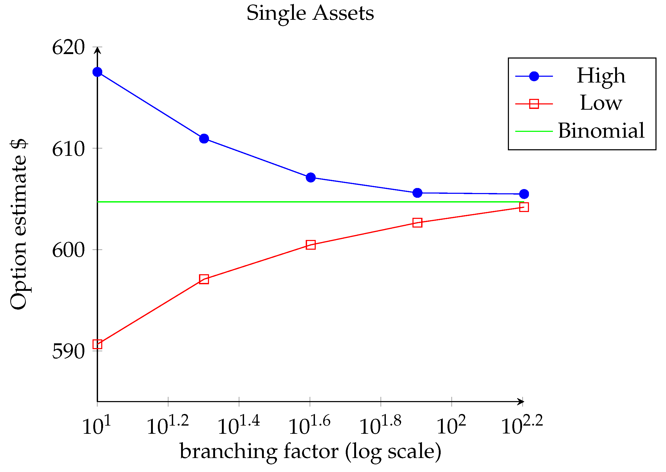
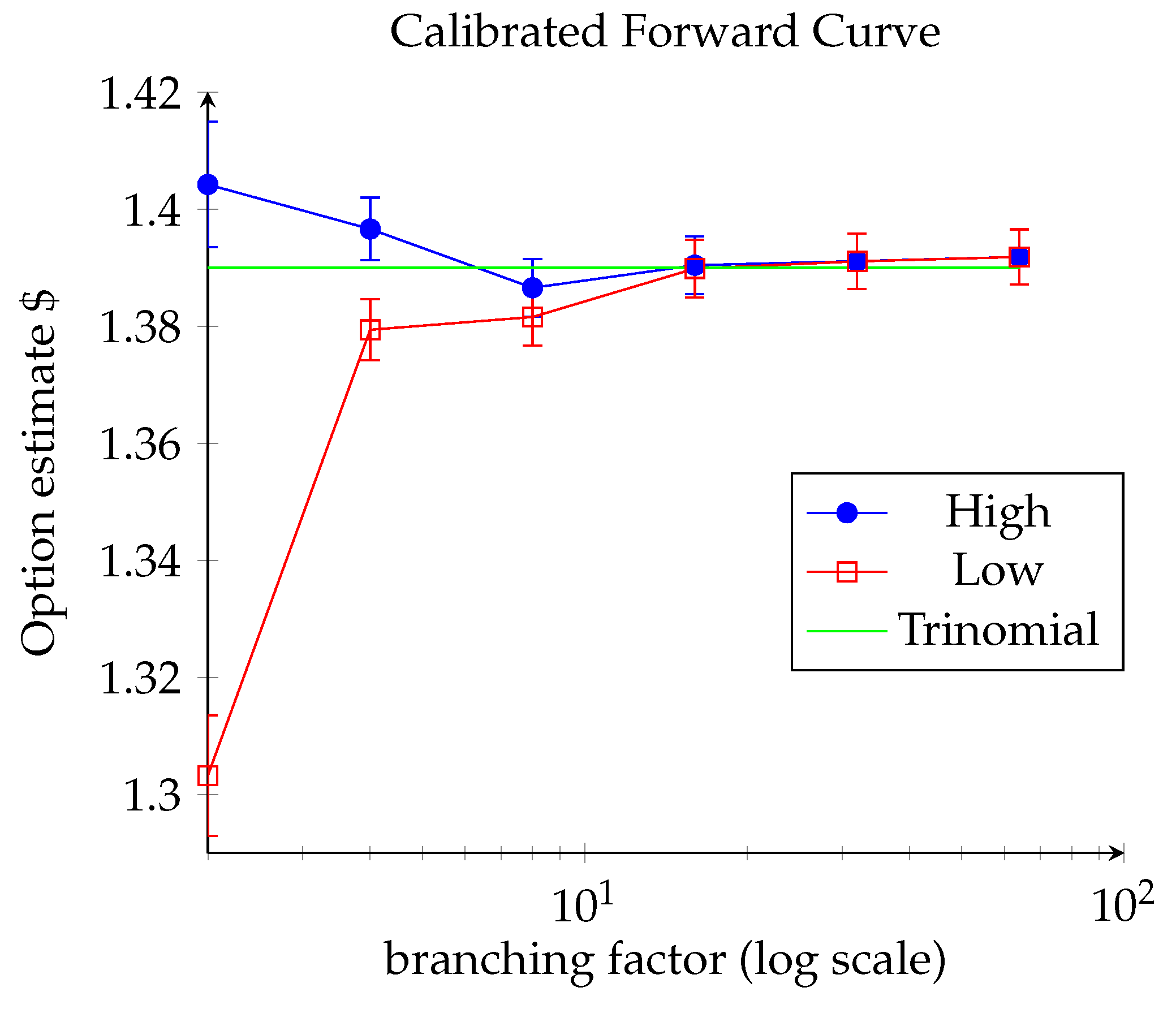
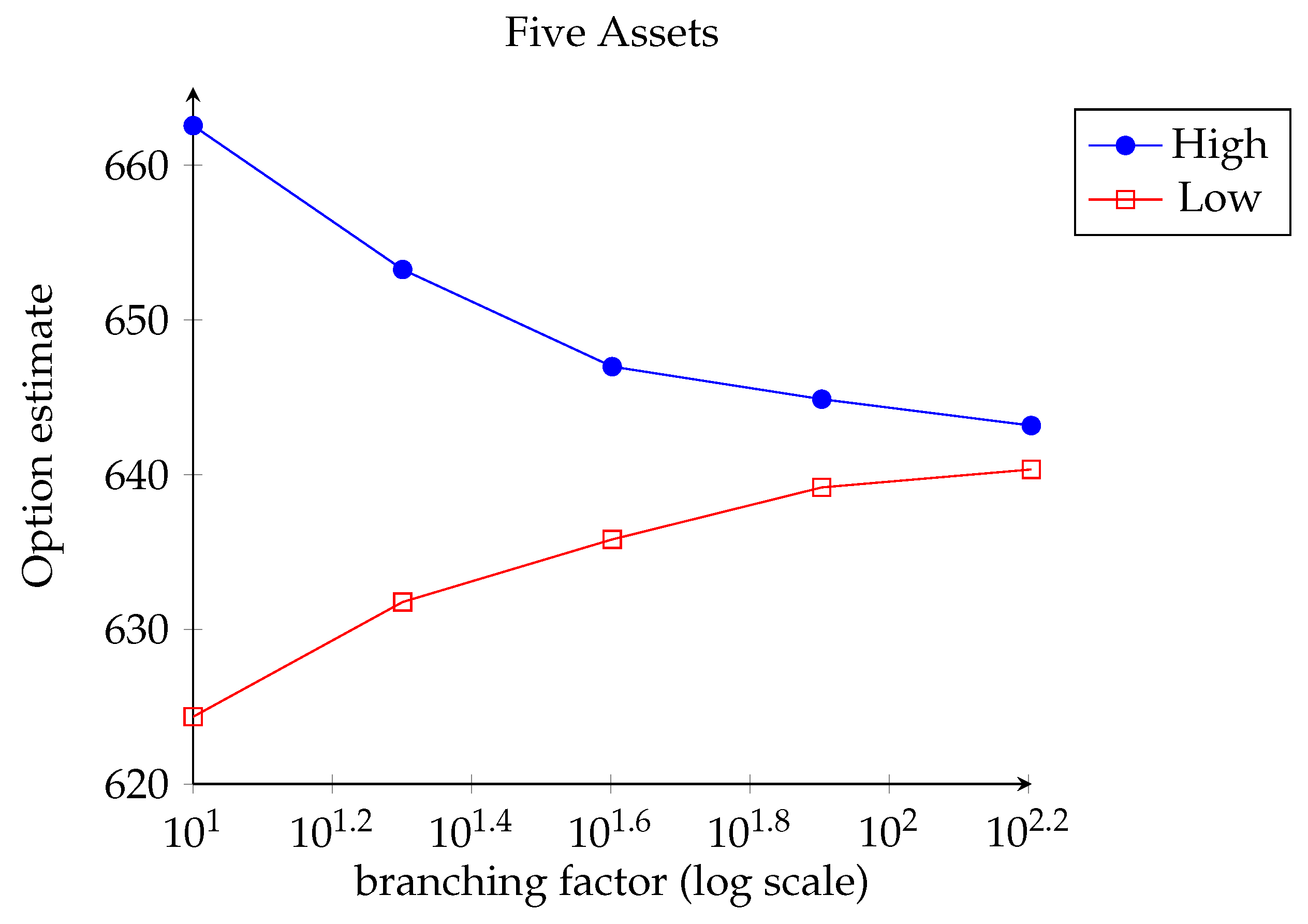
• The high FOST estimator has positive bias.
• The low FOST estimator has negative bias.
• On any given realization the high FOST estimator is at least as big as the low FOST estimator.
• The high and low FOST estimators are asymptotically unbiased.

The remainder of this section provides a literature review. Section 2 describes the Forest of Stochastic Trees estimators in detail; specifies results giving estimator properties (e.g., biasedness and convergence); provides numerical results showing the method is effective at pricing; and supplies discussion on improving computational performance through parallel processing. Section 3 summarizes and concludes the paper. A list of the notation used is given in Appendix A and proofs of the paper’s main theoretical contributions on estimator properties are given in Appendix B.

Literature Review

Multiple exercise options arise in many different areas and the structure of these contracts is typically tailored to particular clients/needs, in contrast to standardized derivatives such as interest rate swaps and exchange-traded commodity futures. A non-exhaustive list of examples of MEOs include (i) tolling agreements used in the steel Kim et al. (2019) and electricity Deng and Oren (2006) sectors; (ii) chooser flexible caps which are exotic interest rate derivatives Meinshausen and Hambly (2004); (iii) valuation and control of energy production and storage facilities Chen and Forsyth (2007); Ludkovski and Carmona (2010); Thompson et al. (2009); and (iv) swing options Calvo-Garrido et al. (2017); Jaillet et al. (2004); Lari et al. (2001); Wilhelm and Winter (2008).

Valuation methods for MEOs are extensions of those used for American-style options. There are continuous-time solutions to both the American-style and multiple exercise option valuation problems; these are computed by solving a system of Hamilton–Jacobi–Bellman quasi-variational inequalities Korn et al. (2005). These methods give more accurate and stable price and sensitivity estimates than those computed using simpler tools (e.g., trees). However, these methods are quite complex mathematically and break down in higher dimensions.

In this article, we focus on the mathematically simpler time-discretized version of the valuation problem. Discrete-time tree-based methods for valuing American-style options Cox et al. (1979) have been extended to MEOs via the Forest of Trees Jaillet et al. (2004); Lari et al. (2001). Techniques for pricing American-style options using solutions of PDEs have been modified to MEOs Calvo-Garrido et al. (2017); Chen and Forsyth (2007); Thompson et al. (2009); Wilhelm and Winter (2008). These methods for MEOs inherit properties similar to the corresponding methods for single-exercise options. One crucial property is that these methods fail as the dimensionality of the problem increases.

Monte Carlo is the obvious tool to overcome the curse of dimensionality, as the rate of convergence of Monte Carlo estimators is independent of the dimension. Tilley (1993) was the first to show that the forward-in-time Monte Carlo approach could be used to solve the backward-in-time dynamic programming problem arising from valuation of an American-style option. Since this seminal paper, numerous other methods for the Monte Carlo valuation of American style options have appeared. These include methods that attempt to parameterize the exercise region Barraquand and Martineau (1995) and those that discretize the state space Bally et al. (2005). Methods that parameterize the early-exercise region have been extended to value multiple exercise options by parameterizing the set of exercise level curves Ibán̎ez (1996). Similarly state space aggregation methods have been used for multiple exercise option valuation Ben Latifa et al. (2016). These approaches, however, also suffer from the curse of dimensionality and do not easily generalize to arbitrary payoffs and underlying price processes.

Monte Carlo methods that do not break down with the dimensionality and that accommodate general payoff and price processes include those that solve the optimal stopping-time problem through estimation of the hold or continuation value. These include the stochastic tree and mesh techniques of Broadie and Glasserman (1997, 2004) and the regression-based approach first appearing in Carriere (1996) and then subsequently generalized in Longstaff and Schwartz (2001). For each of these valuation techniques, high- and low-biased estimators are easily generated, along with a hybrid interleaving estimator that has properties of both. Duality-based methods solve the optimal control problem in the dual space by approximating an optimal martingale, typically by regression Andersen and Broadie (2004); Haugh and Kogan (2004).

Least-squares Monte Carlo has been modified for the pricing of swing options in Barrera et al. (2006); Meinshausen and Hambly (2004), respectively. Although increased dimensionality does not decrease the performance of these methods, they suffer from other drawbacks. In least-squares Monte Carlo methods one must select a set of basis functions on which to run regressions to estimate continuation values. In general only a complete (infinite) set of basis functions results in continuation value estimators that are consistent for the true option value. In practice, of course, a finite set of basis functions is used and introduces an approximation error. Continuation value estimators are consistent for the true approximation value and not the true option value Clement et al. (2001); Stentoft (2004).

Duality methods have been extended to MEOs Bender (2011); Chandramouli and Haugh (2012); Gyurko et al. (2015); Meinshausen and Hambly (2004). Duality methods rely on having a sub-optimal exercise policy that produces a low-biased estimate from which the solution to the dual problem can be approximated to yield a high-biased estimate. Typically regression-based methods are used to estimate the sub-optimal exercise policy Chandramouli and Haugh (2012); Gyurko et al. (2015); Meinshausen and Hambly (2004) implying the above noted issues of least-squares Monte Carlo persist when pricing MEOs. Policy iteration methods such as Bender (2011), yield approximations of the time-0 value at each iteration of the dynamic program. As with the pricing of American-style options this method is advantageous because it removes the requirement to calculate nested conditional expectations prior to the time-0 value being approximated.

The stochastic mesh of Broadie and Glasserman (2004) has been extended to MEOs via the Forest of Stochastic Meshes (FOSM) Marshall (2012); Marshall and Reesor (2011). High and low biased FOSM estimators are derived Marshall and Reesor (2011) and their properties shown Marshall (2012), similar to the work presented here for the Forest of Stochastic Trees estimators.

2. Results

We consider the valuation of multiple exercise options as a stochastic optimal control problem with three relevant state variables—the underlying variable (S), number of exercise rights remaining ($\mathcal{N}$), and usage level (U) assuming some volume control. At each exercise opportunity and given ($S,\mathcal{N},U$), the current values of the state variables, the holder must choose between

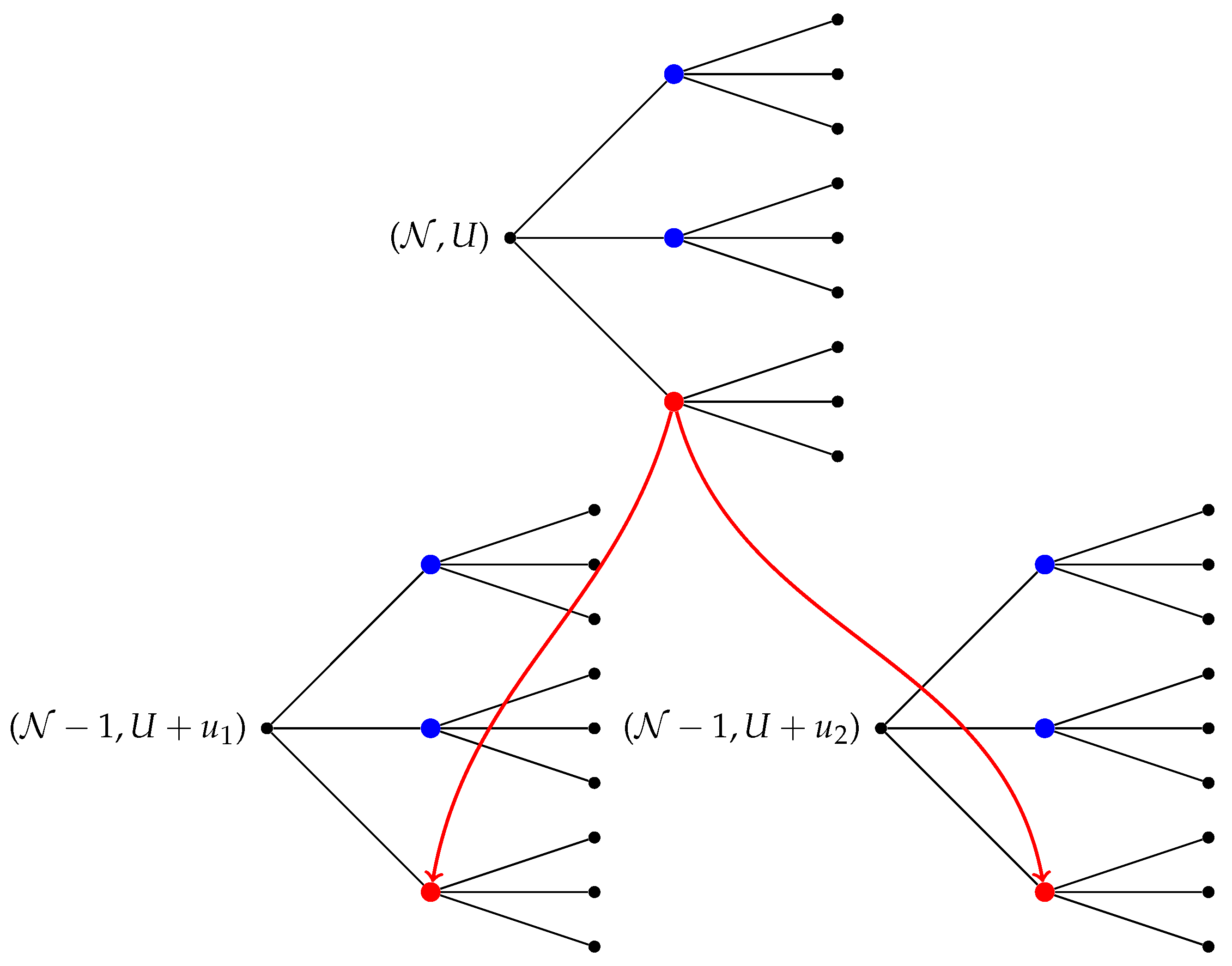
• Exercising u units plus continuing with an option having $\mathcal{N}-1$ remaining exercise rights and usage level $U+u$; and
• Continuing with an option having $\mathcal{N}$ exercise rights and usage level U (i.e., no exercise).

Note that with volume control the payoff from exercising u units changes with u (as does the continuation value of the option). Thus, the holder chooses the value-maximizing u when deciding to exercise. Also note that with $\mathcal{N}=1$ and u constrained to be 1, this is an American-style option.

We work with the time-discretized problem and use dynamic programming to solve for the optimal exercise policy and the corresponding optimal value. In all variables, let the subscript i denote time-$t_i$ and let ${\mathcal{U}}_i$ be the time-$t_i$ set of admissible volume choices which includes the zero volume choice (i.e., hold). The recursive equations for the dynamic program are

$$\begin{array}{cc}\hfill H_i(S_i,{\mathcal{N}}_{i+1},U_{i+1})& =\mathrm{E}\left[B_{i+1}(S_{i+1},{\mathcal{N}}_{i+1},U_{i+1})\right|{\mathcal{Z}}_i]\mathrm{and}\hfill \end{array}$$

(1)

$$\begin{array}{cc}\hfill B_i(S_i,{\mathcal{N}}_i,U_i)& =\underset{u\in {\mathcal{U}}_i}{max}\left[h_i(S_i,{\mathcal{N}}_i,U_i,u)+H_i(S_i,{\mathcal{N}}_i-I_{\{u\ne 0\}},U_i+u)\right],\hfill \end{array}$$

(2)

with the terminal conditions

$$\begin{array}{cc}\hfill H_m(S_m,{\mathcal{N}}_m,U_m)& =\tilde{\varphi }\left(U_m\right)\mathrm{and}\hfill \end{array}$$

(3)

$$\begin{array}{cc}\hfill B_m(S_m,{\mathcal{N}}_m,U_m)& =\underset{u\in {\mathcal{U}}_m}{max}\left[h_m(S_m,{\mathcal{N}}_m,U_m,u)+H_m(S_m,{\mathcal{N}}_m-I_{\{u\ne 0\}},U_m+u)\right],\hfill \end{array}$$

(4)

where $H_i(S,\mathcal{N},U)$ and $B_i(S,\mathcal{N},U)$ are the time-$t_i$, state-${\mathcal{Z}}_i$ continuation and option values, respectively, $h_i(S,\mathcal{N},U,u)$ is the payoff from exercising u units with $h_i(S,\mathcal{N},U,0)=0$, ${\mathcal{Z}}_i$ is the time-$t_i$ information set generated by the paths of ($S,\mathcal{N},U$), I is an indicator function and $\tilde{\varphi }\left(·\right)$ is a cumulative usage penalty term. Estimator properties and their proofs are given for this multiple exercise option setup. However, the dynamic program and estimator properties can be stated and proven for alternative specifications provided there is a finite number of exercise rights and usage levels. For example, a swing option contract may specify a certain number of up and down swing rights, ${\mathcal{N}}_u$ and ${\mathcal{N}}_d$. An up swing right allows the holder to take more than the baseline amount of the underlying asset while a down swing right allows the holder to take less. Another variation is to allow for multiple rights to be exercised at each opportunity where each right corresponds to a fixed volume amount Bender and Schoenmakers (2006); Meinshausen and Hambly (2004).

2.1. Forest of Stochastic Trees

The FOST generalizes the stochastic tree method for valuing American-style options to the valuation of multiple exercise options and extends the Forest of Trees method to handle a high-dimensional underlying asset. This is done by replacing the binomial/trinomial trees with stochastic trees in the framework of Lari et al. (2001) and Jaillet et al. (2004) hence giving the FOST. The stochastic tree is constructed identically as described in Broadie and Glasserman (1997) and the tree is replicated multiple times, with one replication corresponding to each possible ($\mathcal{N},U$) combination. This is analogous to the Forest of Trees in which the same underlying binomial/trinomial tree is replicated for each possible ($\mathcal{N},U$) combination.

The dynamic program is approximately solved by replacing the continuation values in Equations (1) and (3) with stochastic tree-type estimators. As with the original stochastic tree technique, high- and low-biased option value estimators are constructed by using the analogous high- and low-biased estimators, respectively, on each stochastic tree in the forest. The recursive equations for the high estimator are

$$\begin{array}{cc}\hfill {\widehat{H}}_i({\mathbf{S}}_i^{\mathbf{j}},{\mathcal{N}}_{i+1},U_{i+1})& {\displaystyle =\frac{1}{b}\sum _{k=1}^b{\widehat{V}}_{i+1}({\mathbf{S}}_{i+1}^{\mathbf{k}},{\mathcal{N}}_{t+1},U_{t+1}),and}\hfill \end{array}$$

(5)

$$\begin{array}{cc}\hfill {\widehat{V}}_i({\mathbf{S}}_i^{\mathbf{j}},{\mathcal{N}}_i,U_i)& =\underset{u\in {\mathcal{U}}_i}{max}\left[h_i({\mathbf{S}}_i^{\mathbf{j}},{\mathcal{N}}_i,U_i,u)+{\widehat{H}}_i({\mathbf{S}}_i^{\mathbf{j}},{\mathcal{N}}_i-I_{\{u\ne 0\}},U_i+u)\right],\hfill \end{array}$$

(6)

with the terminal conditions

$$\begin{array}{cc}\hfill {\widehat{V}}_m({\mathbf{S}}_m^{\mathbf{j}},{\mathcal{N}}_m,U_m)& =\underset{u\in {\mathcal{U}}_m}{max}\left[h_m({\mathbf{S}}_m^{\mathbf{j}},{\mathcal{N}}_m,U_m,u)+\tilde{\varphi }\left(U_m+u\right)\right],\hfill \end{array}$$

(7)

where ${\widehat{H}}_i(\mathbf{S},\mathcal{N},U)$ and ${\widehat{V}}_i(\mathbf{S},\mathcal{N},U)$ are the time-$t_i$, state-${\mathcal{Z}}_i$ continuation and option value estimators, respectively, $h_i(\mathbf{S},\mathcal{N},U,u)$ (with $h_i(\mathbf{S},\mathcal{N},U,0)=0$) is the time-$t_i$, state-${\mathcal{Z}}_i$ payoff from exercising u units, b is the branching factor, I is an indicator function and $\tilde{\varphi }\left(U_m+u\right)$ is a global usage penalty term. The superscript $\mathbf{j}=\{j_0,j_1,\dots ,j_i\}$ indicates the specific node within a given stochastic tree and $\mathbf{k}=\{\mathbf{j},k\}$.

Figure 1 is a diagram of a section of a Forest of Stochastic Trees with two volume choices, $u_1$ and $u_2$. It illustrates the nodes in the forest which need to be considered when making an exercise decision given state ($\mathcal{N},U$). The three choices are no exercise, exercise $u_1$ units, and exercise $u_2$ units.

The low estimator is similarly defined using the low estimator on each stochastic tree via the dynamic program,

$$\begin{array}{cc}\hfill {\widehat{g}}_{il}({\mathbf{S}}_i^{\mathbf{j}},{\mathcal{N}}_i,U_i,u)& {\displaystyle =h_i\left({\mathbf{S}}_i^{\mathbf{j}},{\mathcal{N}}_i,U_i,u\right)+\frac{1}{b-1}\underset{k\ne l}{\sum _{k=1}^b}{\widehat{v}}_{i+1}({\mathbf{S}}_{i+1}^{\mathbf{k}},{\mathcal{N}}_i-I_{\{u\ne 0\}},U_i+u),}\hfill \end{array}$$

(8)

$$\begin{array}{cc}\hfill {\widehat{H}}_{il}({\mathbf{S}}_i^{\mathbf{j}},{\mathcal{N}}_i,U_i)& =\underset{u\in {\mathcal{U}}_i}{max}\left[{\widehat{g}}_{il}({\mathbf{S}}_i^{\mathbf{j}},{\mathcal{N}}_i-I_{\{u\ne 0\}},U_i+u)\right],\hfill \end{array}$$

(9)

$$\begin{array}{cc}\hfill {\widehat{v}}_{il}({\mathbf{S}}_i^{\mathbf{j}},{\mathcal{N}}_i,U_i)& =h_i({\mathbf{S}}_i^{\mathbf{j}},{\mathcal{N}}_i,U_i,{\widehat{u}}^{*})+{\widehat{v}}_{i+1}({\mathbf{S}}_{i+1}^{\mathbf{l}},{\mathcal{N}}_i-I_{\{u^{*}\ne 0\}},U_i+{\widehat{u}}^{*}),\mathrm{and}\hfill \end{array}$$

(10)

$$\begin{array}{cc}\hfill {\widehat{v}}_i({\mathbf{S}}_i^{\mathbf{j}},{\mathcal{N}}_i,U_i)& =\frac{1}{b}\sum _{l=1}^b{\widehat{v}}_{il}({\mathbf{S}}_i^{\mathbf{j}},N_i,U_i)\hfill \end{array}$$

(11)

where ${\widehat{H}}_{il}({\mathbf{X}}_i^j,{\mathcal{N}}_i,U_i)$ is the $l$-th leave-one-out hold value estimator and ${\widehat{u}}^{*}$ is the estimated optimal exercise amount which depends on i and l. The terminal conditions associated with this dynamic programming scheme are,

$$\begin{array}{cc}\hfill {\widehat{v}}_m({\mathbf{S}}_m^{\mathbf{j}},{\mathcal{N}}_m,U_m)& =\underset{u\in {\mathcal{U}}_m}{max}\left[h_m({\mathbf{S}}_m^j,{\mathcal{N}}_m,U_m,u)+\tilde{\varphi }\left(U_m+u\right)\right],\hfill \end{array}$$

(12)

where $\tilde{\varphi }\left(U_m+u\right)$ is a cumulative usage penalty term.

2.2. Estimator Bias

In order to justify using the high- and low-biased estimators to construct upper and lower option price bounds, respectively, we prove that the high estimator is always positively biased and that the low estimator is always negatively biased. In addition we include a comparison of the estimators which orders their values on any realization of the simulated forest.

The theorems that follow are direct extensions of those in Broadie and Glasserman (1997). Below, the branching factor, b, appears as an argument in the estimators. For example, ${\widehat{V}}_0(b,{\mathbf{S}}_0,{\mathcal{N}}_0,U_0)$ refers to the time-0, state-${\mathcal{Z}}_0$ high-biased estimator with a stochastic tree branching factor of b. This argument has been suppressed to this point for convenience. We begin with the theorem regarding the bias of the high estimator.

Theorem 1.

(High estimator bias) The high estimator is biased high, i.e.,

$$\mathrm{E}\left[{\widehat{V}}_0\left(b,{\mathbf{S}}_0,{\mathcal{N}}_0,U_0\right)\right]\ge B_0\left({\mathbf{S}}_0,{\mathcal{N}}_0,U_0\right)$$

(13)

for all b.

Similarly, the result stating the bias of the low estimator follows.

Theorem 2.

(Low estimator bias) The low estimator is biased low, i.e.,

$$\mathrm{E}\left[{\widehat{v}}_0\left(b,{\mathbf{S}}_0,{\mathcal{N}}_0,U_0\right)\right]\le B_0\left({\mathbf{S}}_0,{\mathcal{N}}_0,U_0\right)$$

(14)

for all b.

Finally, an ordering result for the high and low estimators is stated in Theorem 3.

Theorem 3.

(Comparison of Estimators) On every realization of the forest the low estimator is less than or equal to the high estimator. That is,

$${\widehat{v}}_i\left(b,{\mathbf{S}}_i^{\mathbf{j}},{\mathcal{N}}_i,U_i\right)\le {\widehat{V}}_i\left(b,{\mathbf{S}}_i^{\mathbf{j}},{\mathcal{N}}_i,U_i\right)$$

(15)

with probability one for all $\mathbf{j}$, i.

Theorems 1–3 are proven in Appendix B.

2.3. Estimator Convergence

An advantage of the stochastic tree method over some other MC valuation methods is that its estimators are consistent to the true option value. This property also holds for the FOST estimators. In this section we state two theorems—one for the consistency of the high estimator, and the other for the consistency of the low estimator. Here convergence is in probability to the true option value and as above the argument b that appears with the estimators refers to an arbitrary branching factor size of b with convergence being shown as $b\to \infty$. Before stating the result, define ${\overline{V}}_0\left(b,{\mathbf{S}}_0,{\mathcal{N}}_0,U_0\right)$ as the average of R independent replications of ${\widehat{V}}_0\left(b,{\mathbf{S}}_0,{\mathcal{N}}_0,U_0\right)$.

Theorem 4.

(High estimator convergence) Suppose $\mathrm{E}\left[{\left|h_i\left({\mathbf{S}}_i,{\mathcal{N}}_i,U_i\right)\right|}^{p^{\prime }}\right]<\infty$, for all $t_i$, and some $p^{\prime }>1$. Then ${\overline{V}}_0\left(b,{\mathbf{S}}_0,{\mathcal{N}}_0,U_0\right)$ converges to $B_0\left({\mathbf{S}}_0,{\mathcal{N}}_0,U_0\right)$ in p-norm for any $0<p<p^{\prime }$ as $b\to \infty$. This holds for an arbitrary number of repeated valuations of the forest, R. In particular ${\overline{V}}_0\left(b,{\mathbf{S}}_0,{\mathcal{N}}_0,U_0\right)$ converges to $B_0\left({\mathbf{S}}_0,{\mathcal{N}}_0,U_0\right)$ in probability and is thus a consistent estimator of the option value.

This results implies that

$$\mathrm{E}\left[{\widehat{V}}_0\left(b,{\mathbf{S}}_0,{\mathcal{N}}_0,U_0\right)\right]\to B_0\left({\mathbf{S}}_0,{\mathcal{N}}_0,U_0\right)$$

(16)

as $b\to \infty$. Hence the estimator is asymptotically unbiased.

Theorem 5.

(Low estimator convergence) Suppose that,

$$\begin{array}{cc}\hfill & \mathrm{P}\left[h_i\left({\mathbf{S}}_i,{\mathcal{N}}_i,U_i,u^1\right)+H_i\left({\mathbf{S}}_i,{\mathcal{N}}_i-I_{\{u^1\ne 0\}},U_i+u^1\right)\right.\hfill \\ \hfill & \ne h_i\left.\left({\mathbf{S}}_i,{\mathcal{N}}_i,U_i,u^2\right)+H_i\left({\mathbf{S}}_i,{\mathcal{N}}_i-I_{\{u^2\ne 0\}},U_i=u^2\right)\right]=1,\hfill \end{array}$$

for $u^1,u^2\in {\mathcal{U}}_i$, $u^1\ne u^2$ and all i. Then Theorem 4 also holds for the low estimator.

The additional condition imposed in Theorem 5 is analogous to that used in Theorem 3 of Broadie and Glasserman (1997). This condition says that, with probability one, the optimal exercise policy is never indifferent between the choices of volumes to exercise (including $u=0$). As in Broadie and Glasserman (1997) imposing this condition simplifies the analysis of the estimator. Theorems 4 and 5 are proven in Appendix B.

2.4. Numerical Results

Pricing swing contracts involves a large number of parameters and in this section we provide some results which illustrate the validity of our method across a variety of specifications. We assume that the underlying assets follow a risk neutral stochastic process, there are no transaction costs and other than penalties, there are no other constraints considered. We also assume a constant risk free rate of interest and the volatilities of all assets are known constant functions of time.

The option swing rights may be exercised at discrete times up to and including expiry and the volume choices given are in discrete amounts. That is, anytime the holder chooses to exercise a right, they must choose from a finite list of possible volume amounts. The rationale behind allowing all time steps to be exercise opportunities is the exponential growth in computational time caused by adding intermediate non-exercise times. However, the method can easily be modified to incorporate these extra time steps. As previously mentioned penalties can be implemented globally and are based on the net volume exercised during the contract.

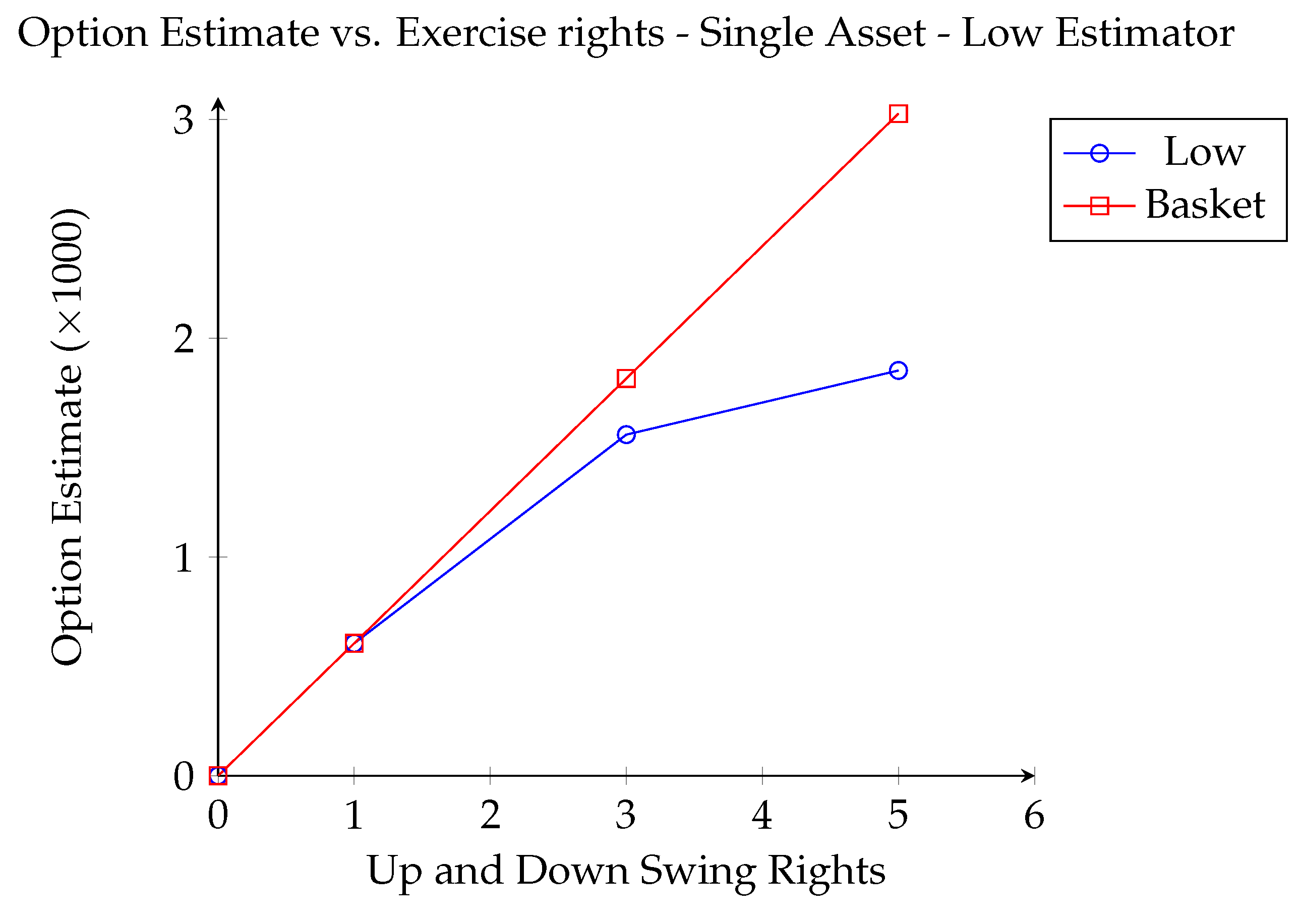
2.4.1. Single Dimension

Beginning with the one dimensional case, we have based our simulations on an underlying asset with a risk neutralized price process that satisfies the following stochastic differential equation,

$$d{S}_i=S_i\left[\left(r-\delta \right)dt+\sigma d{Z}_i\right].$$

(17)

In this equation, r is the riskless interest rate, $Z_i$ is a standard Brownian motion process, $\sigma$ is a constant volatility parameter and the underlying asset itself pays a continuous dividend yield $\delta$. The parameter values for the underlying asset are specified as $r=0.05$, $\delta =0.1$, and $\sigma =0.2$.

The swing options considered have both up and down swing rights and the payoff upon exercise is

$$u\times max\left[max\left(S-K_u,0\right),max\left(K_d-S,0\right),0\right],$$

(18)

where u is the volume exercised, S is the price of the underlying asset at the exercise time, and $K_u$ and $K_d$ are the up and down swing strike prices, respectively. For the examples considered here, we set $K_u=K_d=K$ which simplifies the payoff function to

$$u\times max\left(S-K,K-S\right).$$

(19)

For all examples in Section 2.4.1 the option expiry is 3.0 years and the options have both up and down swing rights with strike prices $K_u=K_d=40.0$, respectively. In examples where the holder controls the amount exercised, a list of volume choices is given. The volume choices are consecutive integer multiples of a base amount and the up swing and down swing volumes have the same magnitude. For comparison purposes the results in this subsection include a binomial value which is calculated using the Forest of Trees Lari et al. (2001).

All simulations in this subsection were completed on the SHARCNet cluster Whale. Whale is located at the University of Waterloo and consists of Opteron 2.2 GHz processors (four per node) with a Gigabit Ethernet interconnect. Timing results listed below are given in total cpu time accumulated which is approximately equal to (program runtime) × (number of processors used).

Example 1.

(Illustration of Bias and Convergence) The swing option in this example has one up and one down swing right, three exercise opportunities, exercise volume of 60 units of the underlying and there is no penalty. The initial price is USD 40. Here we illustrate the effect of the branching factor b on the value estimates. Specifically, we perform R repeated valuations of the FOST with a branching factor of b and hold the total sample size fixed using the relation $R=32,000\left(\frac{10}{b}\right)$. Figure 2 plots the FOST estimates versus branching factor (the estimates are the averages of the R repeated valuations). Taking the Binomial estimate as the true option value, it is clear that the high estimator overestimates the true price while the low estimator underestimates the true price. Furthermore, as the branching factor increases, the high estimator decreases and the low estimator increases to the true option price, clearly illustrating estimator convergence. Estimator standard errors are approximately 0.07% of estimator value.

Example 2.

(Effect of Usage Penalty and Initial Asset Price) In this example, the option has two up and two down swing rights and, upon exercise there are three volume choices—20, 40 and 60 units of the asset. Should the final net volume exercised exceed 90 units or be below −90 units a penalty is imposed. The penalty is calculated by multiplying the terminal asset price by ten times the excess usage above 90 units or below −90 units. To see the effect of the penalty on option value, we also turn the penalty term off and value the corresponding option with no penalty. The initial asset value ranges from USD 20 to USD 60 in steps of USD 10. There are $m=5$ exercise opportunities and we use a branching factor of $b=20$ with $R=4000$ repeated valuations.

The pricing results are presented in

Table 2. Swing option values as a function of initial asset price and usage penalty with a single underlying asset. Parameter values used are ${\mathcal{N}}_u={\mathcal{N}}_d=2$, ${\mathcal{U}}_i=\{20,40,60\}$, $b=20$, $R=4000$, $m=5$, $U_{min}=-90$, and $U_{max}=90$.

${\mathit{S}}_0$	Penalty	High	Error	Low	Error	Binomial
60	ON	2271.153	1.418	2240.319	1.378	2259.845
	OFF	2422.781	1.576	2392.872	1.523	2411.844
50	ON	1445.468	0.844	1408.843	0.904	1429.645
	OFF	1542.053	0.978	1503.963	0.980	1526.055
40	ON	1018.104	0.859	968.793	1.044	989.651
	OFF	1156.591	0.911	1134.093	0.903	1145.801
30	ON	1345.556	1.205	1309.214	1.280	1326.266
	OFF	1562.347	1.316	1532.854	1.343	1546.055
20	ON	2189.531	0.905	2147.623	1.018	2157.976
	OFF	2443.877	0.924	2402.192	1.034	2412.354

. In each row of the table, we see that the high and low estimators bound the true price. Unsurprisingly, imposing a penalty on the cumulative volume reduces the option value. Furthermore, as the initial stock price increases, the increase in an up swing right’s value is more than the decrease in a down swing right’s value. The opposite is true as the initial stock price decreases. The end result is that as the initial stock price moves away from being at-the-money, the option value increases.

The average computing time per row (not including the binomial forest valuation) was 5.6 h for the cases with usage penalty and was 1.1 h without usage penalty. The reduction in runtime for the case with no penalty can be described as follows. If there are no constraints (e.g., penalty, storage) on the option holder then upon exercise it is always optimal to choose the maximum amount. Therefore with no penalty this option is equivalent to that of an otherwise identical swing option with no volume choices and an exercise volume of 60 units. The latter has fewer trees in its forest and is therefore quicker to evaluate. In Table 2 we have chosen to exploit this as a convenient way to save computational time. For the binomial method run times were on the order of a few seconds.

Example 3.

(Effect of Number of Exercise Rights) In this example we illustrate that the option value increases with the number of exercise rights and compare the swing option value with that of a corresponding basket of American options. The option has $m=5$ exercise opportunities, an exercise volume of 60 units, and there is no usage penalty. Additionally, we set the initial price to $S_0=40$ and use a branching factor of $b=20$ with $R=4000$ repeated valuations. We consider options having an equal number of up and down swing rights.

Table 3. Swing option values as a function of the number of exercise rights with a single underlying asset. Parameter values used are exercise volume of 60 units, $S_0=40$, $b=20$, $R=4000$, $m=5$, and no usage penalty.

${\mathcal{N}}_{\mathit{u}}={\mathcal{N}}_{\mathit{d}}$	High	Error	Low	Error	Binomial
1	630.054	0.449	605.394	0.453	617.832
3	1573.237	1.449	1559.517	1.437	1567.344
5	1852.788	2.128	1852.788	2.128	1852.627

gives the option price estimates for ${\mathcal{N}}_u={\mathcal{N}}_d=1,3,5$ along with prices computed using the Forest of Trees. First notice that the high and low estimates bound the true option from the binomial model. Next note that with ${\mathcal{N}}_u={\mathcal{N}}_d=5$ exercise rights, the high and low estimates are exactly the same. In this case the number of exercise opportunities is equal to the numbers of up and down swing rights and since the up and down swing strikes are equal, exactly one of these rights will be exercised at each opportunity (see Equation (19)). This makes both the exercise payoff and the continuation value estimates exactly the same at all times and along all branches for both the low and high estimators, yielding identical prices.

Second, the option value increases with the number of swing rights. However, the price increases by a factor that is less than the increase in the number of swing rights. For example, when the number rights increases by a factor of 3 (e.g., going from ${\mathcal{N}}_u={\mathcal{N}}_d=1$ to ${\mathcal{N}}_u={\mathcal{N}}_d=3$) the option value increases by a factor of 2.5 and when the number of rights increases by a factor of $\frac{5}{3}$ (e.g., going from ${\mathcal{N}}_u={\mathcal{N}}_d=3$ to ${\mathcal{N}}_u={\mathcal{N}}_d=5$), the option value increases by a factor of 1.2. This result matches with the intuition that a swing option with a given number of rights is less valuable than a basket of American put and call options with otherwise identical parameters and $K_d\le K_u$.

For the case of one up and one down swing right the basket of American options would contain a single call corresponding to the up swing right and a single put corresponding to the down swing right, with equal strike prices for the call and put. Changing the number of up and down swing rights invokes a change in the corresponding number of call and put options in the basket. Figure 3 shows a comparison between the values of a basket of American options and a swing option with a comparable number of exercise rights. The value of the basket is linear in the number of exercise rights and the swing option value is below the value of the corresponding basket when the number of rights is greater than one. This follows from the restriction that only one swing right may be exercised at any exercise opportunity whereas all American options of a particular type could be exercised at a given time. In the case of one up and one down right the two are equal since it would never be optimal to exercise both the put and call style rights at the same time. As the number of rights increases, the difference in values increases due to the swing option restriction allowing only a single right to be exercises at each opportunity. The low-biased estimator is used for both the basket and swing option values in Figure 3.

2.4.2. Calibrated Forward Curve

In this example, we use the trinomial-tree model described in Section 4 of Jaillet et al. (2004) from which price movements are simulated. This model is a 1-factor model with mean reversion that is seasonally adjusted and calibrated to the forward curve. The option we value is Example (a) of Section 4.2 in Jaillet et al. (2004). This option a two up right swing option with each right allowing the holder to take delivery of either 1 or 2 MMBTus of natural gas. We simplify to have four exercise opportunities and 4 months until expiry. Upon exercise the holder gets

$$max\left(U_i\left(A_i{S}_i-K\right),0\right)$$

(20)

where $U_i$ is the volume chosen, $A_i$ is the seasonality factor and $S_i$ is the deseasonalized spot price.

Figure 4 plots the option price estimates, including 95% confidence intervals, against branching factor. The number of repeated valuations used to generate prices with a branching factor of b is $R=\frac{160,000}{b}$. We see that, with a branching factor of only 8, the confidence intervals for the high- and low-biased estimators begin to overlap and quickly become almost indistinguishable for higher branching factors, numerical illustration of both estimators’ consistency. Additionally, the high and low estimators converge to the true price computed using the trinomial model. We note that the serial computational times (for a single FOST valuation) for branching factors of 8 and 32 were approximately 4.5 and 110 s, respectively using a 2.1 Ghz Core 2 Duo processor. The pricing results shown in Figure 4 are consistent with the results in Jaillet et al. (2004) but we note that the valuation method in that publication breaks down in higher dimensions and in cases where the inclusion of more risk factors is desirable.

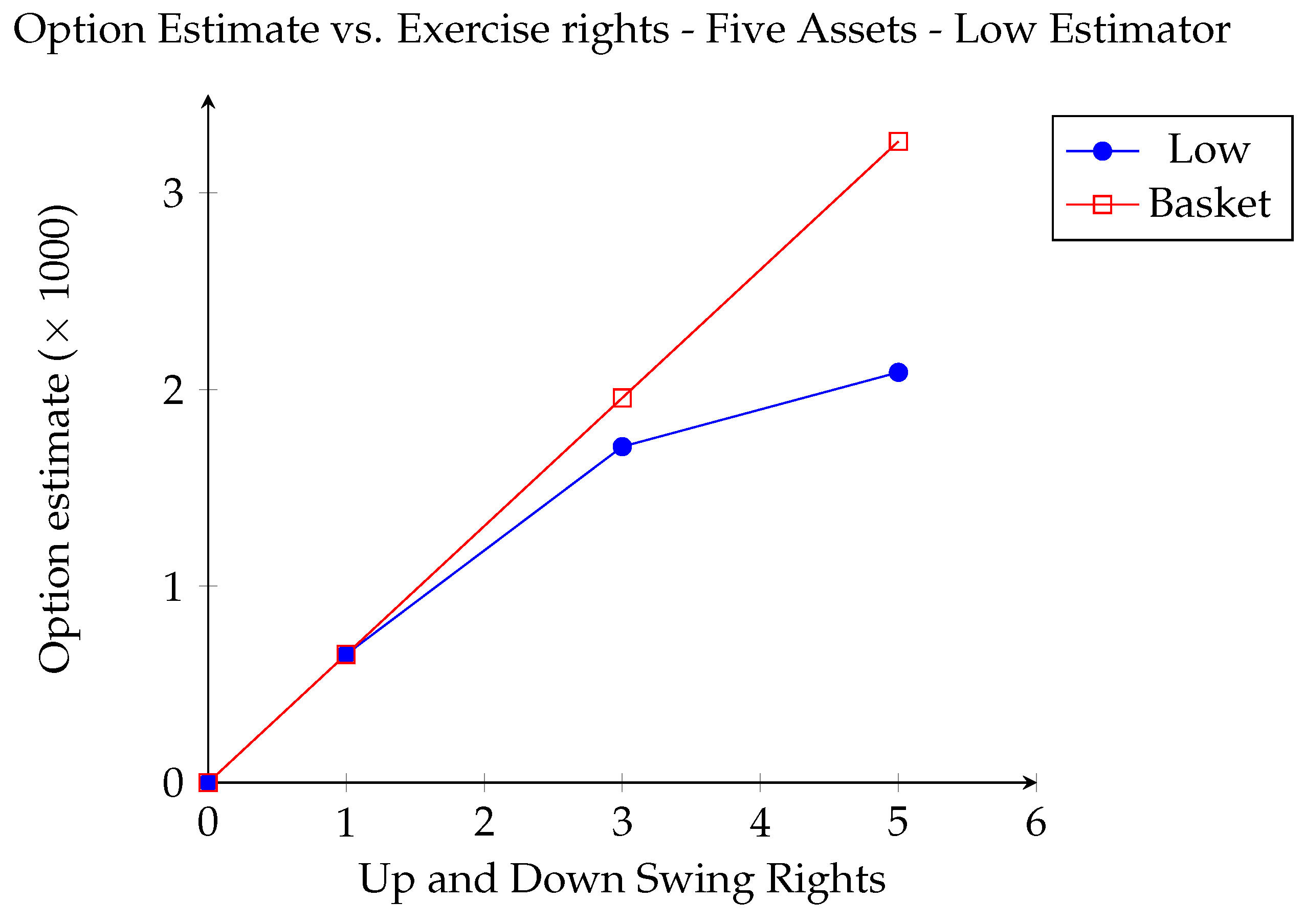
2.4.3. Five Dimensions

Due to the computationally intensive nature of this method it only becomes truly useful in cases where PDE or tree based methods fail. In this subsection we present high-dimensional versions of the examples presented in Section 2.4.1. The asset prices are assumed to follow a risk neutralized correlated geometric Brownian motion described by the stochastic differential equations,

$$d{S}_i^k=S_i^k\left[\left(r-{\delta }^k\right)dt+{\sigma }^{k}d{Z}_i^k\right],k=1,\dots ,d,$$

(21)

where $Z_i^k$ is a standard Brownian motion process and the instantaneous correlation between $Z^k$ and $Z^s$ is ${\rho }^{ks}$. Here the parameter values are specified as $r=0.05$, ${\delta }^k=\delta =0.1$, ${\sigma }^k=\sigma =0.2$ for all k and that ${\rho }^{ks}=0$ for all $k\ne s$. In addition all assets have the same initial value, $S_0$, and we take the number of assets to be $d=5$.

The swing options considered have both up and down swing rights and the payoff upon exercise is

$$u\times max\left[\left(\underset{k=1,\dots ,d}{max}{S}^k-K_u,K_d-\underset{k=1,\dots ,d}{max}{S}^k\right),0\right],$$

(22)

where $S^k$ is the price of the kth underlying asset at the exercise time. This payoff is an extension of the example given in Broadie and Glasserman (1997) and Broadie and Glasserman (2004) for single-exercise American-style options. For the examples considered here, we set $K_u=K_d=K$ which simplifies the payoff function to

$$u\times max\left(\underset{k=1,\dots ,d}{max}{S}^k-K,K-\underset{k=1,\dots ,d}{max}{S}^k\right).$$

(23)

As in Section 2.4.1, the option expiry is 3.0 years and the options have both up and down swing rights with strike prices $K_u=K_d=40.0$, respectively. In examples where the holder controls the amount exercised, a list of volume choices is given. Note that we present results from our FOST methodology without comparisons to other methods as there is no generally accepted benchmark for the examples considered here.

Example 4.

(Illustration of Bias and Convergence) This 5-dimensional example corresponds with Example 1. The swing option has one up and one down swing right, three exercise opportunities, exercise volume of 60 units of the underlying and there is no penalty. The initial price is USD 40. We perform R repeated valuations of the FOST with a branching factor of b and hold the total sample size fixed using the relation $R=32000\left(\frac{10}{b}\right)$. This results in standard errors ≈ 0.09% of option value. Figure 5 plots the FOST estimates versus branching, showing that the high estimator overestimates the option price while the low estimator underestimates the price. Furthermore, as the branching factor increases, the high estimator decreases and the low estimator increases and they appear to be converging to the same value, illustrating estimator convergence. These findings are consistent with those in Example 1.

Example 5.

(Effect of Usage Penalty and Initial Asset Price) This 5-dimensional example corresponds with Example 2, with the option specifications the same as presented there, modulo the adjustment to the payoff function to five dimensions. The pricing results are in

Table 4. Swing option values as a function of moneyness and penalties with a five-dimensional underlying asset. Parameter values used are ${\mathcal{N}}_u={\mathcal{N}}_d=2$, ${\mathcal{U}}_i=\{20,40,60\}$, $b=20$, $R=4000$, $m=5$, $U_{min}=-90$, and $U_{max}=90$.

${\mathit{S}}_0$	Penalty	High	Error	Low	Error
60	ON	3577.280	2.864	3517.297	2.845
	OFF	3832.050	2.286	3772.123	2.856
50	ON	2246.657	2.280	2197.957	2.259
	OFF	2479.081	2.341	2431.065	2.318
40	ON	1221.847	1.595	1189.610	1.564
	OFF	1257.171	1.499	1226.370	1.467
30	ON	1105.831	0.453	1087.851	0.447
	OFF	1209.179	0.393	1196.255	0.391
20	ON	1937.615	0.445	1930.860	0.472
	OFF	2177.194	0.489	2177.031	0.513

. The effects of a usage penalty and initial stock price are qualitatively the same compared with the 1-dimensional results. We note that the option value estimates in this example are higher than those in Example 2 due to the payoffs depending on the maximum of the five asset prices. The computing times for the 5-dimensional case are similar to those for the 1-dimensional asset.

Example 6.

(Effect of Number of Exercise Rights) This 5-dimensional example corresponds with Example 3, with the option specifications the same as presented there, modulo the adjustment to the payoff function to five dimensions. The results are given in

Table 5. Swing option values as a function of the number of exercise rights with a five-dimensional underlying asset. Parameter values used are base volume = 60 units, $S_0=40$, $b=20$, $R=4000$, $m=5$, and no usage penalty.

${\mathcal{N}}_{\mathit{u}}={\mathcal{N}}_{\mathit{d}}$	High	Error	Low	Error
1	683.144	0.741	652.481	0.721
3	1728.947	2.279	1709.497	2.248
5	2087.495	3.114	2087.495	3.114

and Figure 6. The results, intuition, and interpretation are qualitatively the same as the 1-dimensional results.

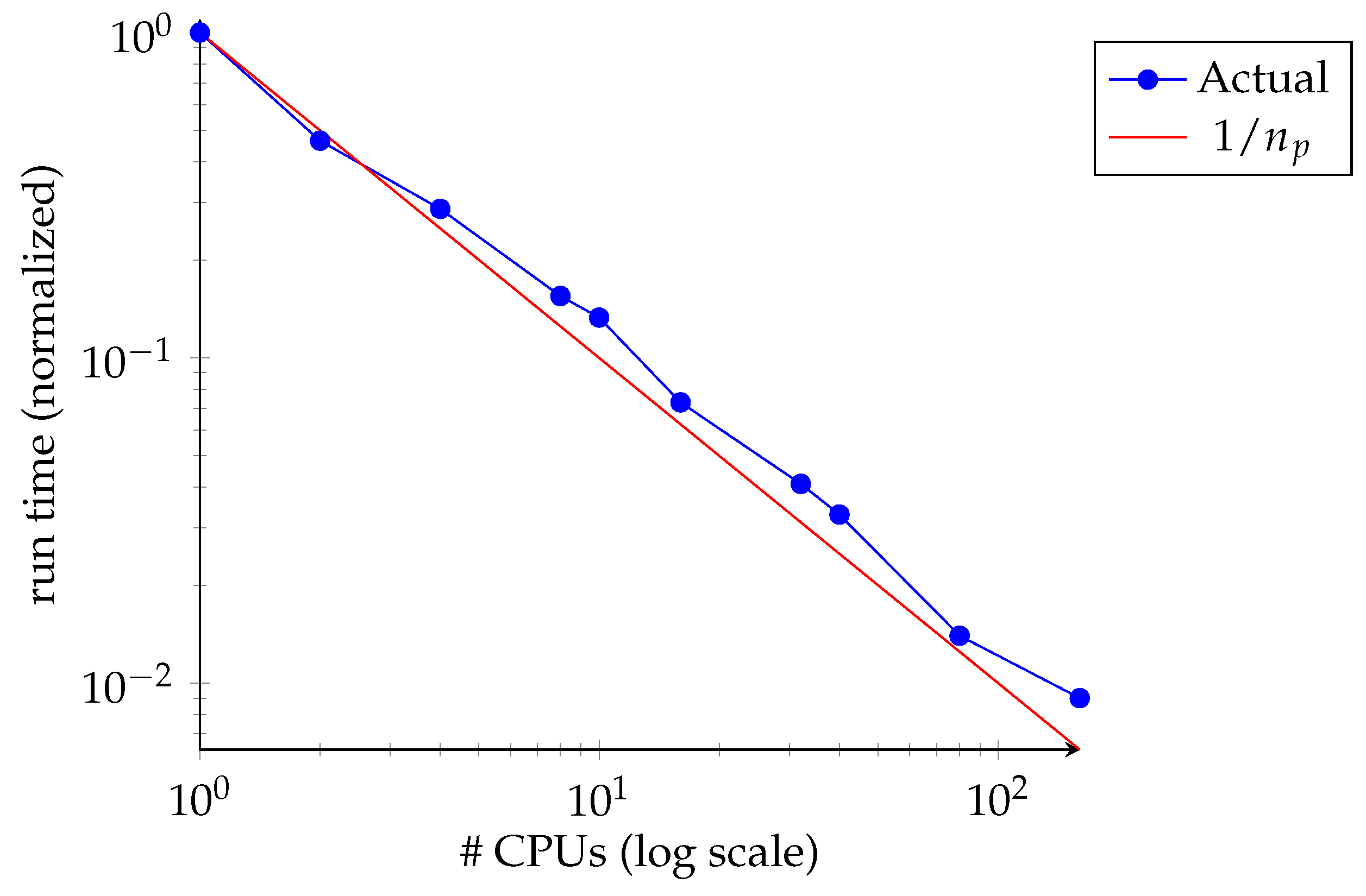
2.5. Algorithmic Enhancement via Parallel Processing

One method for enhancing the computational efficiency of this algorithm is by taking advantage of multi-processor computing techniques. The simplest and most obvious implementation would be to parallelize across repeated valuations of the forest resulting in serial farming of the repeated valuations. Since each repeated valuation results in an iid random value for the option estimate, the generation of all the results may be completed independently of one another, removing the need for communication between processors. This method is simple and effective. However we state here without numerical evidence that it results in a near perfect speed up without the need for expensive interconnections. With this method the minimum run time that can be produced is determined by the number of processors available, the number of repeated valuations necessary for the desired accuracy and the run time of a single forest.

A variation on the aforementioned parallel implementation is to parallelize the FOST computations internally within the forest. In the results shown in Figure 7 the FOST algorithm has been modified so that the computation of the individual trees within the forest is done using multiple processors. Here we have begun the parallelization after the first time step by dividing up the computation of the remaining subtrees across different processors. Upon completion, the results are gathered and the option value at the initial time step is determined. In Figure 7 we see that this method results in a near perfect speed up due to the small ratio of communication time versus computational time. This implementation may be combined with serial farming resulting in further computational time efficiency. This is discussed more fully in Marshall et al. (2011).

In Figure 7 the swing option is identical one in Example 4 and pricing is done with a branching factor $b=160$. The computational times were generated using the SHARCNET cluster Hound which comprises 2.2 GHz Opteron processors with 4 GB per core and Infini-Band interconnections. Run times are normalized to the run time of a single processor.

3. Discussion and Conclusion

The FOST can be thought of as generalizations of two existing pricing methodologies. First, it generalizes the Forest of Trees method to a high-dimensional underlying. Second, it generalizes the Stochastic Tree pricing method for single-exercise right options to multiple exercise rights. We construct high and low FOST estimators analogous to those defined for the Stochastic Tree. We prove properties regarding FOST estimator bias, ordering, and convergence and present numerical results as illustrations.

In related work, we have replaced the binomial/trinomial trees in the Forest of Trees method with Stochastic Meshes Broadie and Glasserman (2004), creating the Forest of Stochastic Meshes Marshall and Reesor (2011). This avoids the exponential growth in computing time with the number of exercise opportunities experienced by the FOST. Another avenue of future work involves algorithmic enhancement. In Section 2.5 we discussed the use of parallel processing to reduce computing time. Two alternatives to this are variance reduction and bias reduction. There are some standard variance reduction methods (e.g., antithetic variates, control variates) that could be used to produce more efficient estimators. The bias reduction technique given in Whitehead et al. (2012) for Stochastic Tree estimators successfully reduces the branching factor required to obtain a desired accuracy for an American option value. This technique can be extended to correct the bias in FOST estimators and we have preliminary evidence of its effectiveness Marshall (2012). Combinations of variance reduction, bias reduction, and parallel processing can be investigated to further improve the algorithm’s performance.

References

1. Andersen, Leif, and Mark Broadie. 2004. Primal-Dual Simulation Algorithm for Pricing Multidimensional American Options. Management Science 50: 1222–34. [Google Scholar] [CrossRef] [Green Version]
2. Bally, Vlad, Gilles Pagés, and Jacques Printems. 2005. A Quantization Tree Method for Pricing and Hedging Multidimensional American Options. Mathematical Finance 15: 119–68. [Google Scholar] [CrossRef] [Green Version]
3. Barraquand, Jerome, and Didier Martineau. 1995. Numerical Valuation of High Dimensional Multivariate American Securities. Journal of Financial and Quantitative Analysis 30: 383–405. [Google Scholar] [CrossRef] [Green Version]
4. Barrera-Esteve, Christophe, Florent Bergeret, Charles Dossal, Emmanuel Gobet, Asma Meziou, Remi Munos, and Damien Reboul-Salze. 2006. Numerical Methods for the Pricing of Swing Options: A Stochastic Control Approach. Methodology and Computing in Applied Probability 8: 517–40. [Google Scholar] [CrossRef] [Green Version]
5. Ben Latifa, Imene, Joseph Frederic Bonnans, and Mohamed Mnif. 2016. Numerical methods for an optimal multiple stopping problem. Stochastics and Dynamics 16. [Google Scholar] [CrossRef]
6. Bender, Christian. 2011. Dual pricing of multi-exercise options under volume constraints. Finance and Stochastics 15: 1–26. [Google Scholar] [CrossRef]
7. Bender, Christian, and John Schoenmakers. 2006. An Iterative Algorithm for Multiple Stopping: Convergence and Stability. Advances in Applied Probability 38: 729–49. [Google Scholar] [CrossRef]
8. Broadie, Mark, and Paul Glasserman. 1997. Pricing American-style securities using simulation. Journal of Economic Dynamics and Control 21: 1323–52. [Google Scholar] [CrossRef]
9. Broadie, Mark, and Paul Glasserman. 2004. A stochastic mesh method for pricing high-dimensional American options. The Journal of Computational Finance 7: 35–72. [Google Scholar] [CrossRef] [Green Version]
10. Calvo-Garrido, Maria del Carmen, Matthias Ehrhardt, and Carlos Vázquez. 2017. Pricing swing options in electricity markets with two stochastic factors using a partial differential equation approach. The Journal of Computational Finance 20: 81–107. [Google Scholar] [CrossRef]
11. Carriere, Jacques. 1996. Valuation of Early-Excercise Price of Options Using Simulations and Nonparametric Regression. Insurance: Mathematics and Economics 19: 19–30. [Google Scholar]
12. Chandramouli, Shyam S., and Martin B. Haugh. 2012. A unified approach to multiple stopping and duality. Operations Research Letters 40: 258–64. [Google Scholar] [CrossRef]
13. Chen, Zhuliang, and Peter A. Forsyth. 2007. A semi-Lagrangian approach for natural gas storage valuation and optimal operation. SIAM Journal on Scientific Computing 30: 339–68. [Google Scholar] [CrossRef]
14. Clément, Emmanuelle, Damien Lamberton, and Philip Protter. 2001. An analysis of a least-squares regression algorithm for American option pricing. Finance Stochastics 6: 449–71. [Google Scholar] [CrossRef]
15. Cox, John C., Stephen A. Ross, and Mark Rubinstein. 1979. Option Pricing: A Simplified Approach. Journal of Financial Economics 7: 229–63. [Google Scholar] [CrossRef]
16. Deng, Shijie, and Shmuel S. Oren. 2006. Electricity derivatives and risk management. Energy 31: 940–53. [Google Scholar] [CrossRef]
17. Gut, Allan. 1988. Stopped Random Walks. New York: Springer. [Google Scholar]
18. Gyurkó, Lajos Gergely, Ben M. Hambly, and Jan Hendrick Witte. 2015. Monte Carlo methods via a dual approach for some discrete time stochastic control problems. Mathematical Methods of Operations Research 81: 109–35. [Google Scholar] [CrossRef] [Green Version]
19. Haugh, Martin B., and Leonid Kogan. 2004. Pricing American Options: A Duality Approach. Operations Research 52: 258–70. [Google Scholar] [CrossRef]
20. Ibán̎ez, Alfredo. 1996. Valuation by Simulation of Contingent Claims with Multiple Early Exercise Opportunities. Mathematical Finance 19: 19–30. [Google Scholar]
21. Jaillet, Patrick, Ehud I. Ronn, and Stathis Tompaidis. 2004. Valuation of Commodity-Based Swing Options. Management Science 50: 909–21. [Google Scholar] [CrossRef] [Green Version]
22. Kim, Dong-Hyun, Eul-Bum Lee, In-Hyeo Jung, and Douglas Alleman. 2019. The Efficacy of the Tolling Model’s Ability to Improve Project Profitability on International Steel Plants. Energies 12: 1221. [Google Scholar] [CrossRef] [Green Version]
23. Dahlgren, Martin, and Ralf Korn. 2005. The Swing Option on the Stock Market. The International Journal of Theoretical and Applied Finance 8: 123–129. [Google Scholar] [CrossRef]
24. Lari-Lavassani, Ali, Mohamadreza Simchi, and Antony Ware. 2001. A Discrete Valuation of Swing Options. Canadian Applied Mathematics Quarterly 9: 35–73. [Google Scholar]
25. Longstaff, Francis A., and Eduardo S. Schwartz. 2001. Valuing American Options by Simulation: A Simple Least-squares Approach. The Review of Financial Studies 14: 113–47. [Google Scholar] [CrossRef] [Green Version]
26. Ludkovski, Michael, and Rene Carmona. 2010. Valuation of energy storage: An optimal switching approach. Quantitative Finance 10: 359–74. [Google Scholar]
27. Marshall, T. James. 2012. Valuation of Multiple Exercise Options. Ph.D. thesis, Western University, London, ON, Canada. [Google Scholar]
28. Marshall, T. James, and R. Mark Reesor. 2011. Forest of Stochastic Meshes: A Method for Valuing High Dimensional Swing Options. Operations Research Letters 39: 17–21. [Google Scholar] [CrossRef]
29. Marshall, T. James, R. Mark Reesor, and Matthew Cox. 2011. Simulation Valuation of Multiple Exercise Options. Paper presented at the 2011 Winter Simulation Conference, Phoenix, AZ, USA, December 11–14. [Google Scholar]
30. Meinshausen, Nicolai, and Ben M. Hambly. 2004. Monte Carlo Methods For the Valuation of Multiple-Exercise Options. Mathematical Finance 14: 557–83. [Google Scholar] [CrossRef] [Green Version]
31. Stentoft, Lars. 2004. Assessing the Least-Squares Monte-Carlo Approach to American Option Valuation. Review of Derivatives Research 7: 129–68. [Google Scholar] [CrossRef]
32. Thompson, Matt, Matt Davison, and Henning Rasmussen. 2009. Natural gas storage valuation and optimization: A real options application. Naval Research Logistics 56: 226–38. [Google Scholar] [CrossRef]
33. Tilley, James A. 1993. Valuing American Options in a Path Simulation Model. Transactions of the Society of Actuaries 45: 83–104. [Google Scholar]
34. Whitehead, Tyson, R. Mark Reesor, and Matt Davison. 2012. A bias-reduction technique for Monte Carlo pricing of early-exercise options. Journal of Computational Finance 15. [Google Scholar] [CrossRef] [Green Version]
35. Wilhelm, Martina, and Christoph Winter. 2008. Finite element valuation of swing options. Journal of Computational Finance 11: 107–32. [Google Scholar] [CrossRef]
Figure 1. Section of a Forest of Trees with N = # of exercise rights remaining, U = usage level, and three exercise choices—no exercise, excerise u 1 units, and exercise u 2 units.
Jrfm 13 00095 g001
Figure 2. Option value estimates (USD) vs. log branching factor (b) with a single underlying asset. The option has one up and one down swing right, 3 exercise opportunities, exercise volume of 60 units of the underlying and there is no usage penalty. The initial price is USD 40. The number of repeated valuations R = 32000 10 b results in standard errors ≈ 0.07% of option value.
Jrfm 13 00095 g002
Figure 3. Basket of American calls and puts and swing option values versus the number of exercise rights using a single underlying asset. Parameter values used are exercise volume of 60 units, S 0 = 40 , b = 20 , R = 4000 , m = 5 , and no usage penalty.
Jrfm 13 00095 g003
Figure 4. Option-value estimates versus (log) branching factor. Approximate pointwise 95% confidence intervals for each estimate are given by the vertical bars. The option and underlying model in this example is from Jaillet et al. (2004) with the Trinomial price given by their Forest of Trinomial Trees method.
Jrfm 13 00095 g004
Figure 5. Option value estimates (USD) vs. log branching factor (b) with a five-dimensional underlying. The option has one up and one down swing right, three exercise opportunities, exercise volume of 60 units and there is no usage penalty. The number of repeated valuations R = 32000 10 b results in standard errors ≈ 0.09% of option value.
Jrfm 13 00095 g005
Figure 6. Basket of American calls and puts and swing option values versus the number of exercise rights using a 5-dimensional underlying asset. Parameter values used are exercise volume of 60 units, S 0 = 40 , b = 20 , R = 4000 , m = 5 , and no usage penalty.
Jrfm 13 00095 g006
Figure 7. Normalized runtime using MPI versus number of CPUs ( n p ). The option is identical to the no volume choice swing option with a five-dimensional underlying considered in Section 2.4.3. The branching factor used is b = 160 .
Jrfm 13 00095 g007