Finding Nemo: Predicting Movie Performances by Machine Learning Methods

Abstract

Analyzing the success of movies has always been a popular research topic in the film industry. Artificial intelligence and machine learning methods in the movie industry have been applied to modeling the financial success of the movie industry. The new contribution of this research combined Bayesian variable selection and machine learning methods for forecasting the return on investment (ROI). We also attempt to compare machine learning methods including the quantile regression model with movie performance data in terms of in-sample and out of sample forecasting.

1. Introduction

The movie industry has been growing over the several decades which is a global phenomenon. Competition in the global box office market is becoming increasingly complex, according to the annual report of the Motion Picture Association of America. The expansion of the movie market and the competition encourages the production of research from various approaches. Legoux et al. (2016) showed that a movie with excellent reviews has a greater chance to remain longer in a theater when compared to one with poor, fair, or good reviews, even after controlling for the previous week’s box office revenue. The establishment of a highly accurate model to predict the success of a movie is required for industrial decision makers. These decision makers aim to reduce the probability of making false decisions in the green-lighting process—the process to formally approve movie production. The forecasting of movie success is not easy because the movie industry often depends on complex issues such as social and economic factors. Therefore, previous research employed various methods for film producers and distributors to predict the economic success of a film. Sharda and Delen (2006) considered MPAA Rating, competition, star value, genre, special effects, sequel, number of screens at the initial day of release by using logistic regression discriminant analysis, classification regression tree, and neural networks.

Eliashberg et al. (2009) employed classification, regression tree and neural networks with movie script. Lee and Chang (2009) employed Bayesian belief network and causal belief network with early box-office data, release season, box-office revenue. Zhang and Skiena (2009) employed multilayer BP neural networks with nation, director, performer, propaganda, content category, month, week, festival, competition, cinema number, screen number. Du et al. (2014) employed support vector machine (SVM) and neural networks with microblog posting counts and content. Lash and Zhao (2016) suggested a decision support system to help movie investment decisions at the early stages of movie productions by using social network analysis and a text mining technique—the system extracted several sets of features automatically, including “who” are on the cast, “what” a movie is about, “when” a movie will be released, and “hybrid” features that match “who” with “what” and “when” with “what” for predicting movie profitability. Ho et al. (2017) investigated the probability that an individual-level decrease in preference over time is due to the well-known decrease in a movie’s revenue after opening. Machine learning research is a well employed method and has been repeatedly used to build prediction models by Du et al. (2014) and Lee et al. (2018). Lee et al. (2018) used an ensemble approach, which had rarely been used in predicting box office performance. Machine learning can provide systematic support for decision-making so that Galvão and Henriques (2018) performed the profit of a movie through neural networks, regression and decision trees. Kim et al. (2017). performed box office forecasting considering competitive environment and word-of-mouth in social networks in Korean film market. Lu (2019) analyzed qualitative and quantitative analytic hierarchy process method to establish the movie box office prediction model, in combination with the actual data of the Chinese film market. Holesh (2019) tried to find a pattern of film performance correlated by genre, charted these film performances by genre and by year, and showed by employing regression analysis that consumers do have an expected response to certain genres over others. Zhang et al. (2019), Hur et al. (2016), and Kim et al. (2015) used social network analysis and text mining for movie industry analysis. Oh et al. (2017) showed that online consumer engagement behavior (CEB) affects future economic performance so that CEB on Facebook and YouTube positively correlate with movie box-office revenue, and social media-based CEB is critical to improve the economic performance of movie firms. Çağlıyor et al. (2019) aimed to design a forecast model using different machine learning algorithms such as support vector regression (SVM), artificial neural networks (ANN), decision tree regression (DT) and linear regression (LR) to estimate the theatrical success of US movies in Turkey before their market entry. Liu and Xie (2019) and Quader et al. (2017) also used Machine learning for the prediction of box office.

The previous researches have focused to produce divergent results by avoiding machine learning because past researchers might have concentrated on building new algorithms and methods of classification rather than focusing on the interpretation of findings. In this study, we will use a Bayesian variable selection method to select important variable to ROI which has not been studied in the previous movie industry researches. With the selected important variables, we analyze and compare quantile regressions, multivariate adaptive regression splines, support vector machine, and neural network methods to form an accurate prediction model of ROI using major film forecasting variables (such as the number of theater screenings, number of running weeks, critics’ reviews, production budget, and genres). So, the contribution of our research proposes our method combining Bayesian variable selection and machine learning methods which includes quantile regression when we have an extremely skewed ROI data because there are many films with a low ROI, and some are very successful.

The layout of the article is as follows. In Section 2, we describe the Hollywood data we collected. In Section 3, we describe the linear model and machine learning methods to model ROI, such as adaptive regression splines, support vector machines (SVM) and neural network. In Section 4, we begin Bayesian variable selection to choose the important variables for ROI and apply the selected variables to machine learning methods for modeling ROI. Then, we compare the proposed machine learning methods in terms of mean absolute percentage error (MAPE). In Section 5, concluding remarks are presented.

2. Data and Description

In order to perform the analysis, we rely mainly on information concerning 2010–2015 movie titles and genres collected from IMDb. Corresponding information regarding box office performance, critics’ reviews, and production budget were retrieved from Box office mojo and Meta critic. The complete data set uses a total of 719 movies categorized under 24 distinct film genres.

The descriptions of the employed variables are shown below:

• Genre: The category of a particular movie. Multiple classifications are available.
  (Adventure, Animation, Children, Comedy, Crime, Documentary, Drama, Fantasy, Horror, Musical, Mystery, Romance, Thriller, War, Western)
• Running Weeks: The length of a theater run for a particular movie, given in weeks.
• Box Office: The total revenue (United States Dollar) of a particular movie from U.S. domestic theaters.
• Number of Theaters: The total number of theaters screening a particular movie.
• Meta Score: A weighted average score of published critic reviews of a particular movie.
• Budget: The total production cost (United States Dollar) of a particular movie.

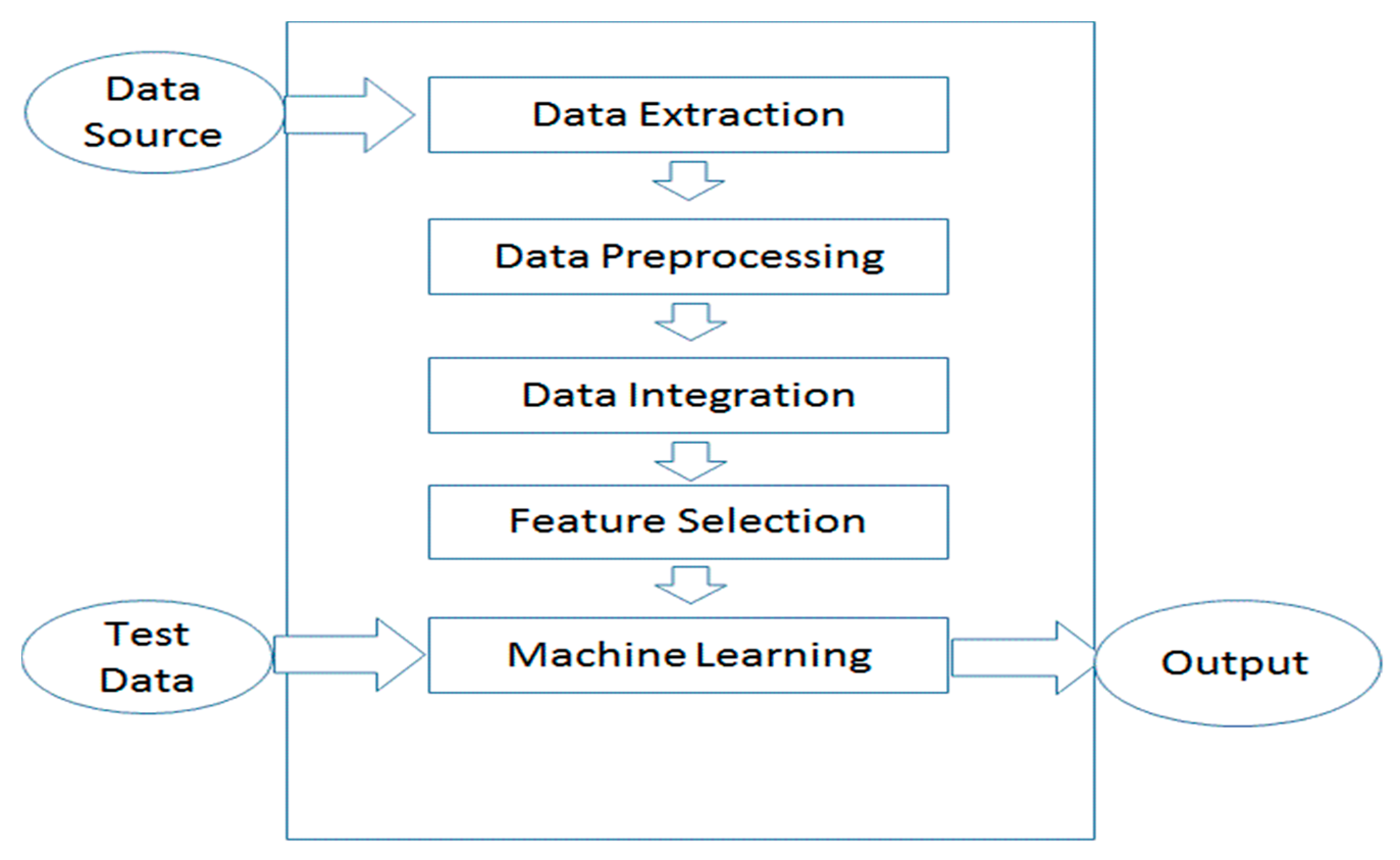
Figure 1 shows the roadmap of data analysis. As depicted in Figure 1, Steps 1 through 4 are data extraction, data preprocessing, data integration, and feature selection. Then, a regression analysis is performed.

Table 1. Summary Statistics during Years 2010–2015.

	# Obs.	Mean	Std. Dev.	25th Perc.	75th Perc.	IQR
Audiences	723	7,606,088	9,950,034	791,486	10,275,941	9,484,454
Box Office	723	61,318,760	80,950,277	6,323,297	82,806,144	76,482,847
Budget	723	47,548,911	51,981,049	11,000,000	64,500,000	53,500,000
Metascore	723	51.61	16.77	39.00	63.00	24.00
Theaters	723	2252.72	1368.85	781.00	3284.50	2503.50

shows the summary statistics of the key variables used in the analysis. There were 719 movies between 2010 and 2015. The mean number of audiences per movie was 7.6 million with a standard deviation of 9.95 million. The IQR was 9.5 million for the audiences. The mean of total revenue of a particular movie (i.e., Box Office) was $61.3 million with a standard deviation of $80.9 million. The mean of total production cost (Budget) was $47.5 million with a standard deviation of $51.9 million. Thus, on average, each movie generated an operating income of $13.6 million. The mean metascore was 51.61 and the mean number of theaters that showed a movie was 2253. Most variables used in the analysis demonstrated highly skewed distributions.

As seen in

Table 2. Rating Information during Years 2010–2015.

Rating	G	PG	PG-13	R	NC-17
Frequency	9	101	282	330	1
Proportion	0.0124	0.1397	0.39	0.4564	0.0014

Note: G = General Audiences, PG = Parental Guidance Suggested, PG-13 = Parents Strongly Cautioned, R = Restricted (under 17 requires accompanying parent or adult guardian), and NC-17 = Adults Only.

, the “R” rating is the most frequent (n = 330) rating for movies, followed by “PG-13” (n = 280) between 2010 and 2015. These two ratings accounted for about 85 percent of all ratings. There are very few movies with “NC-17” or “G”.

Since the data size has become larger, complicated, and highly correlated among many variables, machine learning research has been very popular over the last two decades because machine learning techniques can be applied to big, complicated, and highly correlated data, which has been a difficult issue to be dealt with using generalized linear regression methods. Recently, many different variants of machine learning techniques have been applied to the economic success of the movie industry, but machine learning research on the economic success of the movie industry were mostly focused on classification methods. So, we want to propose machine learning regression methods for modeling the financial success of movies. This is the strong research motivation in this paper.

With the movie data described in this session, we define the financial success of the movie industry as ROI (return on investment) with box office and budget variables as follows:

$$ROI=\frac{Boxoffice-Budget}{Budget}\times 100\%$$

In terms of the film industry’s marketing viewpoint, we focus on modeling ROI with important variables selected by the Bayesian variable selection method. The higher the ROI is, the more profitable a movie is, and vice versa.

Table 3. Summary Statistics for ROI during Years 2010–2015. Unit is Percent (%).

ROI	Statistics
Sample Size (n)	719
Mean	755.8263
Std. Dev.	1559.7506
Variance	2,432,822.029
Range	1559.7506
25th percentile	−65.5669
75th percentile	105.1934
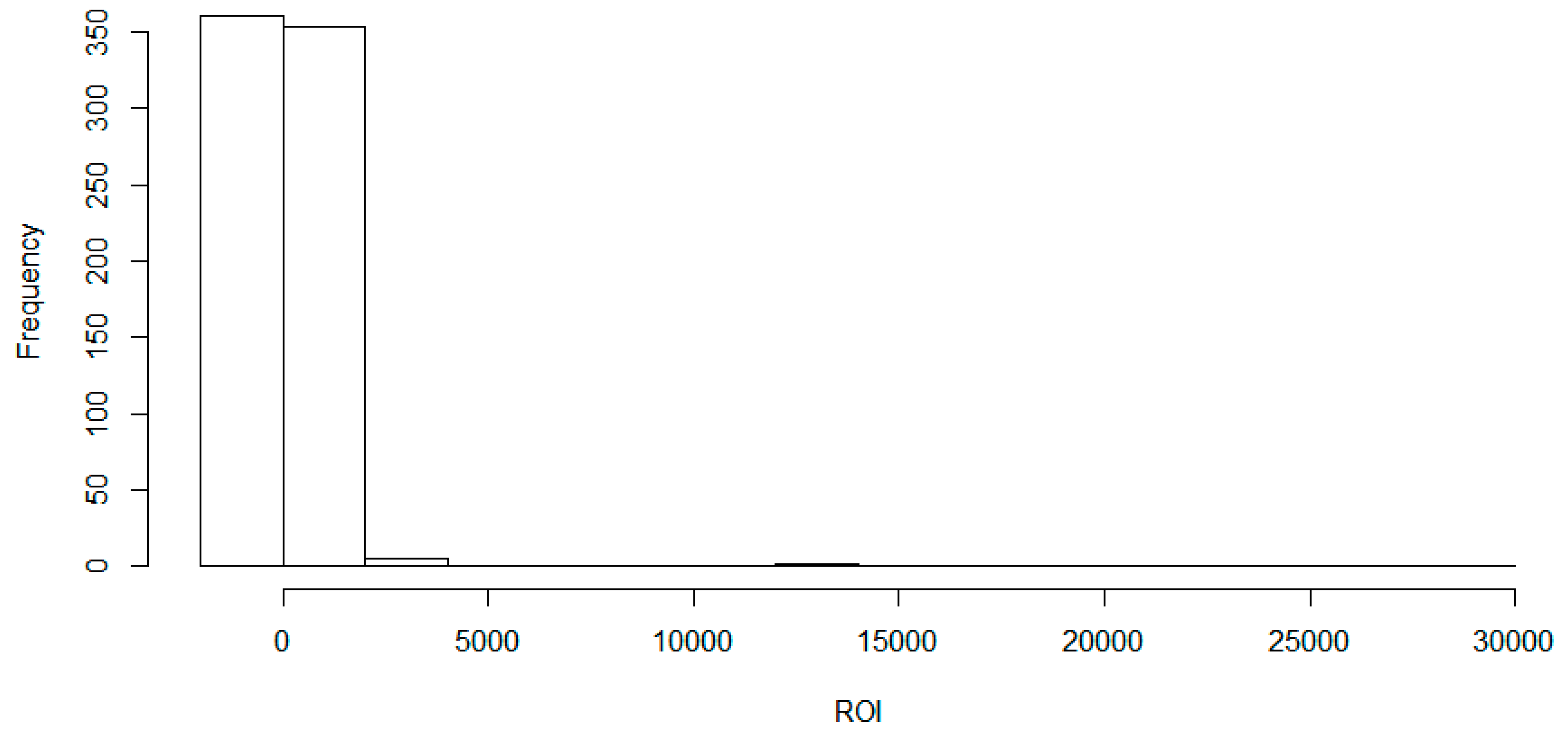
IQR	170.7602

shows that the bottom 25 percent of ROI has a negative number. In Figure 2, the earning rate is skewed to the right. This means that most movies earn in the low range of the ROI, with a few exceptions that are distributed on a large range (long “tail”) of the higher ROI.

3. Bayesian Variable Selection and Machine Learning Methods

We use the Bayesian variable selection and statistical machine learning methods in this research. We apply the Bayesian variable selection method to Hollywood movie data. In this Section, we briefly explain the Bayesian variable selection. Objective Bayesian methods for hypothesis testing and variable selection in linear models are considered in Garcia-Donato and Forte (2018). Garcia-Donato and Forte (2018) introduce the usage of specific functions to compute several types of model averaging estimations and predictions weighted by posterior probabilities. BayesVarSel contains exact algorithms to perform fast computations in problems of small to moderate size and heuristic sampling methods to solve large problems. So, we applied GibbsBvs function with gZellner prior, the number of iterations = 10,000 and the number of burninng = 1000 in ‘BayesVarSel’ R package [Garcia-Donato and Forte (2018)] to the described variables in the Section 2.

Quantile regression is an extension of the classical regression that offers information on the whole conditional distribution of the response variable. If in the classical regression case the goal is to approximate the conditional mean, in quantile regression the focus is to approximate the conditional quantile functions of a response variable Y given a set of variables X. The quantile regression model can capture the information associated with the location, scale and the shape shift of the conditional distribution, it is useful when heteroskedasticity is involved and in homogeneous regression models where the usual parametric assumptions do not hold. No error distribution is imposed in quantile regression. Quantile regression estimators have the equivariance property as the ordinary least square estimators but the equivariance to monotone transformations is specific only to quantile regression. Davino et al. (2014) provide excellent sources for various properties of quantile regression as well as many computer algorithms.

Friedman (1991) introduced multivariate adaptive regression splines (MARS) which is a non-parametric regression technique that automatically simulates nonlinearities and interactions between variables. MARS builds models of the form

$$\widehat{f}\left(x\right)={\displaystyle \sum }_{i=1}^n{C}_i{B}_i\left(x\right)$$

where the model is a weighted sum of the base functions $B_i$ and $C_i$, which are constant coefficients. To apply MARS to Hollywood movie data, we used earth function with default in ‘earth’ R package.

Smola and Schölkopf (2004) described that the SVM algorithm is a nonlinear generalization of the Generalized Portrait algorithm in (Vapnik and Lerner 1963; Vapnik and Lerner 1963; Hastie et al. 2009). In terms of this industrial film context, SVM research has been a good modeling direction for predicting the economic success of a film. In machine learning, SVMs are supervised learning models related to learning algorithms that analyze data used for classification and regression analysis. To apply SVM Regression to Hollywood movie data, we used ksvm function with default in ‘kernlab’ R package. We used the radial basis function kernel, or RBF kernel, which is a popular kernel function used in various kernelized learning algorithms, especially in support vector machine classification.

We also set cost parameter to be 5. While the greater cost parameter penalizes large residuals, the resultantly decreased bias offers a more flexible model with fewer misclassifications. The cross-validation error is 3.

Kaur and Nidhi (2013) built a mathematical model for predicting the success class, i.e., flop, hit, super hit, of Indian movies. In order to accomplish this, Kaur and Nidhi (2013) developed a methodology in which the historical data of each part (e.g., actor, actress, director, music) that affects the success or failure of a movie is given in weight and age and then based on multiple thresholds computed on the basis of descriptive statistics of the dataset of each component. It is then given a class (flop, hit, super hit) label. Then the dataset is subjected to a neural network-based learning algorithm for automating the process. The results in terms of a match between actual class labels and predicted labels are evaluated. The results indicate that the strategy of recognizing the class of success is extremely effective and accurate, which is obvious from the classification matrix. In machine learning or cognitive science, an artificial neural network (ANN) is a network inspired by biological neural networks which are used to estimate functions that can rely on a great number of inputs that are unknown. To apply single-hidden-layer neural network to Hollywood movie data, we used nnet function with single layer with five neurons in ‘nnet’ R package. We set the size number of neurons in the hidden layer to be 20 for 2010–2015 years data and to be 10 with 2010–2014 in this paper. We set the decay parameter for weight decay to be 1 and switch for linear output units.

4. Empirical Results

In this section, we want to compare the traditional linear regression requiring several assumptions that we previously mentioned and the popular machine learning methods for modeling ROI by in-sample forecasting and out of sample forecasting.

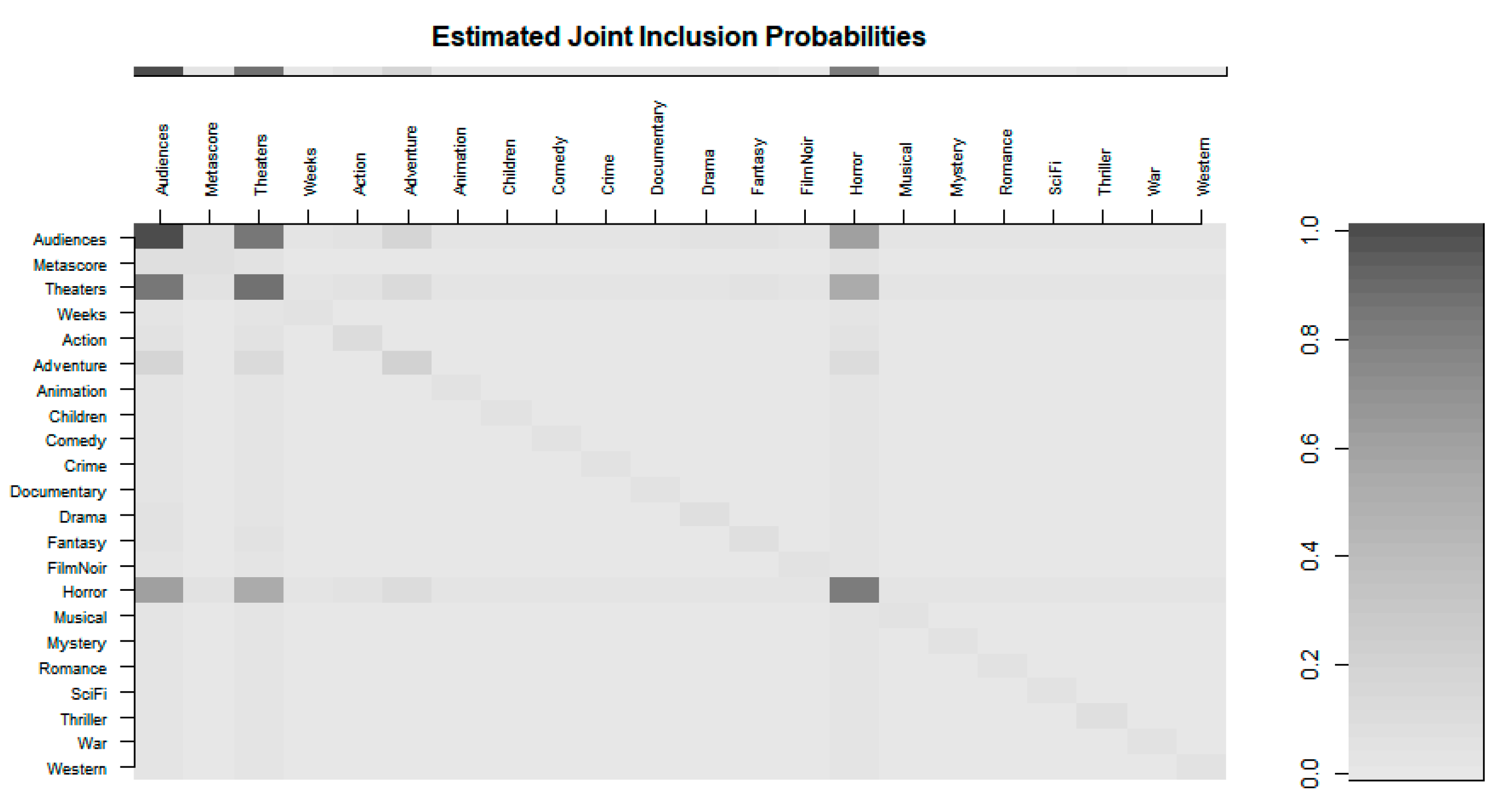
We select the most important predictive variables that determine ROI by using one of the most popular machine learning methods, the Bayesian variable selection method. Figure 3 and

Table 4. Bayesian variable selection method for ROI during Years 2010–2015.

Variable	Inclusion Probability	HPM	MPM
Audiences	0.6733	*	*
Metascore	0.0646
Theaters	0.5878	*	*
Weeks	0.0451
Action	0.0752
Adventure	0.1473
Animation	0.0471
Children	0.0421
Comedy	0.0356
Crime	0.0347
Documentary	0.0398
Drama	0.0521
Fantasy	0.0647
FilmNoir	0.0386
Horror	0.5474	*	*
Musical	0.0381
Mystery	0.0454
Romance	0.0421
SciFi	0.0370
Thriller	0.0514
War	0.0407
Western	0.0394

Note: HPM stands for Highest posterior Probability Model and MPM for Median Probability Model. * means statistically significant at the 5% significance level.

display the importance level of predictors for ROI during years 2010–2015. More useful variables achieve higher accuracy.

Based on the Bayesian variable selection method, we selected the following three important variables as audiences, theaters and horror for the explanatory variable to output variable ROI modeling during years 2010–2015.

The histogram of ROI during Years 2010–2015 in Figure 2 show that there is an extremely skewed distribution. There are many films with a low ROI, and some are highly successful. The traditional regression analysis is not appropriate with this Hollywood data so that we used quantile regression (QR) such as 25th quantile regression (QR25), 50th quantile regression (QR50) and 75th quantile regression (QR75).

In

Table 5. Quantile Regression of ROI with 2010–2015 Years data.

25th Percentile Regression	Estimate	Standard Error	t-Value
(Intercept)	−98.69501	5.56383	−17.73869
Audiences	0.00000	0.00000	6.43183
Theaters	0.01209	0.00293	4.12331
Horror	0.76201	14.30223	0.05328
Median Regression	Estimate	Standard Error	t-Value
(Intercept)	−83.03021	6.62744	−12.52824
Audiences	0.00000	0.00000	6.79277
Theaters	0.01699	0.00357	4.76616
Horror	16.51633	17.49050	0.94430
75th Percentile Regression	Estimate	Standard Error	t-Value
(Intercept)	−1.06583	16.67615	−0.06391
Audiences	0.00001	0.00000	3.72178
Theaters	0.00508	0.01016	0.49990
Horror	363.79949	109.55334	3.32075

, the outputs of quantile regression clearly show that ROI will be statistically increased as the more theaters increasing because the formula of ROI is based on two variables (Budget and Box Office). The interesting findings from QR50 and QR75 in Table 5 are that ROI will be statistically significantly increased with the increase of the horror genre and that intercept is statistically positive significant to ROI, which means the average of ROI during years 2010–2015 increased.

From

Table 6. RMSE of ROI with 2010–2015 Years data (in-sample forecast).

Models	QR25	QR50	QR75	MARS	SVM	NNet
RMSE	1581.893	1576.173	1555.238	1420.817	1308.136	1179.089

, Neural network (NNet) model has the smallest RMSE (root-mean-square error) value for ROI for Year with 2010–2015 Years data (in-sample forecasting) compared with the values of RMSEs of QR25, QR50, QR75, MARS and SVM. In terms of in-sample forecasting, the machine learning methods such as MARS, SVM and NNet are superior than quantile regression. Especially, NNet is the best among MARS, SVM, and NNet with this Hollywood data.

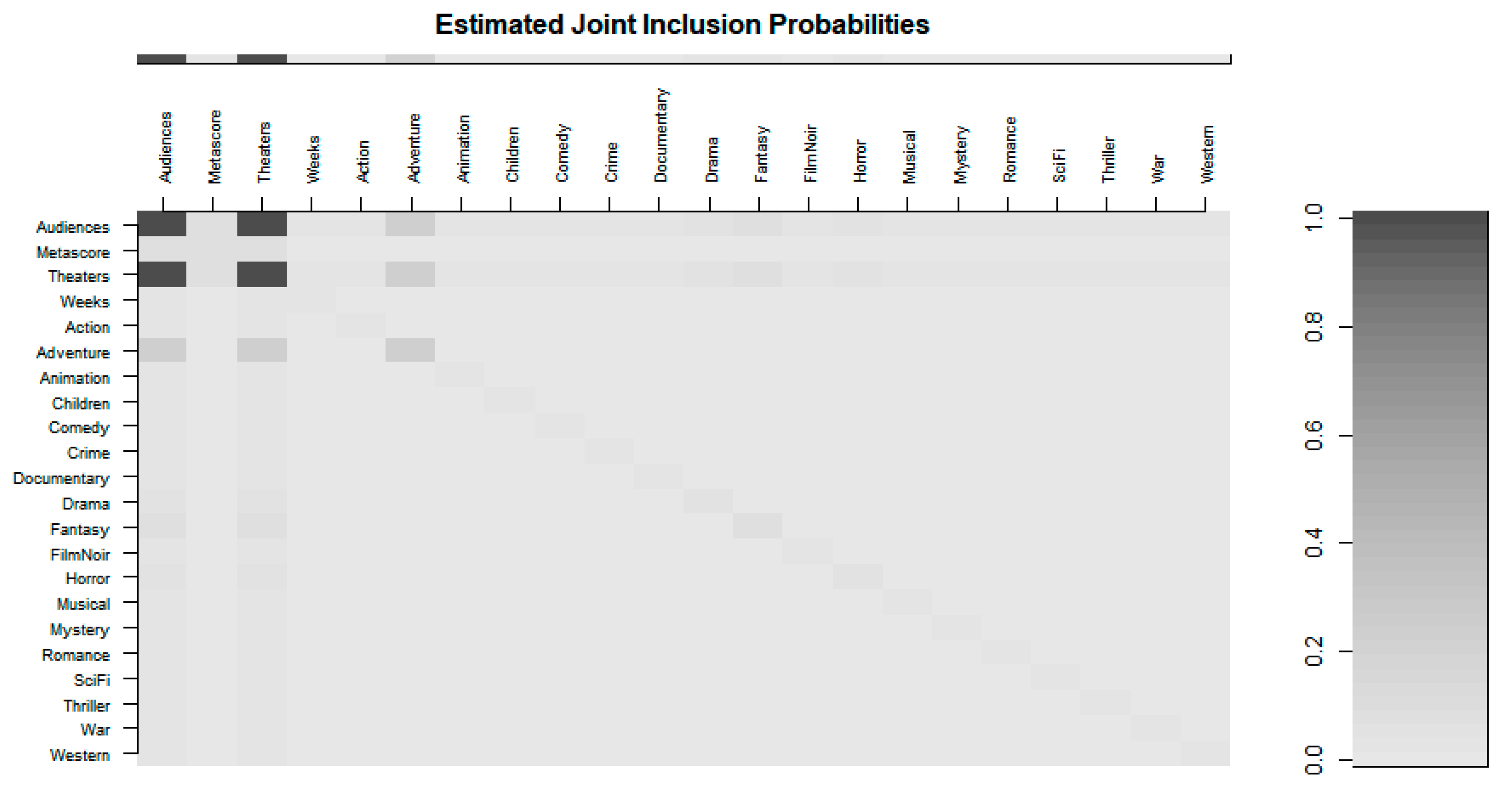
By the Bayesian variable selection method, we also selected the most important predictive variables that determine ROI,

Table 7. Bayesian variable selection of ROI with Movie Data (2010–2014).

Variable	InclusionProbability	HPM	MPM
Audiences	0.9985	*	*
Metascore	0.0816
Theaters	0.9970	*	*
Weeks	0.0400
Action	0.0424
Adventure	0.2340
Animation	0.0491
Children	0.0413
Comedy	0.0496
Crime	0.0450
Documentary	0.0429
Drama	0.0611
Fantasy	0.0802
FilmNoir	0.0346
Horror	0.0612
Musical	0.0428
Mystery	0.0506
Romance	0.0471
SciFi	0.0414
Thriller	0.0386
War	0.0498
Western	0.0400

Note: HPM stands for Highest posterior Probability Model and MPM for Median Probability Model. * means statistically significant at the 5% significance level.

and Figure 4 display the Audiences and Theaters variables for the explanatory variable to output variable ROI modeling during years 2010–2014.

In

Table 8. Quantile Regression of ROI with 2010–2014 Years data.

25th Percentile Regression	Estimate	Standard Error	t-Value
(Intercept)	−98.59969	5.38054	−18.34761
Audiences	0.00000	0.00000	5.73186
Theaters	0.01221	0.00301	4.06243
Median Regression	Estimate	Standard Error	t-Value
(Intercept)	−79.05235	6.38368	−12.55561
Audiences	0.00000	0.00000	7.12540
Theaters	0.01571	0.00353	4.54326
75th Percentile Regression	Estimate	Standard Error	t-Value
(Intercept)	17.87768	21.16789	0.51878
Audiences	0.00001	0.00000	3.98656
Theaters	−0.00484	0.01133	0.04941

, the outputs of quantile regression clearly show that ROI will be statistically increased as the more theaters increasing. However, the interesting finding from QR25 and QR50 in Table 8 are that Intercept is negatively statistical significant to ROI. This means the average of ROI during years 2010–2014 was decreased.

We also divided two data sets which are train data (years 2010–2014) and test data (year 2015) to compare the forecasting prediction accuracy with QR25, QR50, QR75, MARS, SVM, and neural network models. For a measure of prediction accuracy of a forecasting method, we employed the mean absolute percentage error (MAPE) used as a loss function for regression problems in machine learning. The formula of MAPE is defined as

$$MAPE=\frac{1}{n}{\displaystyle \sum }_{i=1}^n\left|\frac{O_i-P_i}{O_i}\right|$$

where $O_i$ is the actual value and $P_i$ is the forecast value. The absolute value in this formula is summed for every forecasted point in time and divided by the number of fitted points n.

In

Table 9. MAPE of ROI for Year 2015 with 2010–2014 Years data (out of sample forecast).

Models	QR25	QR50	QR75	MARS	SVM	NNet
MAPE	2.866375	1.792536	6.611668	12.22441	3.507784	5.298819

, among those six models above, we can clearly see that QR50 model has the smallest MAPE compared with the other five models (QR25, QR75, MARS and SVM and NNet) in terms of ROI. 7. To perform the graphical comparison of forecasts by each model, we used boxplots of the absolute percentage errors for each model in Figure 5.

Table 10. Summary Statistics of Absolute Percentage Errors of ROI for Each Model for Year 2015 with 2010–2014 Years data (out of sample forecast).

Model	QR25	QR50	QR75	MARS	SVM	NNet
Minimum	0.0130	0.0588	0.0591	0.0704	0.0866	0.0559
1st Quantile	0.4408	0.5330	0.7210	0.9912	0.5008	0.5131
Median	1.0080	0.8826	1.2839	2.1983	0.9808	1.1768
Mean	1.9197	1.5228	4.5124	7.0172	3.5078	5.2988
3rd Quantile	1.2994	1.1014	3.7177	4.9271	2.0645	2.5618
Maximum	39.754	24.175	88.996	102.031	57.461	121.833
IQR	0.8586	0.5685	2.9967	3.9359	1.5638	2.0487

shows that QR50 model has the smallest median and interquartile range (IQR) among the seven forecasting models. The results in Table 10 conformed to Figure 5.

To do the statistical tests to show the differences between models for MAPEs of ROI, we use Wilcoxon rank sum test and median test. For the Wilcoxon rank sum test, we rank all N observations. The sum W of the ranks for the first sample is the Wilcoxon rank sum statistic. If the two populations have the same continuous distribution, then W has mean

$${\mu }_W=\frac{n_1\left(N+1\right)}{2}$$

and its standard deviation is

$${\sigma }_W=\sqrt{\frac{n_1{n}_2\left(N+1\right)}{12}}.$$

The Wilcoxon rank sum test rejects the hypothesis that the two populations have identical distributions when the rank sum W is far from its mean.

When the distribution may not be normal, we state the hypotheses in terms of population medians rather than means.

$$H_0:media{n}_1=media{n}_2$$

$$H_a:media{n}_1\ne media{n}_2$$

In

Table 11. The statistical tests to show the differences between models for the absolute percentage errors of ROI for each model.

	QR50
Test	Wilcoxon Rank Sum Test (p-Value)	Median Test (p-Value)
QR2	0.4703	0.2772
QR75	0.0032	0.0294
MARS	0.0000004	0.00001
SVM	0.2472	0.7174
NNet	0.0426	0.0294

, we used Wilcoxon rank sum test and median test to show the differences between QR50 and one of other six models with the absolute percentage errors of ROI for each model. Table 11 shows that there are statistically differences between QR 50 and one of the five models (QR75, MARS and NNet), but there is not statistical difference between QR 50 and QR25 or QR 50 and SVM by both Wilcoxon rank sum test and median test.

In Table 9, we showed that QR50 has the smallest MAPE compared with the other five models (QR25, QR75, MARS, SVM and NNet) in terms of ROI. In Table 10, QR50 has the smallest median and IQR of the absolute percentage errors of ROI among six forecasting models. Therefore, in terms of out of sample forecasting for ROI, we can conclude that the QR50 model is superior than the QR25, QR75, MARS, SVM, and NNet models, even though the MAPEs of QR25 and QR50, SVM, and QR50 are not statistically significant at the 5% significance level.

5. Conclusions

We employed modern statistical methods to Hollywood movie data. Rather than using all variables in our data, we used the selective and important predictive variables for ROI by using the Bayesian variable selection method. By performing this approach, we can avoid not only the possible measurement error in the Hollywood dataset, but also the unnecessary statistical conditions such as multicollinearity and independence among the explanatory variables for ROI. Our results showed that the neural network Model for ROI is overall superior to the well-known machine learning methods in terms of RMSE for in-sample forecasting and the median quantile regression model for ROI is overall superior to the well-known machine learning methods in terms of MAPE for out of sample forecasting. For future research, we will apply the quantile regression and machine learning methods to the Hollywood movie keyword count data generated by the text mining technique to obtain the relationship between movie title keywords and ROI.