A Hypothesis Test Method for Detecting Multifractal Scaling, Applied to Bitcoin Prices

Abstract

Multifractal processes reproduce some of the stylised features observed in financial time series, namely heavy tails found in asset returns distributions, and long-memory found in volatility. Multifractal scaling cannot be assumed, it should be established; however, this is not a straightforward task, particularly in the presence of heavy tails. We develop an empirical hypothesis test to identify whether a time series is likely to exhibit multifractal scaling in the presence of heavy tails. The test is constructed by comparing estimated scaling functions of financial time series to simulated scaling functions of both an iid Student t-distributed process and a Brownian Motion in Multifractal Time (BMMT), a multifractal processes constructed in Mandelbrot et al. (1997). Concavity measures of the respective scaling functions are estimated, and it is observed that the concavity measures form different distributions which allow us to construct a hypothesis test. We apply this method to test for multifractal scaling across several financial time series including Bitcoin. We observe that multifractal scaling cannot be ruled out for Bitcoin or the Nasdaq Composite Index, both technology driven assets.

1. Introduction

The cryptocurrency market is an emerging market comprised of thousands of digital assets including Bitcoin. A cryptocurrency is a digital asset that uses cryptography and decentralised governance to secure a ledger of transactions. Cryptocurrencies can also be used as a medium of exchange; for background, refer to the review article by Milutinović (2018). Bitcoin, introduced in Nakamoto (2009), is an example of the world’s first cryptocurrency; its core innovation established digital scarcity, regulated and audited via a novel decentralised governance mechanism. Financial analysts, chartists and the news media often report on Bitcoin’s fractal features (Chambers 2019); however, academic research has shown mixed evidence for multifractal or monofractal scaling with Mensi et al. (2019); Lahmiri and Bekiros (2018); Stavroyiannis et al. (2019) presenting a case for multifractal scaling, while Nadarajah and Chu (2017); Bariviera (2017); Bariviera et al. (2017); Zhang et al. (2018) presenting a case for monofractal scaling. The inconclusive evidence of fractal scaling could be a result of the different detection methods along with varied assumptions. Salat et al. (2017) emphasise that implementation of existing multifractal detection methods can be a perilous undertaking. Moreover, Sly (2006) and Grahovac and Leonenko (2014) demonstrate that attempts to use the scaling function to detect multifractality may mistakenly give rise to false positive results, due to heavy-tailed effects. This calls into question the reliability of the above-mentioned results. Therefore, a detailed examination of scaling functions in the presence of heavy tails is required to bridge the gap between the theory and empirical realities. As an application of the new method we present here, we seek to understand Bitcoin’s scaling properties to assist practitioners with model selection for the purpose of risk management and volatility forecasting. Given the novel nature of digital assets, it is also of interest to observe similarities in scaling behaviour between Bitcoin and other asset classes. In this paper, we address the central research question: Do Bitcoin prices exhibit multifractal scaling? To answer this question, we investigate the effect of heavy-tails on the scaling function and study scenarios in which false positive1 detection occurs. If multifractal scaling is plausible, it could indicate the need to incorporate more complex scaling behaviour into pricing models. In the case of Bitcoin, capturing complex scaling behaviour could result in better volatility forecasting. This paper develops an empirical method that tests for multifractal scaling in the presence of heavy tails. Its application is not limited to financial time series, however. This paper is structured as follows. In the rest of this section, we introduce multifractal stochastic processes and their simulation methods. We then explain how the multifractal scaling function is distorted by the presence of heavy tails. In Section 2, we propose a new empirical hypothesis test and construct the look-up table to form rejection and acceptance regions. Then, in Section 3, we apply our hypothesis test to detect multifractal scaling in Bitcoin prices and compare the scaling behaviour of Bitcoin to other financial assets, including the S&P500 index, the Nasdaq Composite Index, the USD/JPY exchange rate, and Gold Futures. Our method detects more complex scaling behaviour in emerging technology asset classes such as Bitcoin and the Nasdaq Composite Index.

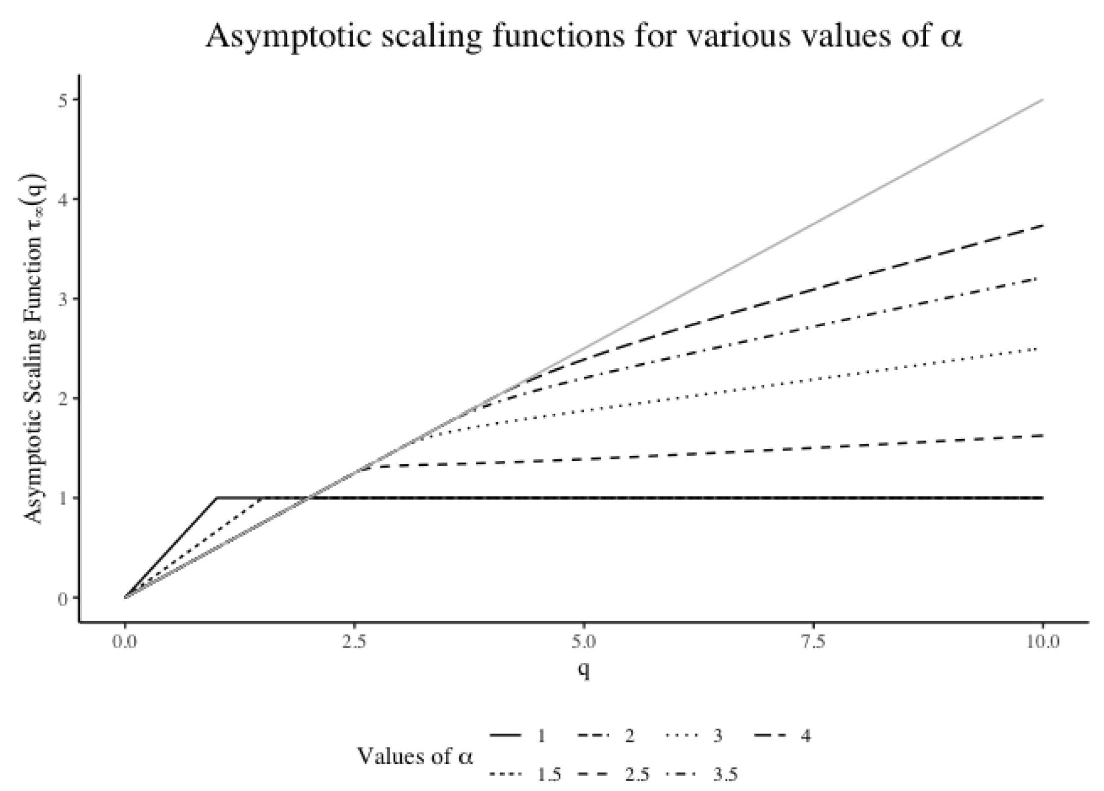
1.1. Monofractal vs. Multifractal Processes

The multifractal system was introduced as a generalisation of the fractal system to describe more complicated dynamics in time series. Multifractals are common in nature and have enjoyed great application in finance and science, e.g., modelling the turbulence in fluid dynamics (Sreenivasan 1991). In the finance field, multifractal processes are able to capture many stylised characteristics of high-volatility financial assets.

Multifractal processes are defined based on the scaling property of their moments, when they are finite, in Mandelbrot et al. (1997).

Definition 1.

(Multifractal Stochastic Process) A stochastic process $\left\{X\right(t),t\ge 0\}$ is multifractal if it has stationary increments and there exist functions $c\left(q\right)>0$ and $\tau \left(q\right)>0$ and positive constants $\mathcal{Q}$ and $\mathcal{T}$ such that

$${\mathbb{E}\left|X\left(t\right)\right|}^q=c\left(q\right)t^{\tau \left(q\right)},\mathit{for}\mathit{all}q\in [0,\mathcal{Q}]\mathit{and}t\in [0,\mathcal{T}].$$

(1)

The function $\tau \left(q\right)$ is called the scaling function.

The multifractal processes are said to be multiscaling when the scaling function is nonlinear. For a multifractal process, the scaling function $\tau \left(q\right)$ is always concave when $q>0$ on a bounded interval as is shown in Sly (2006).

In contrast, the multifractal process is called uniscaling or a monofractal process when the scaling function is linear, $\tau \left(q\right)=Hq$. Monofractal processes enjoy a self-similarity.2

Theorem 1.

(Lamperti (1962)). If $\left\{X\right(t),t\ge 0\}$ is self-similar and stochastically continuous at t = 0, then there exists a unique $H>0$ such that for all $a>0$,

$$\left\{X\left(at\right)\right\}\stackrel{d}{=}\left\{a^{H}X\left(t\right)\right\}$$

(2)

where equality is of finite dimensional distributions.

Here, $H\ge 0$ is a constant known as the Hurst parameter. H measures in some way the persistence of a process. Given all moments of the process are finite, the process is long-range dependent if $H\in (\frac{1}{2},1)$, while anti-persistence occurs if $H\in (0,\frac{1}{2})$ (Embrechts and Maejima 2000). Typical examples of monofractal processes are the fractional Brownian motions and the stable Lévy processes. The fractional Brownian motion $B_H\left(t\right)$ introduced in Mandelbrot et al. (1997) is a unique class of self-similar Gaussian process with stationary increments possessing a dependence structure described by the following covariance equation. When $H=\frac{1}{2}$, the fractional Brownian motion becomes Brownian motion with independent increments.

1.2. Examination of Multifractality

Copious methods have been proposed to examine the multifractality in a certain process $\left\{X\right(t),0\le t\le T\}$, including the multifractal detrended fluctuation analysis method (MF-DFA) by Kantelhardt et al. (2002) and the wavelet transform modulus maxima method (WTMM). In this paper, we employ the standard partition method introduced by Mandelbrot et al. (1997). This method attempts to detect multifractality based on concavity in the scaling function. From Definition 1, one can easily derive

$${log\mathbb{E}\left|X\left(t\right)\right|}^q=logc\left(q\right)+\tau \left(q\right)logt,\mathrm{for}\mathrm{all}q\in [0,\mathcal{Q}]\mathrm{and}t\in [0,T],$$

(3)

where the q-th moment of the process $X\left(t\right)$, ${\mathbb{E}\left|X\left(t\right)\right|}^q$, can be estimated by the sample statistic

$$S_q(T,\Delta t)=\frac{1}{N}\sum _{i=1}^N{|X((i-1)\Delta t)-X(i\Delta t)|}^q,$$

(4)

with $N=\lfloor T/\Delta t\rfloor$.

The scaling function can be derived by fitting a linear regression between $log{S}_q(T,\Delta t)$ and $logt$ with various values of $q\in [0,\mathcal{Q}]$. For a fixed value of q, we obtain an estimate $\widehat{\tau }\left(q\right)$, the slope of our linear regression. A plot of $\widehat{\tau }\left(q\right)$ against q then provides visual display of the scaling function. The function of $ln{S}_q(T,\Delta t)$ for various values of $ln\Delta t$ is called the partition function. If the scaling function shows concavity, we have evidence that multifractality is present in the process of interest.

1.3. Simulation of Multifractal Processes

The Brownian motion in multifractal time (BMMT) $B_H\left(\theta \left(t\right)\right)$ introduced in Mandelbrot et al. (1997) is employed to simulate a multifractal process. The BMMT model shows appealing features that coincide with some stylised features of financial time series. It displays heavy-tails while not necessarily implying infinite variance. It also implies long-term dependence in absolute values of returns while the price increments themselves can remain uncorrelated. By construction, the BMMT is defined as the subordinate model of a fractional Brownian motion $B_H\left(t\right)$ with a multifractal process $\theta \left(t\right)$.

Definition 2.

(Brownian Motion in Multifractal Time). Brownian motion in multifractal time is defined as

$$X\left(t\right)=B_H\left(\theta \left(t\right)\right),t\in [0,T],$$

where $\theta \left(t\right)$ is a positive multifractal stochastic process and $B_H$ is an independent fractional Brownian motion with Hurst parameter H.

$\theta \left(t\right)$ can also be seen as a trading time where the index t denotes clock time. We assume the activity time $\theta \left(t\right)$ to be the cumulative density function of a random multifractal measure $\mu$ defined on $[0,T]$. That is, $\theta \left(t\right)$ is a multifractal process with continuous, non-decreasing paths, and stationary increments.

The multiplicative multifractal measure is implemented for simulation. Without loss of generality, we assume that the time series of interest is defined on a compact interval $[0,1]$. A multiplicative measure is constructed as follows:

• In Stage 1, divide the time interval $[0,1]$ into $b>1$ non-overlapping subintervals with equal length $1/b$. Assign multipliers $M_{1,\beta }(0\le \beta \le b-1)$ to each subinterval, where the $M_{1,\beta }$ are random variables with distributions that are not necessarily discrete. For computational convenience, we assume the $M_{1,\beta }$ to be identically distributed with a common distribution M.
• In Stage 2, each of the b intervals is further divided into b subintervals of length $1/b^2$. Again, we assign multipliers $M_{2,\beta }(0\le \beta \le b-1)$ to each subinterval. The $M_{2,\beta }$ are assumed to be identically distributed with distribution M. Thus, after the second stage, the mass on an interval, for example $[0,1/b^2]$, will be ${\mu }_2[0,1/b^2]=m_0{m}_1$ if $M_{1,0}=m_0$ and $M_{2,0}=m_1$ with probability

  $$\mathbb{P}({\mu }_2[0,1/b^2]=m_0{m}_1)=\mathbb{P}(M=m_0)P(M=m_1),$$

  since the multipliers at different stages are independent. The measure ${\mu }_2$ represents the multiplicative measure at Stage 2.
• Repetition of this scheme generates a sequence of measures ${\left({\mu }_k\right)}_{k\in \mathbb{N}}$ which converges to our desired multiplicative measure $\mu$ as $k\to \infty$.

Remark 1.

To preserve the mass at each stage, some restrictions are required on the values of the $M_{l,\beta },1\le l\le k$. If we strictly assume that ${\sum }_{\beta =0}^{b-1}{M}_{l,\beta }=1$ at each stage, the resulting measure is called microcanonical or micro-conservative. If we loosen the assumption so that the mass at each stage is only conserved “on average", that is, $\mathbb{E}\left({\sum }_{\beta =0}^{b-1}{M}_{l,\beta }\right)=1,\forall 1\le l\le k$, the resulting measure is called canonical.

In this paper, we only consider canonical measures, as they impose less restriction on the distribution of M. Let

$$t=0.{\eta }_1\dots {\eta }_k=\sum _{i=1}^k{\eta }_i{b}^{-i}$$

be a b-adic number and set $\Delta t=b^{-k}$. The mass on the b-adic cell $[t,t+\Delta t]$ for a canonical measure at Stage k is

$$\mu (\Delta t)=\mu [t,t+\Delta t]=\Omega ({\eta }_1,\dots ,{\eta }_k)M\left({\eta }_1\right)M({\eta }_1,{\eta }_2)\dots M({\eta }_1,\dots ,{\eta }_k),$$

where the random variable $\Omega$ represents the total mass. The high-frequency component $\Omega ({\eta }_1,\dots ,{\eta }_k)$ is assumed to have the same distribution as $\Omega$. It captures changes in total mass of the interval caused by stages beyond k. As $\mu$ here is a canonical measure, we assume the multipliers $M_{l,\beta }$ $(0\le \beta \le b-1)$ satisfy $\mathbb{E}(\sum M_{l,\beta })=1$ or equivalently $\mathbb{E}M=1/b.$

Since multipliers at different stages of subdivision are independent, $\mathbb{E}\left[\mu {(\Delta t)}^q\right]=\mathbb{E}\left({\Omega }^q\right){\left[\mathbb{E}\left(M^q\right)\right]}^k,\mathrm{for}\mathrm{all}q.$ Defining $\tau \left(q\right)=-{log}_b\mathbb{E}\left(M^q\right)$ and recalling $\Delta t=b^{-k}$, we have

$$\mathbb{E}\left[\mu {(\Delta t)}^q\right]=\mathbb{E}\left({\Omega }^q\right){(\Delta t)}^{\tau \left(q\right)}.$$

(5)

Consequently, the constructed multiplicative measure $\mu$ is multifractal according to Definition 1. Because Equation (5) only holds for $\Delta t=b^{-k}$ and $t=0.{\eta }_1\dots {\eta }_k={\sum }_{i=1}^k{\eta }_i{b}^{-i}$ being a b-adic number, these multiplicative measures are said to be grid-bound multifractal measures.

The relation between the distribution of M and the scaling function can be inferred from the following theorem.

Theorem 2.

(Calvet et al. 1997). Define $p\left(\alpha \right)$ to be the continuous density of $V=-{log}_{b}M$, and $p_k\left(\alpha \right)$ to be the density of the k-th convolution product of p. The scaling function of a multiplicative measure satisfies

$$\tau \left(q\right)=\underset{\alpha }{inf}[\alpha q-\underset{k\to \infty }{lim}\frac{1}{k}{log}_b\left[k{p}_k\left(k\alpha \right)\right].$$

(6)

In this paper, we have estimated sample scaling functions using the BMMT with a log-normal multiplicative measure. We have chosen this measure because its multifractal spectrum is a better fit for financial time series3. When V follows a normal distribution, $\mathcal{N}(\lambda ,{\sigma }^2)$ where $\lambda >1$, then $M=b^{-V}$ follows a log-normal distribution that is, ${log}_{b}M\stackrel{d}{=}\mathcal{N}(-\lambda ,{\sigma }^2)$. We then have

$$\mathbb{E}M=\mathbb{E}\left(e^{-Vlogb}\right)=exp\left(-\lambda logb+\frac{{(logb)}^2{\sigma }^2}{2}\right),$$

As $M\in (0,\infty )$, we need the constraint $\mathbb{E}\left(M\right)=1/b$ to make M a canonical measure. This constraint gives a relationship between $\lambda$ and ${\sigma }^2$, namely $logb=\frac{2(\lambda -1)}{{\sigma }^2}$.

Based on Theorem 2, the scaling function for the log-normal multiplicative cascade is derived as follows:

$$\tau \left(q\right)=\underset{\alpha }{inf}\left(\alpha q-\underset{k\to \infty }{lim}\frac{1}{k}{log}_b\left[k{p}_{\alpha }\left(k\alpha \right)\right]\right)=\lambda q-\frac{{\sigma }^{2}logb}{2}{q}^2.$$

(7)

This quadratic form reaches its maximum at $q=\frac{\lambda }{{\sigma }^{2}logb}$.

The cumulative distribution of the simulated multiplicative measures $\mu$ gives a multifractal multiplicative cascade, which is taken to be the trading time $\theta \left(t\right)={\int }_0^t\mu \left([0,s]\right)ds$ in a BMMT model $B_H\left(\theta \left(t\right)\right)$.

1.4. Multifractality and Heavy Tails

While a concave scaling function is necessary for multifractality, it is not sufficient. Several papers have explored other potential drivers of concavity in the scaling function. One is heavy-tailedness (Sly 2006; Heyde 2009 and Grahovac and Leonenko 2014). Sly (2006) has shown that, after removing the extreme values of the S&P500 price process, the scaling function approaches linearity. He proceeded further to study the asymptotic behaviour of the estimated scaling functions and proved the following theorem.

Theorem 3.

(Sly 2006). Let X be a random variable with $\mathbb{E}\left(X\right)=0$ such that the distribution function of $\left|X\right|$ has a regularly varying tail of order $-\alpha$ where $\alpha >2$; that is,

$$P\left(\right|X|>x)=x^{-\alpha }L\left(x\right),$$

where $L\left(x\right)$ is slowly varying. Then, for an i.i.d. sequence with distribution X and $q>\alpha$, for each $s\in (0,1)$, with $S_q$ as defined in Equation (4) and the time increment $\Delta t=n^s$,

$$\frac{ln{S}_q(n,n^s)}{lnn}\stackrel{p}{\to }max\left(s+\frac{q}{\alpha }-1,\frac{sq}{2}\right)$$

(8)

as $n\to \infty$, where $\stackrel{p}{\to }$ stands for convergence in probability.

Grahovac and Leonenko (2014) generalised this result to a type $\mathcal{E}$ set of stochastic processes and extended Sly’s (2006) work by investigating the relationship between the asymptotic behaviour of scaling functions and tail indices.

Definition 3

(Type $\mathcal{E}$ stochastic processes). A stochastic process $\left\{X\right(t),t\ge 0\}$ is said to be of type $\mathcal{E}$ if $Y\left(t\right)=X\left(t\right)-X(t-1)$, $t\in \mathbb{N}$, is a strictly stationary sequence having heavy-tailed marginal distribution with index α, satisfying the strong mixing property with an exponentially decaying rate and such that $\mathbb{E}Y\left(t\right)=0$ when $\alpha >1$.

Theorem 4

(Grahovac and Leonenko 2014). Suppose $\left\{X\right(t),0\le t\le T\}$ is of type $\mathcal{E}$ and suppose $\Delta t_i$ is of the form $T^{\frac{i}{N}}$ for $i=1,\dots ,N$. Then, for every $q>0$ and $s\in (0,1)$

$$\underset{N\to \infty }{lim}\underset{T\to \infty }{\mathrm{plim}}{\widehat{\tau }}_{N,T}\left(q\right)={\tau }_{\infty }\left(q\right),$$

(9)

where $\mathrm{plim}$ stands for limit in probability and

$${\tau }_{\infty }\left(q\right)=\begin{array}{c}\hfill \left\{\begin{array}{cc}\frac{q}{\alpha }\hfill & if0<q\le \alpha and\alpha \le 2\hfill \\ 1\hfill & ifq>\alpha and\alpha \le 2\hfill \\ \frac{q}{2}\hfill & if0<q\le \alpha and\alpha >2\hfill \\ \frac{q}{2}+\frac{2{(\alpha -q)}^2(2\alpha +4q-3\alpha q)}{{\alpha }^3{(q-2)}^2}\hfill & ifq>\alpha and\alpha >2.\hfill \end{array}\right.\end{array}$$

(10)

Besides the heavy-tailed effects, other factors are discussed in a number of papers. Matia et al. (2003) concludes that price fluctuations can contribute to concavity of scaling function. Bouchaud et al. (2000) states that another factor is the long range nature of the volatility correlations. Nevertheless, neither of these scenarios excludes the effect of heavy-tailedness. Therefore, we regard the heavy-tailedness as a main contributor to the possible misdetection of multifractality in this paper.

Figure 1 displays the situation considered in Theorem 4. To illustrate the heavy-tailed effect, the estimated scaling functions for both S&P500 Index and 20 Student $t_4$-distributed processes before and after truncating heavy tails are shown in Figure 2.4

2. Methodology

Our hypothesis test aims to identify multifractal scaling in the presence of heavy tails. It is constructed based on the different distributions of concavity measures for various tail indices:

$$\begin{gathered} H_0:\mathrm{The}\mathrm{process}\mathrm{of}\mathrm{interest}\mathrm{is}\mathrm{not}\mathrm{multifractal}. \\ \mathrm{vs.} \\ {H}_A:\mathrm{The}\mathrm{process}\mathrm{of}\mathrm{interest}\mathrm{is}\mathrm{multifractal}. \end{gathered}$$

In this section, we first introduce the measure of concavity and tail index implemented in this paper. Then, we examine the distributions of concavity measures with regard to various tail indices for different processes. The following four instances are chosen: monofractal process (Brownian motion and fractional Brownian motion); Student t-distributed processes with degrees of freedom between 1 and 20; and a multifractal process simulated using BMMT with a log-Normal multiplicative measure.

2.1. Measure of Concavity

The global and localised simplex statistics proposed in Abrevaya and Jiang (2005) are employed. These loosen the assumption of normality and homoscedasticity of the error disturbances, which is required for most other concavity measures.

Definition 4

(Global Simplex Statistics). Assume that

1. 

there is an iid sample ${\left\{(x_i,{ϵ}_i)\right\}}_{i=1}^n$ drawn from the joint distribution of the random variables $(x,ϵ)$, where ϵ is symmetrically distributed about 0 (conditional on x), so that $\mathbb{E}\left({ϵ}_i\right|x_i)=0,i=1,\dots ,n$;

2. 

the observed sample is ${\left\{(y_i,x_i)\right\}}_{i=1}^n$, where $y_i$ is generated by $y_i=f\left(x_i\right)+{ϵ}_i,i=1,\dots ,n,$ and the functional form of f is left unspecified.

Then, for a sample of size n, the global simplex statistic is defined as

$$U_n={\left(\genfrac{}{}{0pt}{}{n}{3}\right)}^{-1}\sum _{1\le t_1\le t_2\le t_3\le n}\mathit{sign}(a_1{y}_{\left[t_1\right]}+a_2{y}_{\left[t_2\right]}-y_{\left[t_3\right]}),$$

(11)

where $t_1,t_2,t_3\in \{1,\cdots ,n\}$,

$$\mathit{sign}\left(q\right)=\left\{\begin{array}{cc}1\hfill & ifq>0,\hfill \\ -1\hfill & ifq<0,\hfill \\ 0\hfill & ifq=0.\hfill \end{array}\right.$$

(12)

and $a_1,a_2$ are non-negative numbers with $a_1+a_2=1$.

Abrevaya and Jiang (2005) proves the asymptotic normality for the global simplex statistic. An interval is considered to be a concave interval if its standardised global simplex statistics $\widetilde{U_n}$ is less than $Z_{\alpha /2}$, where $Z_{\alpha /2}$ is the $(\alpha /2)$-th percentile of the standard normal distribution, vice versa for a convex interval.

For the localised simplex statistic, calculation starts with dividing the time interval $[0,T]$ into $G=\lfloor T/2h\rfloor$ subintervals, where $2h$ is the window width. Let $x_1^{\ast },x_2^{\ast },\dots ,x_G^{\ast }$ denote evaluation points. In this case, they are assumed to be the mid-points of each sub-interval. Then, the sub-population for which the x values fall in a local window is defined to be

$$V_h\left(x^{\ast }\right)=\{(y,x):x^{\ast }-h<x<x^{\ast }+h\}.$$

Definition 5.

Let $p_h\left(x^{\ast }\right)$ be the number of observations in the set $V_h\left(x^{\ast }\right)$. The localised simplex statistic at a given $x^{\ast }$ is then defined as

$$U_{n,h}\left(x^{\ast }\right)={\left(\genfrac{}{}{0pt}{}{p_h\left(x^{\ast }\right)}{3}\right)}^{-1}\sum _{t_1<t_2<t_3}\left(\mathit{sign}(a_1{y}_{\left[t_1\right]}+a_2{y}_{\left[t_2\right]}-y_{\left[t_3\right]})\times \prod _{k=1}^3{K}_h(x_{t_k}-x^{\ast })\right),$$

(13)

where $a_1+a_2=1$ and $K_h\left(v\right)=K(v/h)$ where the kernel function K is to be specified.

In this paper, we assume a uniform kernel function since no addition information is given. Asymptotic normality also holds for the localised simplex statistics. A sub-interval is defined to be concave if $U_{n,h}<Z_{\alpha /2}$, vice versa for the convex case. We define a concavity measure (localised) as the difference in the proportions of the concave intervals and the convex intervals:

$$L_{n,h}=\mathrm{proportion}\mathrm{of}\mathrm{convex}\mathrm{intervals}-\mathrm{proportion}\mathrm{of}\mathrm{concave}\mathrm{intervals}.$$

Here, $L_{n,h}\in [-1,1]$ measures the level of concavity (convexity). Convexity is concluded for the overall interval when $L_{n,h}\in [0,1]$, while we report strict concavity when $L_{n,h}\in [-1,0)$.

As a measure of tail index, the classic Hill’s estimator is implemented. If $X_1,X_2,\dots ,X_n$ is a sequence of independent and identically distributed random variables with distribution function F and n is the sample size, let $X_{(i,n)}$ be the i-th order statistic of $X_1,X_2,\dots ,X_n$. The Hill’s estimator is

$$h_{\left(k\right(n),n)}^{\mathrm{Hill}}={\left(\frac{1}{k\left(n\right)}\sum _{i=n-k\left(n\right)+1}^{n}log\left(X_{(i,n)}\right)-log\left(X_{(n-k(n)+1,n)}\right)\right)}^{-1},$$

(14)

where $k\left(n\right)\in \{1,2,\dots ,n-1\}$ is a sequence to be specified. Under these assumptions, $h_{\left(k\right(n),n)}^{\mathrm{Hill}}$ converges in probability to the true tail index, and is asymptotically normal when $k\left(n\right)\to \infty$.

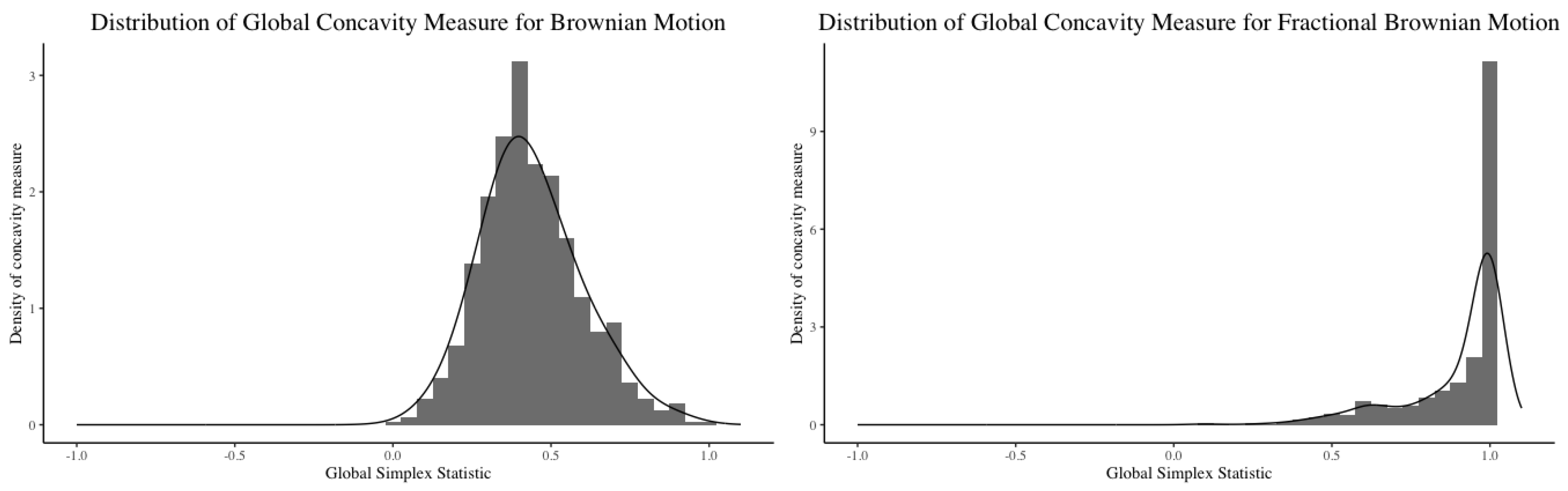
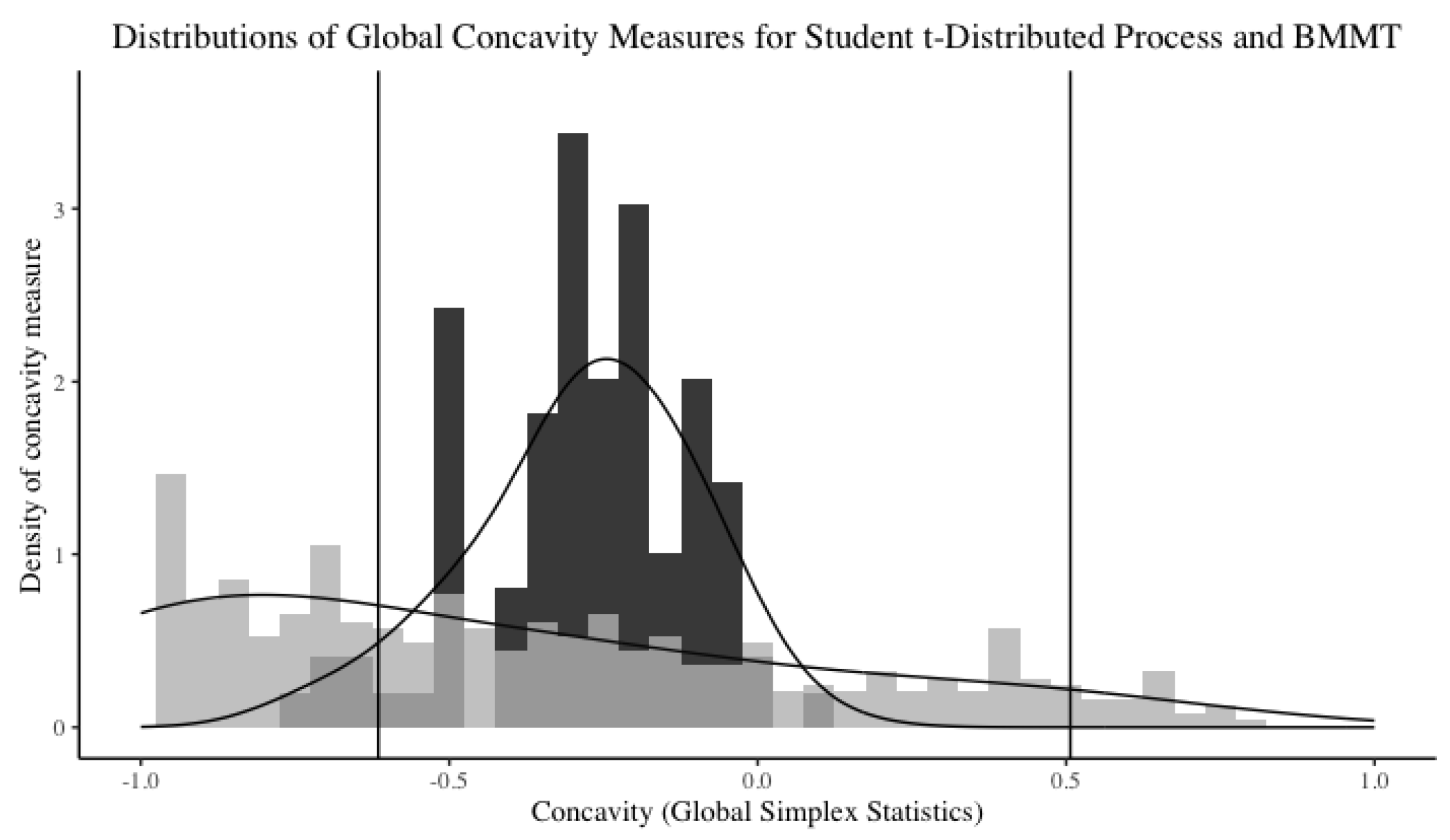
2.2. Simulation Results

We explore the possible range of behaviours for scaling functions for simulated multifractal processes. The findings are compared with some simulated monofractal processes (e.g., Brownian motions and fractional Brownian motions) and Student t-distributed processes. Both Brownian motion and fractional Brownian motion yield convex scaling functions only, which puts them out of consideration in the case of multifractality detection. The distributions of the concavity measures of the simulated multifractal processes and Student t-distributed processes are found to differ significantly in terms of their ranges and skewness. This provides us with a way to design a hypothesis test. As a result of these simulations, we construct a look-up table for a multifractality hypothesis test.

The simulated distributions of both the global and localised5 simplex statistics are quite similar. Here, we only present the simulation results based on the global simplex statistics. The simulation results are shown in Figure 3 and Figure 4. The distributions for the Student t-distributed process and a simulated multifractal process both span $[-1,1]$ but display different characteristics. A detailed comparison for the specific tail index $=3.06$ is shown in Figure 4. For the simulated BMMTs, more than 20% of the scaling functions have global simplex statistics of exactly $-1$ indicating strict concavity. For the Student t-distributed process, the concavity statistic spans $[-1,1]$ with its median at around $-0.36$ in comparison to the one for the simulated BMMTs, $-0.45$.

If the concavity of the observed scaling function for a given process is more severe than for the Student t-distributed processes, we are led to conclude that the concavity is driven by multifractality instead of heavy tails. Therefore, hypothesis tests can be constructed using the concavity measures as the test statistic.

2.3. Look-Up Table

To perform this hypothesis test on a given set of data, we firstly estimate the heaviness of tail using Hill’s estimator $h^{\mathrm{Hill}}$. Then, the null distribution of concavity measures is constructed by simulating from Student t-distributed processes corresponding to tail indices ranging over the interval $[h^{\mathrm{Hill}}-0.5,h^{\mathrm{Hill}}+0.5]$. A larger range of tail index is used to allow for variation in our tail index estimation, while allowing more observations for constructing the concavity measure distribution.6 The 5th percentile of this distribution is the critical value for the hypothesis test.

The null hypothesis is rejected if the observed test statistic is less than the calculated critical value. To carry out the hypothesis test, a look-up table is generated to summarise the tail indices and the corresponding critical values based on both the localised and global concavity measures. A simplified version of the look-up table is presented in Appendix A. The critical values are presented for tail indices 0.5, 1.0, 1.5, …, with the largest tail index being 10.

3. Results

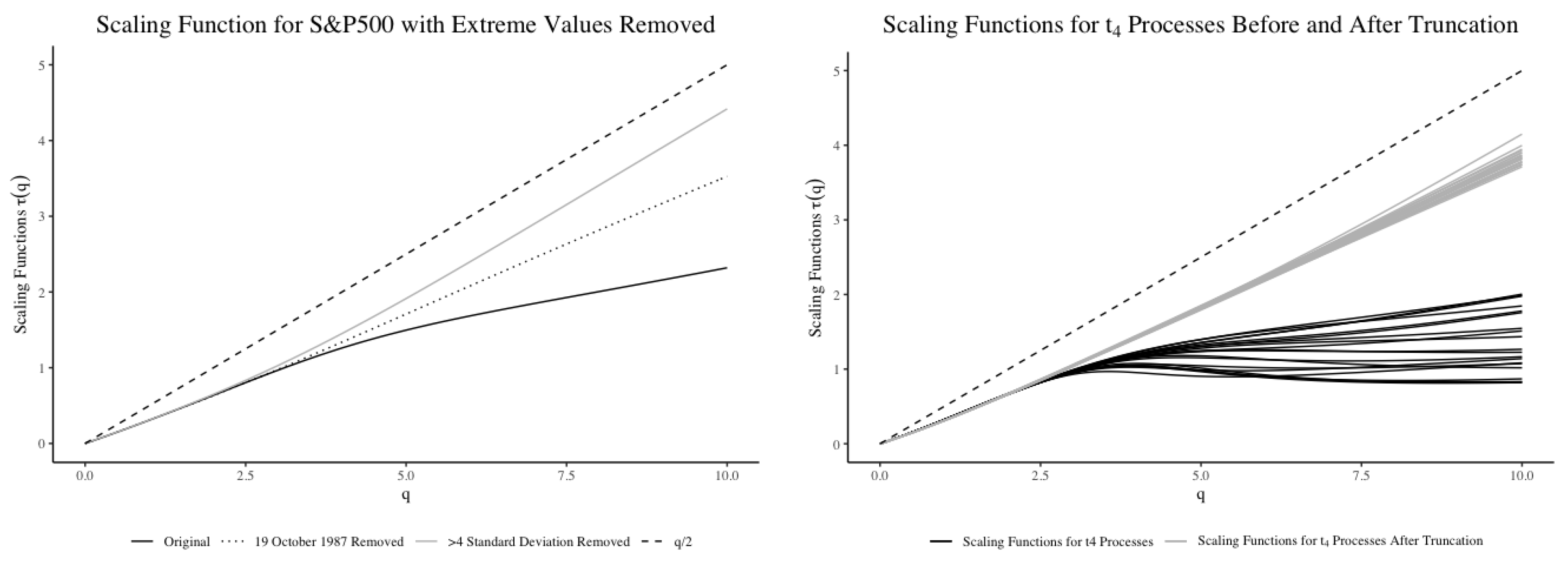
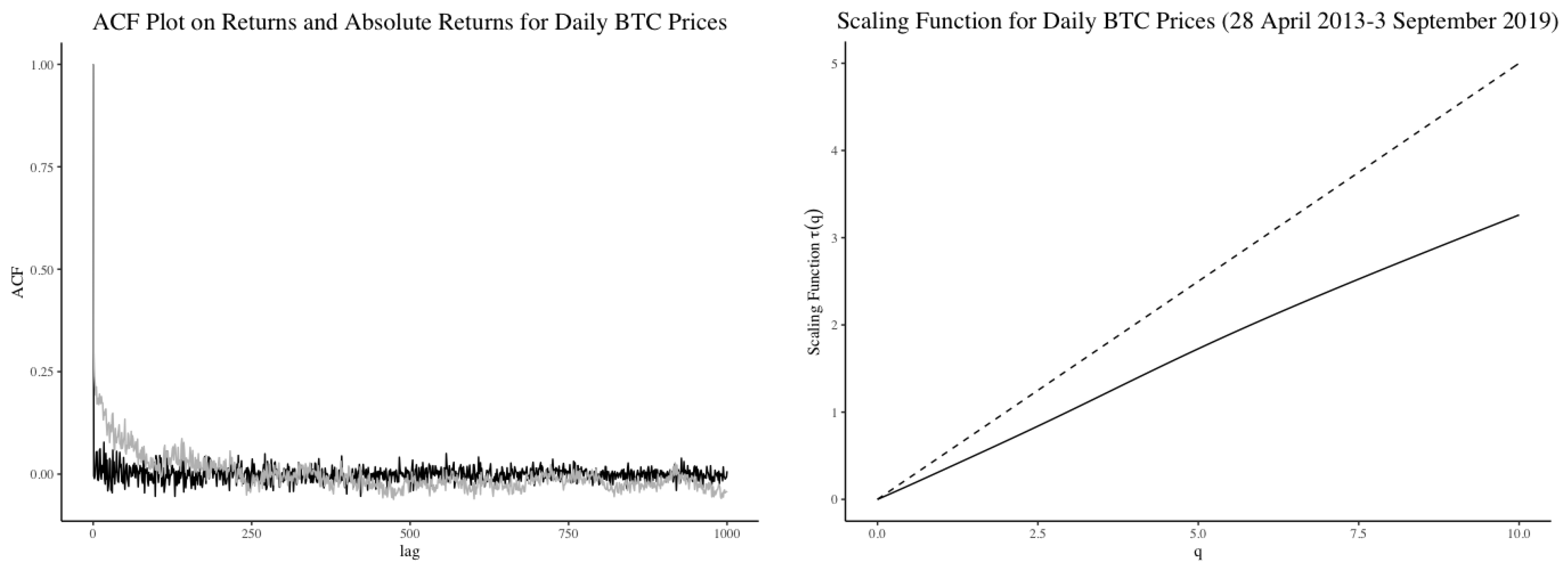
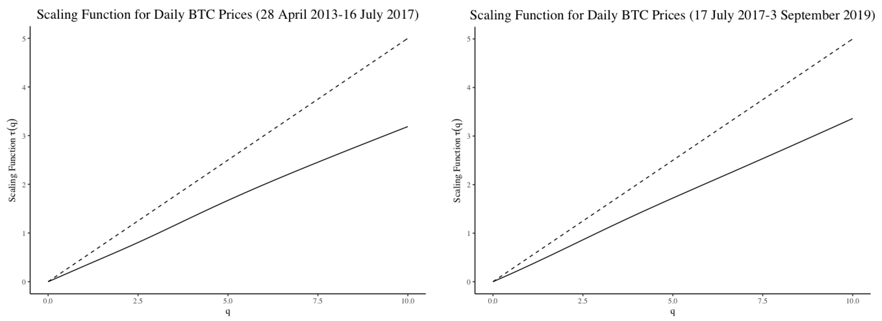
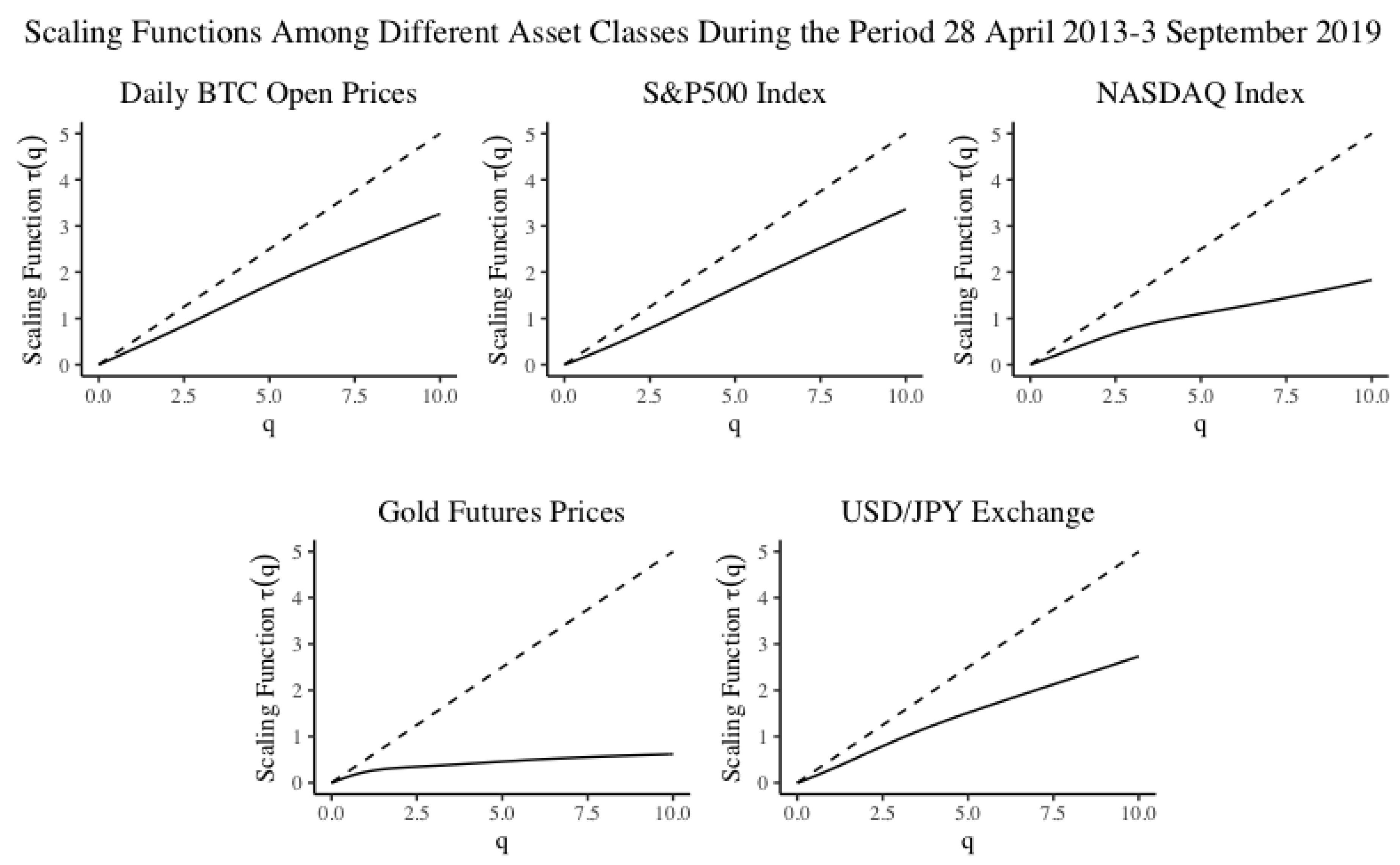
3.1. Application to Bitcoin

In this section, we apply our proposed hypothesis test to Bitcoin prices in order to address our research question: Do Bitcoin prices exhibit multifractal scaling? Both the global simplex statistic and the localised concavity measures are employed and reported. Two Bitcoin data sets are used in this paper:

• the daily Bitcoin open price, daily data (in USD) from 28 April 2013 to 3 September 2019 with 2,320 observations, retrieved from CoinMarketCap (2019); and
• the high frequency Bitcoin open price data minute-by-minute (in USDT) covering the period 22 May 2018 14:00 to 1 March 2019 11:00 with 406,089 observations, retrieved from Binance (2019).

Let $\left\{P\right(t),t=0,1,\dots ,T\}$ denote the open prices of Bitcoin. We define $X\left(t\right)$ to be the mean-centered log-prices

$$X\left(t\right)=lnP\left(t\right)-lnP\left(0\right)-\mu t,$$

where $\mu =\frac{1}{T}{\sum }_{i=1}^{T}ln\frac{P\left(i\right)}{P(i-1)}$. The mean-centered log-returns are then defined as

$$r\left(t\right)=X\left(t\right)-X(t-1).$$

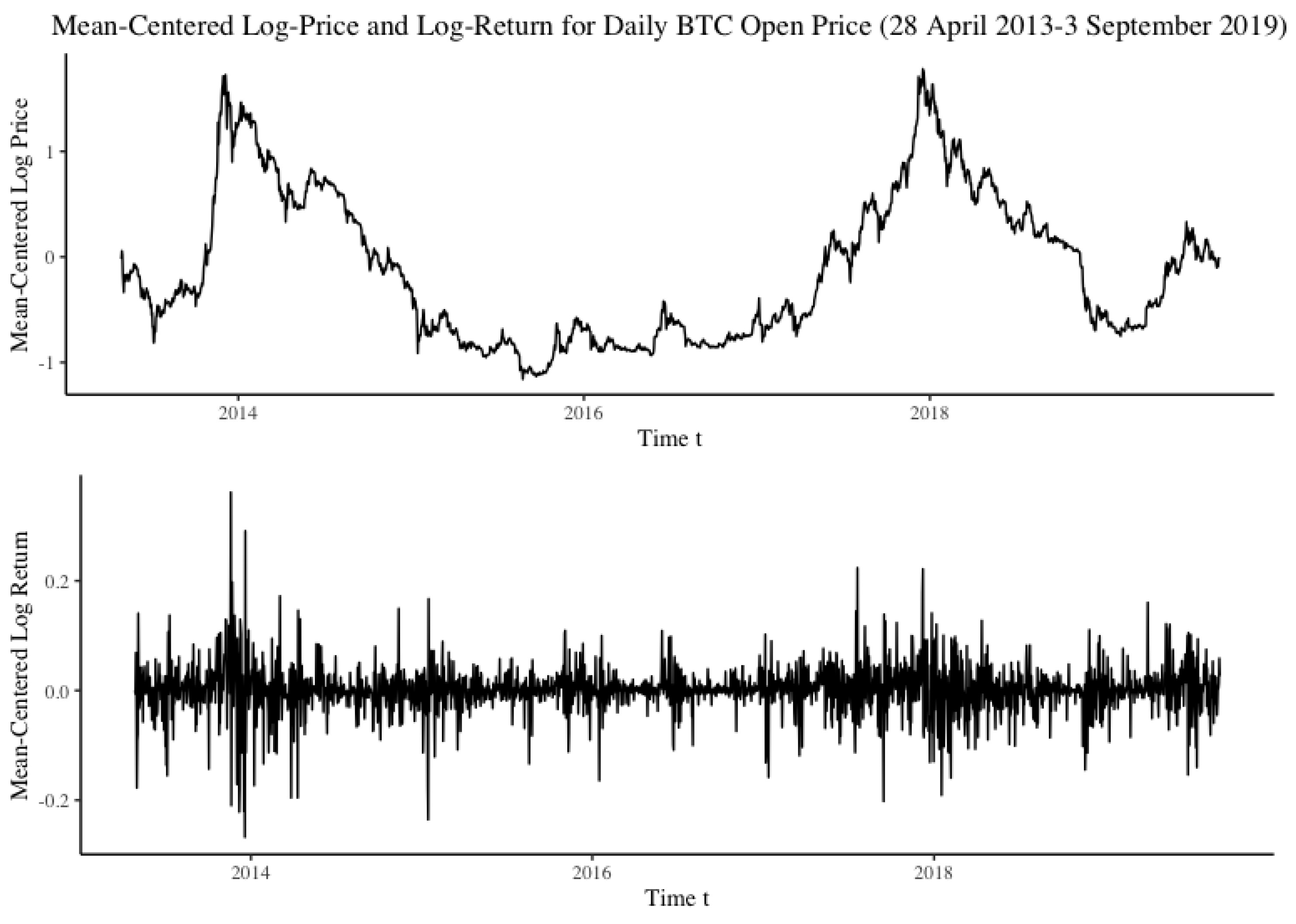
3.1.1. Daily Bitcoin Price Data

Mean-centered log-prices $X\left(t\right)$ and the log-returns for daily Bitcoin price are displayed in Figure 5. Two bull runs followed by two bear runs are observed in late 2013 and late 2017 represented by two prominent spikes. These two price surges are believed to be results of the increases in Bitcoin’s popularity and media coverage. A price drop is spotted in early 2018 followed by the price falls of most cryptocurrencies. This period is known as ‘the 2018 cryptocurrency crash’ (Popken 2018). The Bitcoin price collapsed by 80% from January to September 2018, which is reported to be worse than the dot-com bubble’s 78% collapse (Patterson 2018). Subsequently, a price hike on a smaller scale is observed between early 2019 and 3 September 2019.

A stylised feature check gives uncorrelated and stationary return increments but correlations in the absolute value of returns.

The estimation of $\tau \left(q\right)$ exhibits a relatively linear scaling function, as is shown in Figure 6. However, both concavity measures are less than 0, indicating the presence of concavity. A global simplex statistic of value $-0.2222$ and a localised concavity measure of value $-0.6256$ are obtained. The hypothesis tests based on these two measures indicate that the null hypothesis should be rejected in favour of the alternative; see

Table 1. Hypothesis test results on daily Bitcoin open prices (28 April 2013–3 September 2019).

Tail Index	3.0630
	Sample Size 1	Test Statistic	Rejection Region	Test Result
Localised Test	1479	$-0.2222$	$[-1,-0.0556)$	Multifractal
Global Test	99	$-0.6256$	$[-1,-0.6148)$	Multifractal

¹Sample size refers to the number of student t-distributed processes used in estimating the distribution of concavity measures under $H_0$. In the case of Bitcoin open prices from 28/04/2013 to 03/09/2019, there are 1479 student t-distributed processes with tail indices ranging in the interval [2.5630, 3.5630] when constructing the distribution of localised concavity measures. 99 student t-distributed processes are used in the construction of the distributions of global simplex statistics.

.

Thus, despite appearances in Figure 6, we have preliminary evidence that Bitcoin may follow a multifractal process.

To observe whether different results appear when the sample changes, the log-price time series is broken down into smaller time periods. The same hypothesis tests are performed to examine multifractality. Some literature indicates that 2017 is a turning point for Bitcoin’s price behaviour. Zhang et al. (2018) concluded an increase in market inefficiency from late 2016, which is believed to be a result of an increase in speculation. Consequently, we break the daily price process into two parts,

• $X_1\left(t\right)$ from 28 April 2013 to 16 July 2017 with 1541 observations; and,
• $X_2\left(t\right)$ from 17 July 2017 to 3 September 2019 with 779 observations.

The corresponding scaling functions are shown in Figure 7 with hypothesis test results in

Table 2. Hypothesis test results on daily Bitcoin open prices (28 April 2013–16 July 2017).

Tail Index	3.2791
	Sample Size	Test Statistic	Rejection Region	Test Result
Localised Test	1403	$-0.4444$	$[-1,-0.1111)$	Multifractal
Global Test	98	$-0.5378$	$[-1,-0.7014)$	Non-Multifractal

and

Table 3. Hypothesis test results on daily Bitcoin open prices (17 July 2017–3 September 2019).

Tail Index	1.6528
	Sample Size	Test Statistic	Rejection Region	Test Result
Localised Test	1992	$-0.8333$	$[-1,-0.6111)$	Multifractal
Global Test	75	$-0.9950$	$[-1,-0.8703)$	Multifractal

. The hypotheses tests for $X_1\left(t\right)$ give various results. This may be a result of a smaller data set or it could indicate a change to the way Bitcoin prices scale.

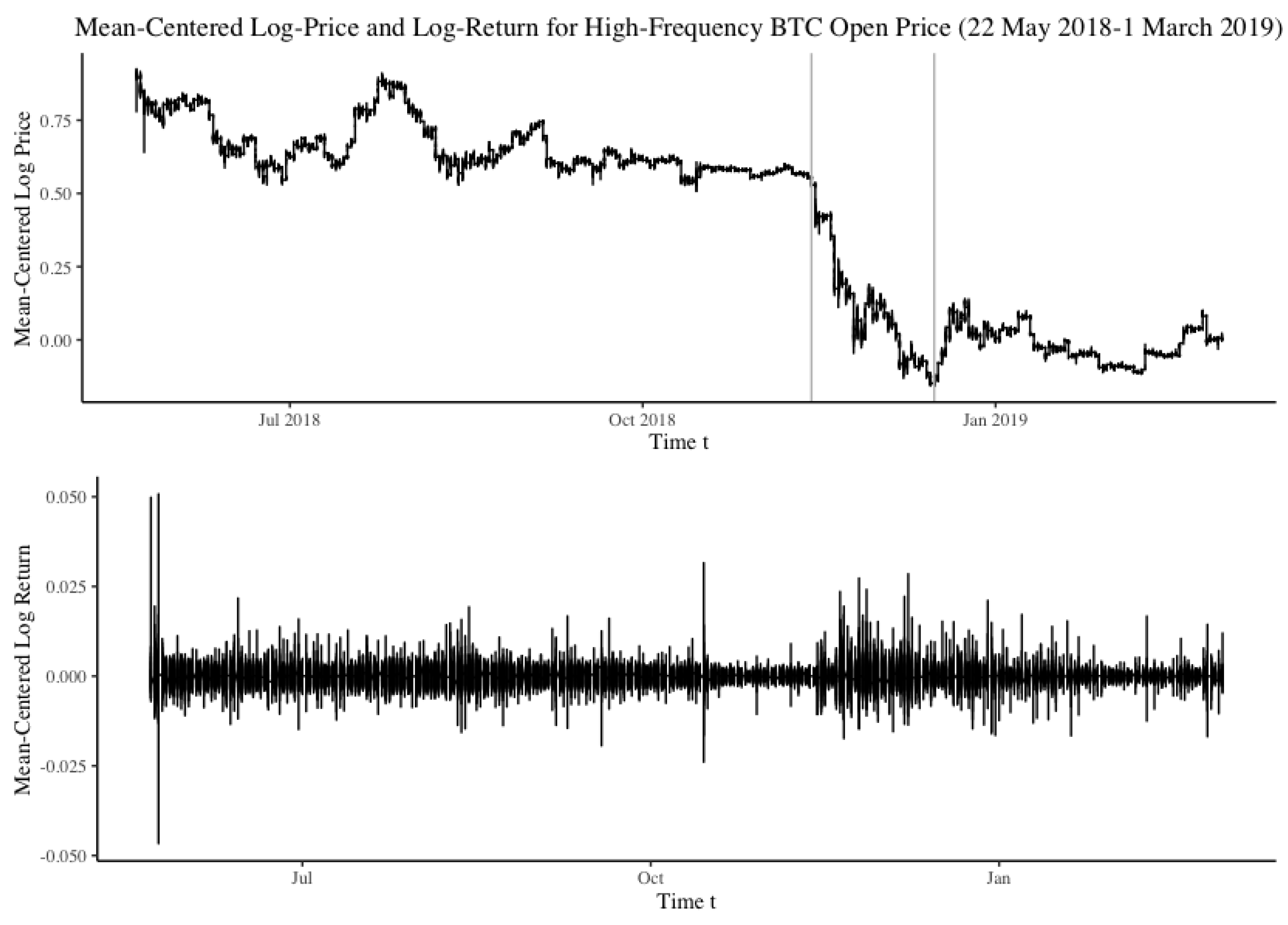
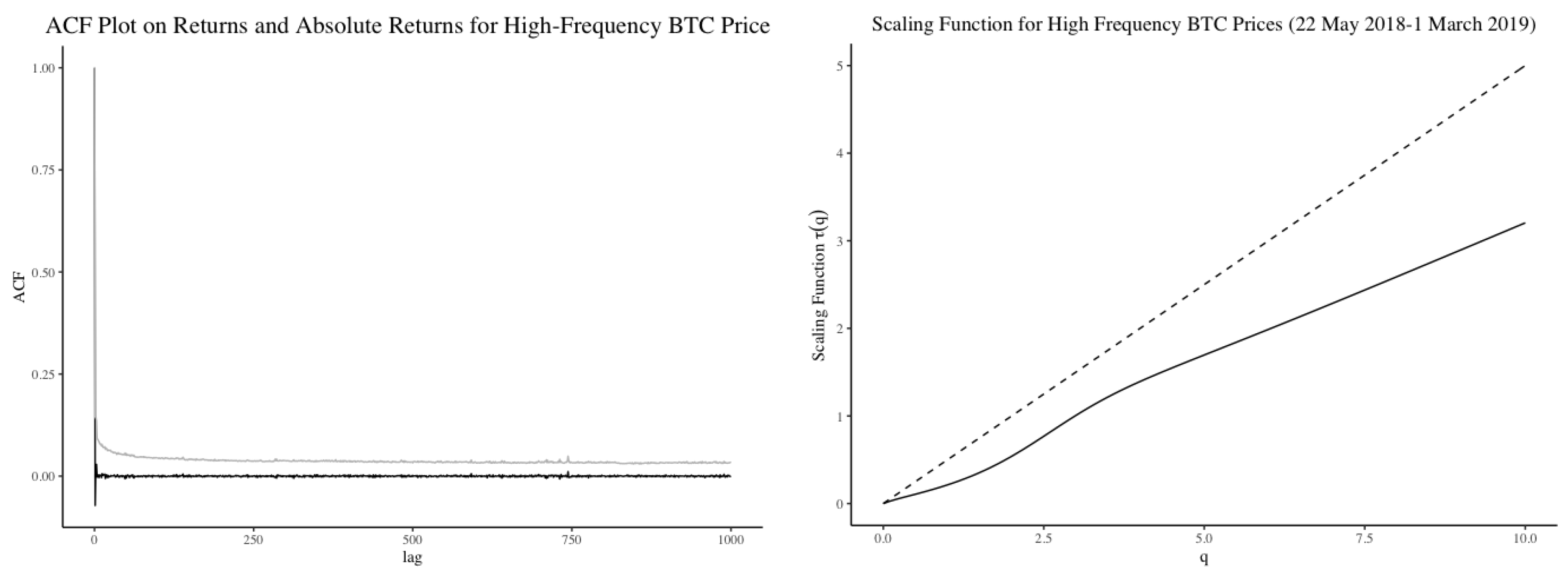
3.1.2. High-Frequency Bitcoin Price Data

Multifractality tests are performed on the high-frequency minute-by-minute data of Bitcoin open prices from 22 May 2018 14:00 to 1 March 2019 11:00 with 406,089 observations. Its mean-centered log-prices and log-returns are displayed in Figure 8. Similar to other financial assets, a lack of correlation in the return increments but high correlation in the absolute returns are found. However, compared with the daily open Bitcoin price data, the high-frequency Bitcoin data display stronger auto-correlation in the absolute return increments.

This data set covers approximately a one year period from May 2018 to March 2019. The two corresponding annual breakdown tests for daily Bitcoin open prices covering this period in Appendix B.1 in Appendix B do not indicate multifractal scaling, despite some evidence in Table 1 and Table 3 for multifractality in daily data, generally.

The analysis of the high-frequency minute-by-minute data are broadly consistent with this result. With the estimated scaling function $\widehat{\tau }\left(q\right)$ shown in Figure 9 and the test results in

Table 4. Hypothesis test results on high frequency Bitcoin open prices (22 May 2018–1 March 2019).

Tail Index	2.7759
	Sample Size	Test Statistic	Rejection Region	Test Result
Localised Test	1682	$0.2778$	$[-1,-0.0556)$	Non-multifractal
Global Test	83	$-0.2714$	$[-1,-0.5049)$	Non-multifractal

, there appears to be little evidence of multifractal scaling for the high frequency data. Nevertheless, as shown in Appendix B.2, multifractality can be detected in some cases if we partition the data into smaller subperiods.

Given these contradictory results and that the high-frequency data only spans one year, we are reluctant to infer at this stage that the Bitcoin time series scales in the same way over longer or shorter time intervals.

Overall, it is possible that multifractal scaling exists for Bitcoin prices; however, a longer time series is necessary to substantiate the use of a multifractal model and further tests are needed to discern between monofractal models as a parsimonious alternative. In the following section, we test for the presence of multifractal scaling in other financial assets. These assets have more established markets with a long history of price data. It is thus useful to compare their scaling properties to that of the Bitcoin and to identify any similarities.

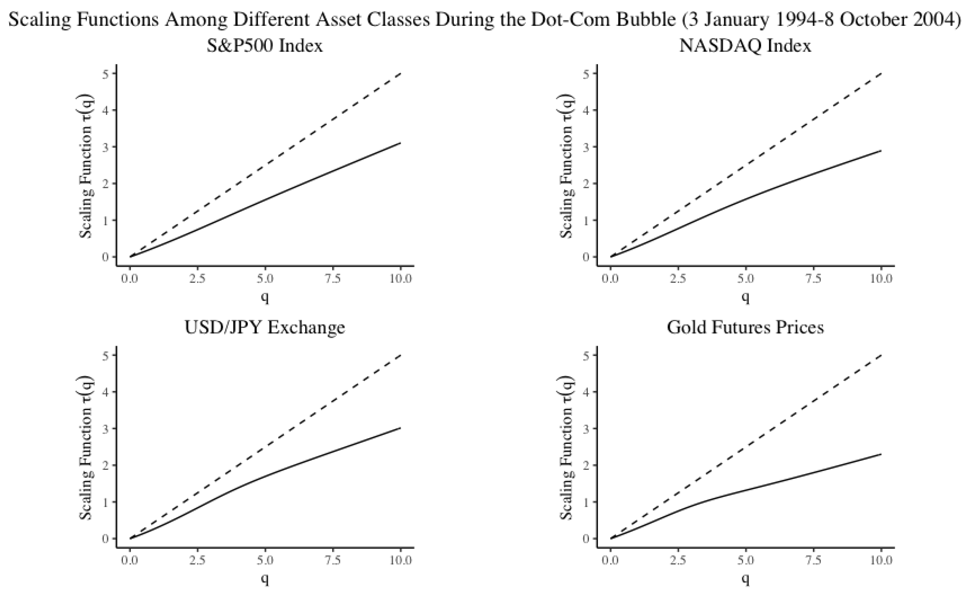
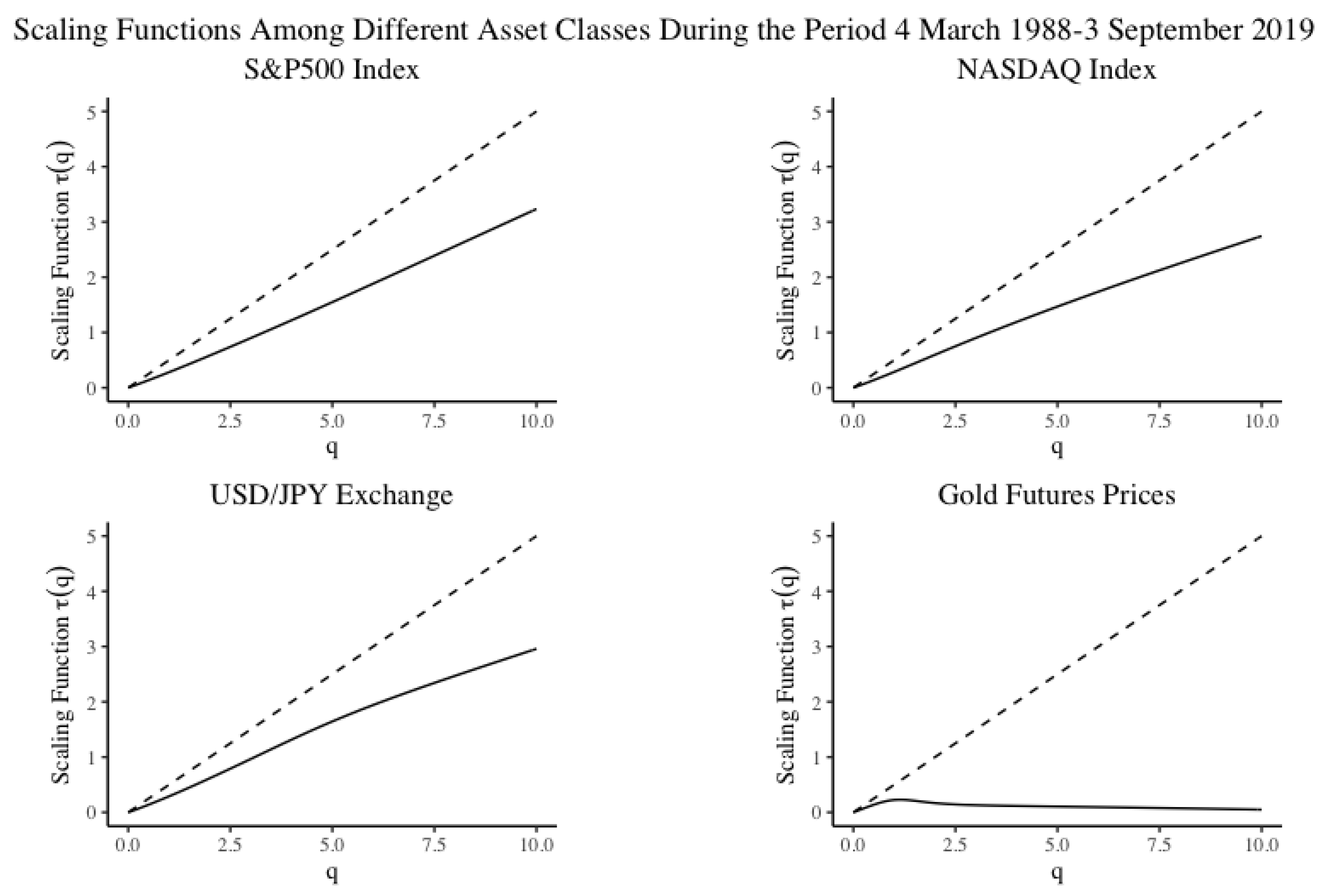
3.2. Bitcoin Compared to Other Financial Assets

Cryptocurrencies are a new financial asset whose value depends upon the evolution of its underlying technology as well as the design of its economic model. Bitcoin in particular appears to have characteristics that span a commodity, medium of exchange and technology. As a result, it is unclear which asset class Bitcoin most resembles. In the previous section, we identified that Bitcoin’s price dynamics could be characterised by multifractal scaling laws after accounting for heavy tails. In this section, we compare Bitcoin’s scaling properties to other financial assets. Included in our set of comparable assets are stock indices, a foreign exchange rate series and gold futures. The S&P500 index7 has been chosen to represent a large class of global equities; the Nasdaq Composite Index8 illustrates the price behaviour of technology-stocks; the USD/JPY exchange rate9 represents foreign currency; and gold futures prices10 are also included in the comparison, as Bitcoin is often referred to as the digital version of gold.

The results of the hypothesis tests are summarised in

Table 5. Test results among different financial assets (28 April 2013–3 September 2019).

Financial Asset	Tail Index	Test	Test Statistics	Rejection Region	Test Result (Local)
BTC Daily	3.06	Local	−0.22	[−1, −0.06)	Multifractal
		Global	−0.63	[−1, −0.61)	Multifractal
S&P500	3.13	Local	−0.11	[−1, −0.11)	Non-Multifractal
		Global	−0.14	[−1, −0.66)	Non-Multifractal
NASDAQ	3.19	Local	0.11	[−1, −0.11)	Non-Multifractal
		Global	−0.44	[−1, −0.66)	Non-Multifractal
USD/JPY	2.69	Local	−0.28	[−1, −0.17)	Multifractal
		Global	−0.86	[−1, −0.49)	Multifractal
Gold Futures	1.35	Local	−0.67	[−1, −0.72)	Non-Multifractal
		Global	−0.89	[−1, −0.9979)	Non-Multifractal

,

Table 6. Test results among different financial assets during the dot-com bubble (3 January 1994–8 October 2004).

Financial Asset	Tail Index	Test	Test Statistics	Rejection Region	Test Result (Local)
S&P500	3.41	Local	−0.22	[−1, −0.17)	Multifractal
		Global	−0.40	[−1, −0.71)	Non-Multifractal
NASDAQ	2.81	Local	−0.44	[−1, −0.06)	Multifractal
		Global	−0.79	[−1, −0.52)	Multifractal
USD/JPY	3.50	Local	−0.33	[−1, −0.17)	Multifractal
		Global	−0.80	[−1, −0.76)	Multifractal
Gold Futures	3.48	Local	0.22	[−1, −0.17)	Non-Multifractal
		Global	−0.48	[−1, −0.71)	Non-Multifractal

and

Table 7. Test results among different financial assets (4 March 1988–3 September 2019).

Financial Asset	Tail Index	Test	Test Statistics	Rejection Region	Test Result (Local)
S&P500	3.20	Local	0.78	[−1, −0.11)	Non-Multifractal
		Global	0.93	[−1, −0.66)	Non-Multifractal
NASDAQ	3.84	Local	−0.61	[−1, −0.22)	Multifractal
		Global	−0.93	[−1, −0.84)	Multifractal
USD/JPY	3.33	Local	−0.28	[−1, −0.17)	Multifractal
		Global	−0.72	[−1, −0.70)	Multifractal
Gold Futures	1.36	Local	−0.11	[−1, −0.72)	Non-Multifractal
		Global	0.11	[−1, −0.9979)	Non-Multifractal

and the associated scaling functions are depicted in Figure 10, Figure 11 and Figure 12. Table 5 compares Bitcoin daily prices to other assets, over a short time period spanning Bitcoin’s limited but available price history, from 2013–2019. We observe that the local and global results can produce conflicting evidence. The local test for the S&P500 marginally accepts the null hypothesis, where the global test result marginally accepts the alternative in favour of multifractality for BTC Daily. The global test statistic reveals that the greatest evidence for multifractal scaling is for the USD/JPY exchange series. The scaling functions for each asset class look visibly concave for all assets except the S&P 500; however, multifractality in the presence of heavy tails is only indicated for Bitcoin and the the USD/JPY, indicating on prima facie evidence that Bitcoin could share similar scaling properties to foreign exchange. However, Table 6 and Table 7 reveal more compelling evidence given the larger data set spanning longer time periods. The lengthy time period is able to capture scaling behaviour for a wide range of time scales, as is necessary to establish a multifractal scaling relationship for an arbitrary set of rescaling factors. The results in Table 6 and Table 7 indicate that both the NASDAQ and the USD/JPY foreign exchange series could share multifractal scaling properties along with Bitcoin. The scaling function of the Gold Futures series looks visibly concave; however, the hypothesis test accepts the null in the presence of heavy tails indicating that the concavity is a result of heavy tails as opposed to multifractal scaling.

4. Conclusions

Multifractal scaling cannot be assumed to exist a priori, but instead should be established after accounting for the heavy tail effect on scaling functions. In this paper, we demonstrate how one can develop a multifractal scaling hypothesis test that accounts for the heavy tail effect on scaling functions. The test outlined in this paper doesn’t incorporate the possibility of monofractal scaling, but it can be incorporated into the test in the future and we will undertake such an approach in further research. The hypothesis test presented in this paper distinguishes between the heavy tail effect that distorts a linear scaling function to look concave, and true multifractal scaling. To implement the test, a look-up table is employed to simplify the hypothesis test procedure. This makes it easy to implement the test on various time series with marginal distributions of varying tail indexes. Our test results are of course contingent upon the validity of the underlying distributional assumptions. While a sound statistical theory awaits further development, a thorough examination of the test properties by means of Monte Carlo simulation can be carried out straightforwardly, in future research.

We apply this hypothesis test to Bitcoin prices and reveal that Bitcoin exhibits scaling behaviour more similar to a multifractal model than to a heavy tail process. We then extend the test to a set of other financial assets to ascertain whether Bitcoin prices are likely to share multifractal scaling relationships akin to other financial time series. Our results show that Bitcoin, USD/JPY exchange rates, and the technology heavy NASDAQ could all share multifractal scaling properties, after accounting for heavy tails. The findings of this paper are that, while Bitcoin prices span a relatively short period, the hypothesis test indicates that multifractal scaling is plausible and such scaling could be a feature of foreign exchange markets and technology stocks as well. This indicates some helpful methodology for model selection in risk analysis. Furthermore, the research suggests that financial time series may be classified by their statistical scaling properties in addition to the asset class they belong to. This additional type of classification could allow practitioners to construct statistically diverse portfolios based on assets grouped by their scaling dynamics.

References

1. Abrevaya, Jason, and Wei Jiang. 2005. A nonparametric approach to measuring and testing curvature. Journal of Business & Economic Statistics 23: 1–19. [Google Scholar]
2. Bariviera, Aurelio F. 2017. The inefficiency of bitcoin revisited: A dynamic approach. Economics Letters 161: 1–4. [Google Scholar] [CrossRef] [Green Version]
3. Bariviera, Aurelio F., María José Basgall, Waldo Hasperué, and Marcelo Naiouf. 2017. Some stylized facts of the bitcoin market. Physica A: Statistical Mechanics and Its Applications 484: 82–90. [Google Scholar] [CrossRef] [Green Version]
4. Binance. 2019. BTC/USDT. Available online: https://www.binance.com/en/trade/BTC_USDT (accessed on 20 March 2019).
5. Bouchaud, Jean-Philippe, Marc Potters, and Martin Meyer. 2000. Apparent multifractality in financial time series. The European Physical Journal B-Condensed Matter and Complex Systems 13: 595–99. [Google Scholar] [CrossRef] [Green Version]
6. Calvet, Laurent E., Adlai J. Fisher, and Benoit B. Mandelbrot. 1997. Large Deviations and the Distribution of Price Changes. Cowles Foundation Discussion Paper No. 1165. New Haven: Cowles Foundation for Research in Economics Yale University. [Google Scholar]
7. Chambers, Clem. 2019. Bitcoin Is Fractal. Available online: https://www.forbes.com/sites/investor/2019/01/23/bitcoin-is-fractal/#27bbcc49208d (accessed on 30 April 2019).
8. CoinMarketCap. 2019. Bitcoin (BTC) Price, Charts, Market Cap, and Other Metrics. Available online: https://coinmarketcap.com/currencies/bitcoin/ (accessed on 5 September 2019).
9. Embrechts, Paul, and Makoto Maejima. 2000. An introduction to the theory of self-similar stochastic processes. International Journal of Modern Physics B 14: 1399–420. [Google Scholar] [CrossRef]
10. Grahovac, Danijel, and Nikolai N. Leonenko. 2014. Detecting multifractal stochastic processes under heavy-tailed effects. Chaos, Solitons & Fractals 65: 78–89. [Google Scholar]
11. Heyde, Chris C. 2009. Scaling issues for risky asset modelling. Mathematical Methods of Operations Research 69: 593–603. [Google Scholar] [CrossRef]
12. investing.com Australia. 2020a. Gold Futures—Apr 20 (GCJ0). Available online: https://au.investing.com/commodities/gold-historical-data (accessed on 27 February 2020).
13. investing.com Australia. 2020b. USD JPY Historical Data—Investing.com AU. Available online: https://au.investing.com/currencies/usd-jpy-historical-data (accessed on 27 February 2020).
14. Kantelhardt, Jan W., Stephan A. Zschiegner, Eva Koscielny-Bunde, Shlomo Havlin, Armin Bunde, and H. Eugene Stanley. 2002. Multifractal detrended fluctuation analysis of nonstationary time series. Physica A: Statistical Mechanics and Its Applications 316: 87–114. [Google Scholar] [CrossRef] [Green Version]
15. Lahmiri, Salim, and Stelios Bekiros. 2018. Chaos, randomness and multi-fractality in bitcoin market. Chaos, Solitons & Fractals 106: 28–34. [Google Scholar]
16. Mandelbrot, Benoit B., Adlai J. Fisher, and Laurent E. Calvet. 1997. A Multifractal Model of Asset Returns. Cowles Foundation Discussion Paper No. 1164. New Haven: Cowles Foundation for Research in Economics Yale University. [Google Scholar]
17. Matia, Kaushik, Yosef Ashkenazy, and H. Eugene Stanley. 2003. Multifractal properties of price fluctuations of stocks and commodities. EPL (Europhysics Letters) 61: 422. [Google Scholar] [CrossRef] [Green Version]
18. Mensi, Walid, Yun-Jung Lee, Khamis Hamed Al-Yahyaee, Ahmet Sensoy, and Seong-Min Yoon. 2019. Intraday downward/upward multifractality and long memory in bitcoin and ethereum markets: An asymmetric multifractal detrended fluctuation analysis. Finance Research Letters 31: 19–25. [Google Scholar] [CrossRef]
19. Milutinović, Monia. 2018. Cryptocurrency. Екoнoмика-Часoпис за екoнoмску теoрију и праксу и друштвена питањаа 1: 105–122. [Google Scholar] [CrossRef] [Green Version]
20. Nadarajah, Saralees, and Jeffrey Chu. 2017. On the inefficiency of bitcoin. Economics Letters 150: 6–9. [Google Scholar] [CrossRef] [Green Version]
21. Nakamoto, Satoshi. 2009. Bitcoin: A Peer-to-Peer Electronic Cash System. Available online: https://bitcoin.org/bitcoin.pdf (accessed on 20 November 2018).
22. Patterson, Michael. 2018. Crypto’s 80% Plunge Is Now Worse Than the Dot-Com Crash. Available online: https://www.bloomberg.com/news/articles/2018-09-12/crypto-s-crash-just-surpassed-dot-com-levels-as-losses-reach-80 (accessed on 7 August 2019).
23. Platen, Eckhard, and Renata Rendek. 2008. Empirical evidence on student-t log-returns of diversified world stock indices. Journal of Statistical Theory and Practice 2: 233–251. [Google Scholar] [CrossRef] [Green Version]
24. Popken, Ben. 2018. Bitcoin Loses More Than Half Its Value Amid Crypto Crash. Available online: https://www.nbcnews.com/tech/internet/bitcoin-loses-more-half-its-value-amid-crypto-crash-n844056 (accessed on 7 August 2019).
25. Salat, Hadrien, Roberto Murcio, and Elsa Arcaute. 2017. Multifractal methodology. Physica A: Statistical Mechanics and Its Applications 473: 467–487. [Google Scholar] [CrossRef]
26. Sly, Allan. 2006. Self-similarity, multifractionality and multifractality. Master’s thesis, Australian National University, Canberra, Australia. [Google Scholar]
27. Sreenivasan, Katepalli. 1991. Fractals and multifractals in fluid turbulence. Annual Review of Fluid Mechanics 23: 539–604. [Google Scholar] [CrossRef]
28. Stavroyiannis, Stavros, Vassilios Babalos, Stelios Bekiros, Salim Lahmiri, and Gazi Salah Uddin. 2019. The high frequency multifractal properties of bitcoin. Physica A: Statistical Mechanics and Its Applications 520: 62–71. [Google Scholar] [CrossRef]
29. Yahoo Finance. 2019. S&P 500 (^GSPC) Historical Data. Available online: https://au.finance.yahoo.com/quote/^GSPC/history?p=^GSPC (accessed on 27 February 2020).
30. Yahoo Finance. 2020. NASDAQ Composite (^IXIC) Historical Data. Available online: https://finance.yahoo.com/quote/%5Eixic/history?ltr=1 (accessed on 27 February 2020).
31. Zhang, Wei, Pengfei Wang, Xiao Li, and Dehua Shen. 2018. The inefficiency of cryptocurrency and its cross-correlation with dow jones industrial average. Physica A: Statistical Mechanics and Its Applications 510: 658–670. [Google Scholar] [CrossRef]
1.
“False positive” corresponds to the scenario that we mistakenly detect multifractality when the underlying process does not possess the multifractal property.
2.
For convenience, in the rest of this paper, we call uniscaling multifractal processes monofractal processes while referring to multiscaling multifractal processes as multifractal processes.
3.
We compared the scaling functions of the Bitcoin and other financial assets with the ones of BMMTs simulated using multiplicative cascades with Poisson distribution, Gamma distribution and Normal distribution. The scaling function of the BMMT simulated through log-Normal multiplicative cascade displays the most similar behaviour.
4.
The choice of Student’s t-distribution with 4 degrees of freedom is suggested by the findings of Platen and Rendek (2008).
5.
Knots were chosen so that the function is evaluated on 18 equal sub-intervals. This gave the best approximation considering computational efficiency.
6.
For example, if Hill’s estimator takes value h Hill = 2 , we generate simulated student t-distributed processes with 2 degrees of freedom, select those with tail indices in the interval [ 1.5 , 2.5 ] , and construct the null distribution using the empirical distribution of their concavity measures.
7.
Retrieved from Yahoo Finance (2019) for the period 30 December 1927 to 26 February 2020 with 23,147 observations.
8.
Retrieved from Yahoo Finance (2020) for the period 5 February 1971 to 25 February 2020 with 12,372 observations.
9.
Retrieved from investing.com Australia (2020b) for the period 4 March 1988 to 28 February 2020 with 8337 observations.
10.
Retrieved from investing.com Australia (2020a) for the period 27 December 1979 to 28 February 2020 with 10,190 observations.
Figure 1. Asymptotic scaling functions for various values of α . The grey line is the q / 2 reference line.
Jrfm 13 00104 g001
Figure 2. Left—Scaling Functions of the original S&P 500 open price data (black solid line), the S&P 500 open price data after removing 19 October 1987 (dotted line), the S&P 500 open price data after truncating any return larger than 4 standard deviations from the mean (grey solid line). Right—Scaling Functions of the Student t-distributed processes before (black lines) and after truncation (grey lines). For comparison, the reference lines q / 2 (black dashed line) are included.
Jrfm 13 00104 g002
Figure 3. Distribution of global simplex statistics for Brownian motion (left) and fractional Brownian motion (right).
Jrfm 13 00104 g003
Figure 4. Distributions of global simplex statistics for Student t-distributed process (black) and the simulated BMMT with log-normal multiplicative cascade (grey) around tail index 3.06. The two vertical lines represent the 95th percentile for the simulated BMMTs (left) and 5th percentiles for the Student t-distributed processes, respectively (right).
Jrfm 13 00104 g004
Figure 5. Daily mean-centered log Bitcoin open price process (top) and mean-centered log returns process (bottom).
Jrfm 13 00104 g005
Figure 6. Left—Autocorrelations of mean-centered log-returns (black) and absolute returns (grey) for daily Bitcoin open price (28 April 2013–3 April 2019). Right—Scaling function for daily Bitcoin open price (28 April 2013–3 September 2019). The dashed line is the q / 2 reference line (same for all the scaling function figures).
Jrfm 13 00104 g006
Figure 7. Scaling functions for Daily Bitcoin open price from 28 April 2013 to 16 July 2017 (left) vs. from 17 July 2017 to 3 September 2019 (right).
Jrfm 13 00104 g007
Figure 8. High frequency mean-centered log Bitcoin open price process (top) and mean-centered log returns process (bottom).
Jrfm 13 00104 g008
Figure 9. Left—Autocorrelations of mean-centered log returns (black) and absolute returns (grey) for high frequency Bitcoin open prices (22 May 2018–1 March 2019). Right—Scaling function for high frequency Bitcoin open prices (22 May 2018–01 March 2019).
Jrfm 13 00104 g009
Figure 10. Scaling functions for S&P500, NASDAQ Index, USD/JPY Exchange and Gold Futures Prices the period 28 April 2013 to 3 September 2019.
Jrfm 13 00104 g010
Figure 11. Scaling functions for S&P500, NASDAQ Index, USD/JPY Exchange and Gold Futures Prices during the dot-com bubble (3 January 1994–8 October 2004). The time period from 3 January 1994 to 8 October 2004 corresponds to the dot-com bubble and the dot-com crash.
Jrfm 13 00104 g011
Figure 12. Scaling functions for S&P500, NASDAQ Index, USD/JPY Exchange and Gold Futures Prices the period 4 March 1988 to 3 September 2019.
Jrfm 13 00104 g012