Remarks on Bank Competition and Convergence Dynamics

Abstract

In a recent paper, Karadima and Louri use frontier-based measures of market power and bank competition in an application to Euro Area banking. The purpose of the present note is to access their paper in a critical way, as there are certain fallacies and errors.

Main Points of Criticism

The purpose of this note is to clear up some confusion regarding market power, the Lerner index and estimation of marginal cost. Karadima and Louri (2020, KL), for example, state that: “In our study, bank market power is measured by the Lerner index (L), which identifies the degree of monopoly power as the difference between the price (P) of a firm and its marginal cost (MC) at the profit-maximizing rate of output”, viz:

$$L=\frac{P-MC}{P}.$$

(1)

KL state incorrectly that: “The traditional approach of first estimating Equation (3) and then using the derived coefficient values to calculate marginal cost (MC) is based on the unrealistic assumption that all firms are profit maximizers”. However, it is clear that if a cost function is estimated as in their Equation (3), then the only behavioral assumption involved is cost minimization, not profit maximization, and this assumption is, of course, fairly weak.

In turn, KL following Kumbhakar et al. (2012) estimate a “return-to-dollar” specification (Equation (7)) to derive a measure of mark up. To understand the methodology, suppose we have a single output, $Q$. Since $P>MC=\frac{\partial C}{\partial Q}$, we can write this equivalently as

$$P>\frac{\partial ln C}{\partial ln Q}\cdot \frac{C}{Q}\Rightarrow \frac{TR}{C}>E_{CQ},$$

(2)

where $E_{CQ}$ is the output cost elasticity, and total revenue is $TR=pQ$. Moreover $r=\frac{TR}{TC}$ is the return to dollar (revenue per unit cost). From this analysis, they proceed to estimate

$$r_t=E_{CQ,t}+v_t+u_t$$

(3)

where $r_t=\frac{T{R}_t}{C_t}$, $v_t$ is statistical noise and $u_{it}\ge 0$ is a non-negative random variable that can be related to mark up as

$${\mathsf{\Theta }}_t\equiv \frac{P_t-M{C}_t}{M{C}_t}=\frac{u_t}{E_{CQ,t}},$$

(4)

from which the Lerner index is computed as

$$L_t=\frac{{\Theta }_t}{1+{\Theta }_t}.$$

(5)

Clearly, KL did not estimate a cost function as claimed but rather a return-to-dollar specification, as in their Equation (7): “Using the maximum likelihood method, Equation (7) is estimated separately for each country in order to account for different banking technologies per country. The estimation procedure is based on the distributional assumption that the non-negative term $u_t$ is independently half-normally distributed [...] while v_i is independently normally distributed [...]” (page 9).

It is not clear why one would want the return-to-dollar function in their Equation (7), as we can easily show the following:

$$L=\frac{P-MC}{P}=\frac{P-\frac{\partial C}{\partial Q}}{P}=\frac{P-\frac{\partial ln C}{\partial ln Q}\cdot \frac{C}{Q}}{P}=\frac{r-E_{CQ}}{r}.$$

(6)

Thus, the Lerner index depends exclusively on the output cost elasticity ($E_{CQ}$) and return-to-dollar ($r$). Therefore, it would suffice to estimate the cost function in their Equation (3), as they state on page 7 and in the discussion surrounding their Equation (2). As a matter of fact, estimating their (7) ignores the restrictions imposed by the cost function in (2) or (3).

Moreover, their $\mathsf{\Theta }\equiv \frac{P-MC}{MC}$ is, in fact, equal to

$$\mathsf{\Theta }=\frac{P-MC}{MC}=\frac{P-\frac{\partial C}{\partial Q}}{\partial C/\partial Q}=\frac{P-\frac{\partial ln C}{\partial ln Q}\cdot \frac{C}{Q}}{\frac{\partial ln C}{\partial ln Q}\cdot \frac{C}{Q}}=\frac{r-E_{CQ}}{E_{CQ}}=\frac{r}{E_{CQ}}-1$$

(7)

Our (6) and (7) are, of course, equivalent, and it follows immediately that $L=\frac{\mathsf{\Theta }}{1+\mathsf{\Theta }}$. Therefore, the question is: Why would one want to estimate a return-to-dollar specification as in KL Equation (7), ignoring the cost function, from which one can obtain directly $E_{CQ}$? One answer is that we have $\mathsf{\Theta }=\frac{u}{E_{CQ}}$, which incorporates the one-sided error term, but this is equivalent (up to statistical noise) to our Equation (7).

Moreover, KL use as a proxy for $Q$ the value of total assets but also mention that “In contrast to $P$, the value of MC is not directly observable”. However, the original motivation in Kumbhakar et al. (2012) was that precisely $P$ is often not available. Moreover, KL write that “$P$ is defined as the ratio of total revenues (total interest and non-interest income) to total assets so, in fact, it is not the “price of output” but rather it is $r$. In turn, presumably, they take the estimate of the one-sided error component in the return-to-dollar specification when the dependent variable is $r$, which is clearly wrong in view of our (6) and (7).

It must also be pointed out that the methodology of Kumbhakar et al. (2012) was developed for industries that produce a single homogeneous product. However, the multi-output nature of production in banking is well understood, and use of a single output is a serious misspecification (see Malikov et al. 2016 and their cited references). The correct procedure would have been to define carefully the different outputs and derive mark ups for each one of them as, presumably, banks are competing in different markets for different outputs. Therefore, the different Lerner indices for outputs $Q_1,\dots ,Q_M$ would have been

$$L_m=\frac{r_m-E_{CQ,m}}{E_{CQ,m}}, m=1,\dots ,M,$$

(8)

where $E_{CQ,m}=\frac{\partial ln C}{\partial ln Q_m}$ ($m=1,\dots ,M$). Even in the single-output case, it is unclear whether $u$ correctly measures market power. As $P>MC$, one can write this as $P=MC+V+U$ where $V$ stands for statistical noise and $U$ is another non-negative random variable. After a little algebra, we obtain:

$$r=E_{CQ}+\frac{V+U}{AC},$$

(9)

where $AC=\frac{C}{Q}$ is average cost. Whether one should estimate (9) or a return-to-dollar as in KL Equation (7) is unclear and depends on the researcher’s preferences. If, in fact, (9) is the correct way to proceed, then Equation (7) in KL is misspecified as the composed error ($E\equiv V+U$) is multiplied by the inverse of average cost and is, therefore, heteroskedastic. A battery of tests can be then be provided to convince the reader that KL’s (7) is better than (9).

However, there is an additional mistake in KL. In their Equation (14), they attempt to test for convergence in the “level of competition” ($C_{it}$), defined as the inverse of the Lerner index, viz. $C_{it}=\frac{1}{L_{it}}$. Their Equation (14) is as follows:

$$\ln \frac{C_{it}}{C_{i,t-1}}={\mu }_i+\beta \ln C_{i,t-1}+{\epsilon }_{it},$$

(10)

where ${\mu }_i$ denotes fixed effects, and ${\epsilon }_{it}$ is an error term. It is easy to show that

$$C_{it}=\frac{E_{CQ,it}+{\widehat{u}}_{it}}{{\widehat{u}}_{it}},$$

(11)

where ${\widehat{u}}_{it}$ is the familiar Jondrow et al. (1982) estimate of $u_{it}$ in the return-to-dollar function. If we omit the caret, we can write (10) as follows.

$$\ln \frac{C_{it}}{C_{i,t-1}}={\mu }_i+\beta \left[\ln \left(E_{CQ,i,t-1}+u_{it}\right)-\ln u_{i,t-1}\right]+{\epsilon }_{it},$$

(12)

from which follows

$$\ln \left(E_{CQ,it}+u_{it}\right)-\ln \left(E_{CQ,i,t-1}+u_{i,t-1}\right)+\ln u_{i,t-1}-\ln u_{i,t}={\mu }_i+\beta \left[\ln \left(E_{CQ,i,t-1}+u_{it}\right)-\ln u_{i,t-1}\right]+{\epsilon }_{it}.$$

(13)

Although further simplification is possible, it is clear from this formulation that there is a serious problem. A researcher that attempts to estimate markups ($u_{it}$) in order to test for convergence in a model like (13) reveals implicitly that she believes $u_{it}$ is autocorrelated. But this assumption is clearly inconsistent with the assumption that $u_{it}$ was assumed to be independent and identically distributed (IID) in the return-to-dollar formulation. Therefore, parameter estimates in both the return-to-dollar equation as well as in (13) will be biased and inconsistent.

Another problem with this formulation is that around $E_{CQ,it}\simeq 1$, using the approximation $\ln (1+u)\simeq u$, from (13), we obtain:

$$u_{it}-\ln u_{it}={\mu }_i+\rho \left(u_{i,t-1}-\ln u_{i,t-1}\right)+{\xi }_{it},$$

(14)

where $\rho =1+\beta$, and ${\xi }_{it}$ is a new error term that includes ${\epsilon }_{it}$ as well as approximation errors from the assumption that $E_{CQ,it}\simeq 1$ and the assumption that $u_{it}$ is small enough to justify a Taylor expansion of $\ln (1+u_{it})$. Therefore, at least approximately, “convergence regressions” based on KL’s formulation in (12) imply a strong prior belief about autocorrelation in $u_{it}$ as in (14). Again, the initial assumption that $u_{it}$ was IID and the latter assumption in (14) are logically inconsistent, thus leading to biased and inconsistent parameter estimators in both the return-to-dollar function (Equation (7) in KL) and the “convergence equation” in (10). If anything, and at best, estimates of $\beta$ can be used to diagnose whether the return-to-dollar specification is correct. From Table 7 in KL, we see that estimates of $\beta$ are fairly close to −1, but they are highly statistically significant. Thus, $1+\beta$ is close to zero but highly significant, implying autocorrelation in $u_{it}$s based on (14). Therefore, since (14) is correct, the initial IID assumption must be wrong and all estimates are biased and inconsistent.

To illustrate, we use the US banking data set in Malikov et al. (2016) where we have five input prices and five outputs, and we include log equity as a quasi-fixed input along with a time trend.1

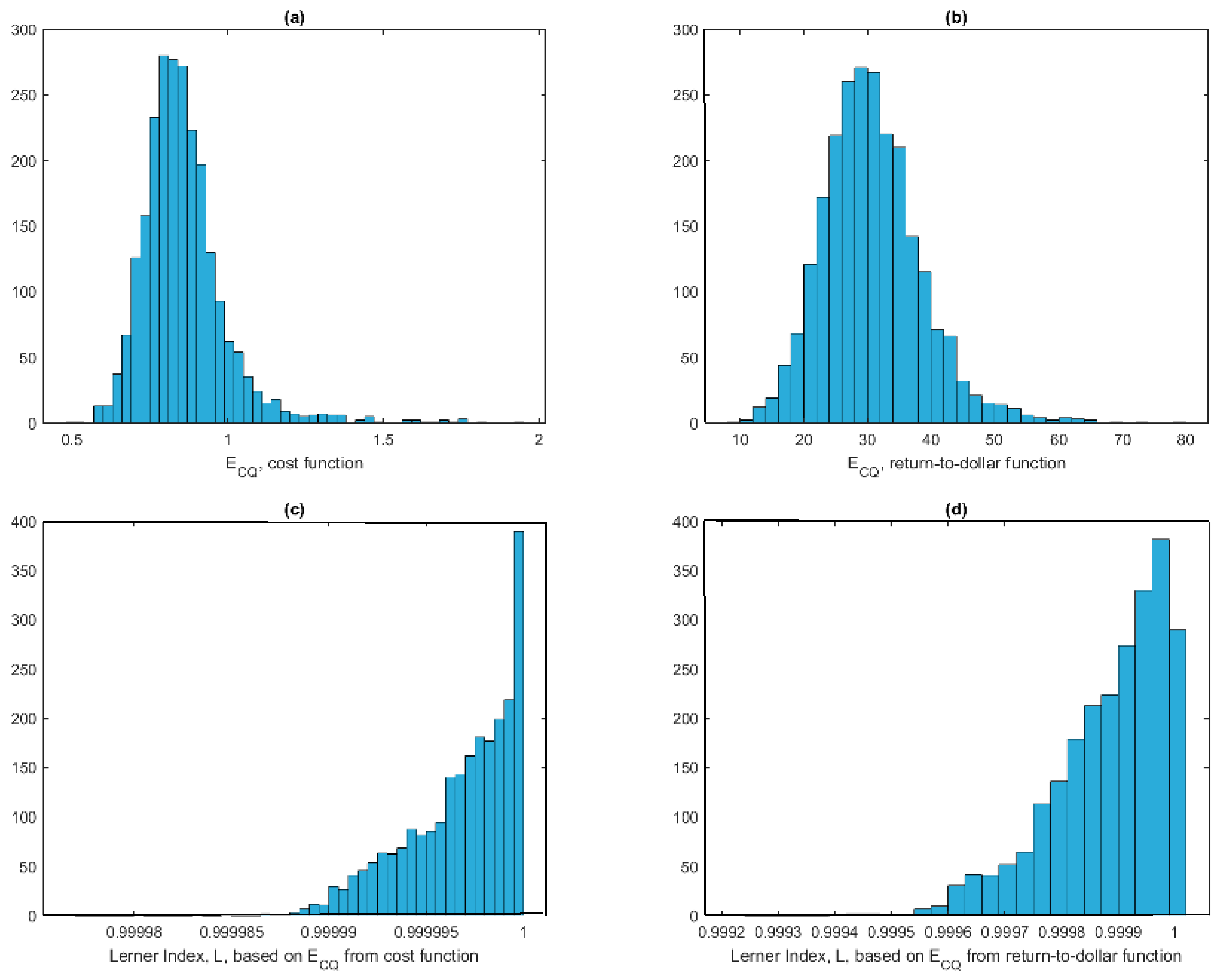
In panels (a) and (b) of Figure 1, we report estimates of $E_{CQ}$ (using the same single output $Q$ as in KL) from a translog cost function and the return-to-dollar specification. Quite clearly, $E_{CQ}$ estimates from the latter are non-sensical, whereas estimates from the cost function itself are quite reasonable. Lerner indices computed using the estimates of $E_{CQ}$ as in KL are reported in panels (c) and (d) of Figure 1 and they make little sense as well.

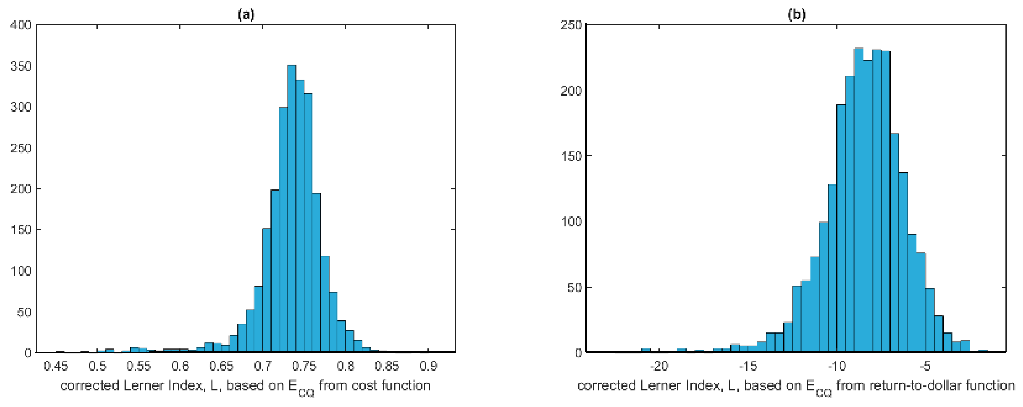
In an attempt to remedy the problem, we report, in Figure 2, corrected Lerner indices based on the formula $L=1-\frac{E_{CQ}}{r}$ where, again, $E_{CQ}$ is computed as in KL using either the cost function (panel (a)) or the return-to-dollar function (panel (b)). Although the estimates in panel (a) make sense, the Lerner indices reported in panel (b), which are based on estimating $E_{CQ}$ from the return-to-dollar function, make no sense at all, as they are all negative!

References

- Jondrow, James, C. A. Knox Lovell, Ivan S. Materov, and Peter Schmidt. 1982. On the estimation of technical inefficiency in the stochastic frontier production function model. Journal of Econometrics 19: 233–38. [Google Scholar] [CrossRef] [Green Version]
- Karadima, Maria, and Helen Louri. 2020. Bank Competition and Credit Risk in Euro Area Banking: Fragmentation and Convergence Dynamics. Journal of Risk and Financial Management 13: 57. [Google Scholar] [CrossRef] [Green Version]
- Kumbhakar, Subal C., Sjur Baardsen, and Gudbrand Lien. 2012. A new method for estimating market power with an application to Norwegian sawmilling. Review of Industrial Organization 40: 109–29. [Google Scholar] [CrossRef]
- Malikov, Emir, Subal C. Kumbhakar, and Mike G. Tsionas. 2016. A Cost System Approach to the Stochastic Directional Technology Distance Function with Undesirable Outputs: The Case of U.S. Banks in 2001–2010. Journal of Applied Econometrics 31: 1407–29. [Google Scholar] [CrossRef] [Green Version]