Efficient Numerical Pricing of American Call Options Using Symmetry Arguments

Abstract

This paper demonstrates that it is possible to improve significantly on the estimated call prices obtained with the regression and simulation-based least-squares Monte Carlo method by using put-call symmetry. The results show that, for a large sample of options with characteristics of relevance in real-life applications, the symmetric method performs much better on average than the regular pricing method, is the best method for most of the options, never performs poorly and, as a result, is extremely efficient compared to the optimal, but unfeasible method that picks the method with the smallest Root Mean Squared Error (RMSE). A simple classification method is proposed that, by optimally selecting among estimates from the symmetric method with a reasonably small order used in the polynomial approximation, achieves a relative efficiency of more than $98\%$. The relative importance of using the symmetric method increases with option maturity and with asset volatility. Using the symmetric method to price, for example, real options, many of which are call options with long maturities on volatile assets, for example energy, could therefore improve the estimates significantly by decreasing their bias and RMSE by orders of magnitude.

1. Introduction

In a paper published some 20 years ago, McDonald and Schroder (1998) demonstrated that when the price of the underlying asset is governed by a Geometric Brownian Motion (GBM), the price of a call option with underlying asset price S, strike price K, interest rate r and dividend yield d is equal to the price of an otherwise identical put option with asset price K, strike price S, interest rate d and dividend yield r. The result for the GBM case has since been generalized to more realistic dynamics in (Schroder 1999), among others, and essentially, some version of this Put-Call Symmetry (PCS), potentially with other fundamental parameters changed accordingly, will hold for virtually all the models that have been considered in the existing literature on option pricing, for options with several different payoffs and which are written on multiple assets.1

In this paper, we show that this simple result can be used to improve on one of today’s state-of-the-art numerical option pricing methods, the well-known Least-Squares Monte-Carlo (LSMC) method proposed by Longstaff and Schwartz (2001). In particular, we show that using PCS with LSMC results in estimates that are much less biased and have significantly lower Root Mean Squared Error (RMSE) when pricing American call options for the set of options used in (Longstaff and Schwartz 2001) and for a very large sample of options with realistic characteristics. Using standard choices for the LSMC method, which we implement with $N=$ 100,000 paths and a polynomial of order $L=3$, we price options with different strike prices and maturities in a world with different values for the interest rate, dividend yield and volatility. For a large sample of 3125 different options, the average RMSE of the estimates obtained with the symmetric method is only $17\%$ of the RMSE of the estimates from the regular method, and the symmetric estimates have smaller RMSEs for $88\%$ of the options in the sample.

Our results show that the relative performance of the symmetric method, i.e., when call options are priced as put options using PCS, improves as the time to maturity and volatility increase. Moreover, using the symmetric method is most effective for options that are out of the money. The simple intuition for this results is that when option maturity is long and volatility is high, asset values along simulated paths may become “very” large and be spread out over a large interval. Large and widely-spread out asset values lead to poorly-conditioned cross-sectional regressions and this in terms results in poor approximations of the optimal early exercise strategy and precisely determining this strategy is most important for out of the money options. Widely-dispersed asset values also lead to estimates that have higher variance because of the spread out payoffs being discounted back to estimate the price.

The magnitude of the relative improvement obtained with the symmetric method depends on the choice of parameters used in the LSMC algorithm, that is the number of simulated paths, N, and the number of regressors used in the cross-sectional regression, L, in a non-trivial way. In particular, while it is well known (see for example Stentoft (2004b)) that the option price estimated with the LSMC converges to the true value when the number of paths and the number of regressors tend to infinity, this is of little use with finite choices of the number of paths, N, and the order of the polynomial used in the regression, L. However, even with the “worst possible” configuration for the symmetric method, which occurs when $N=$ 100,000 and $L=5$ where the symmetric method only performs the best for roughly $39\%$ of the individual options, the average RMSE is much smaller than for the regular method and only $18\%$ larger than what could have been obtained with an infeasible method that picks from the regular and symmetric method the one with the smallest RMSE.

One reason that the choice of polynomial is important is that the LSMC method mixes two types of biases: a low bias due to having to approximate the optimal stopping time with a finite degree polynomial and a high bias coming from using the same paths to determine the optimal early exercise strategy and to price the option, potentially leading to over fitting to the simulated paths. For example, the bias just happens to be somewhat smaller without symmetry, a value of $-0.006$, than when using symmetry, a value of $0.010$ when using $L=5$ regressors with $N=$ 100,000 paths. For all other choices of the number of paths with this number of regressors and when using other numbers of regressors with this number of simulated paths, the symmetric estimates are less biased. An easy way to control the bias is to conduct so-called out-of-sample pricing in which a new set of simulated paths is used to price the option instead of using the same set of paths used for determining the optimal early exercise strategy.

When using out-of-sample pricing, the relative importance of the symmetric method is even more striking. In particular, the symmetric method almost always, and in some cases for more than $99\%$ of the individual options, has the lowest RMSE, and the average RMSE for the large sample of options is around $20\%$ or less of what is obtained with the regular method for most configurations. The efficiency of the symmetric method, when compared to the infeasible optimal method, is extraordinary and in most cases above $99\%$ across various values of the number of paths, N, and number of regressors, L, whereas the regular method only achieves an efficiency of around $25\%$. Finally, while it is difficult to pick the best method in general, in the case of out of sampling pricing, we propose a simple classification algorithm that, by optimally selecting among estimates from the symmetric method with a reasonably small order used in the polynomial approximation, achieves a relative efficiency of more than $98\%$ compared to the infeasible method that minimizes the RMSE across all estimates.

As noted by Detemple (2001), PCS is a useful property of many option pricing models since it reduces the computational burden when implementing these model. Indeed, a consequence of the property is that the same numerical algorithm can be used to price put and call options and to determine their associated optimal exercise policy. Another benefit is that it reduces the dimensionality of the pricing problem for some payoff functions. Examples include exchange options or quanto options. PCS also provides useful insights about the economic relationship between derivatives contracts. Puts and calls, forward prices and discount bonds and exchange options and standard options are simple examples of derivatives that are theoretically closely connected by symmetry relations. Compared to this literature, our objective is somewhat different. In particular, though PCS can be used to demonstrate theoretically the convergence of a particular numerical scheme for call option pricing using results for put options, our interest here is primarily of a numerical nature, and the objective is to show that PCS can be used to improve significantly on the estimated call option prices obtained with a particular numerical scheme.2

Our findings and proposed method for selecting optimally the configuration to use for option pricing should have broad implications. In particular, we show that improvements are found for a very large sample of options with reasonable characteristics, and since the symmetric method never performs very poorly and simple classification methods can be used to achieve very high relative efficiency, there are strong arguments for always using the symmetric method to price call options. Moreover, our results show that the relative importance of using the symmetric method increases with option maturity and asset volatility, and using symmetry to price long-term options in high volatility situations thus improves massively on the price estimates. The LSMC method is routinely used to price real options, most of which are call options with long maturities on volatile assets, for example energy. We conjecture that pricing such options using the symmetric method could improve significantly on the estimates by decreasing their bias and RMSE by orders of magnitude.

The rest of this paper is organized as follows: In Section 2, we provide motivating results for the small sample of simple vanilla options from Longstaff and Schwartz (2001). In Section 3, we briefly introduce the use of simulation methods for American option pricing in general and discuss the implementation of the method proposed by Longstaff and Schwartz (2001) when combined with PCS. In Section 4, we perform a large-scale study on 3125 options, showing that our proposed method works extremely well. In Section 5, we conduct several robustness checks, and in Section 6, we propose a new metric for efficiency and suggest a method for choosing the optimal specification to use for option pricing. Section 7 offers concluding remarks.

2. Motivation

In this section, we present results for a set of options similar to those used in Longstaff and Schwartz (2001), but to illustrate the effect of PCS, we consider pricing call options instead of put options. In all cases, we use a current value of the stock of 40 and an interest rate and dividend rate of $6\%$. A non-zero dividend is needed to make the American call option pricing non-trivial and to have positive early exercise premia. Options range between being $10\%$ In The Money (ITM) and Out Of The Money (OTM), have maturities of $T=1$ or $T=2$ years and have $J=50$ early exercise possibilities per year. We also consider two levels of the volatility and set $\sigma =20\%$ or $\sigma =40\%$. The reported estimates are based on $I=100$ independent simulations, each of which uses $N=$ 100,000 paths and the first $L=3$ weighted Laguerre polynomials and a constant term as regressors in the cross-sectional regressions. We assess model performance using $Bias=I^{-1}{\sum }_{i=1}^I\left({\widehat{P}}_i-P\right)$, $StDev=\sqrt{I^{-1}{\sum }_{i=1}^I{\left({\widehat{P}}_i-{\overline{P}}_i\right)}^2}$ and $RMSE=\sqrt{I^{-1}{\sum }_{i=1}^I{\left({\widehat{P}}_i-P\right)}^2}$, respectively, where P is the true option price, ${\widehat{P}}_i$ is the $i\mathrm{th}$ simulated price and ${\overline{P}}_i$ the average model price.

2.1. Regular Call Option Prices

Table 1. Call option prices.

			BM	Regular Call				Rel.	Symmetric Call
$\mathit{K}$	$\mathit{T}$	$\mathit{\sigma }$	Price	Price	Bias	StDev	RMSE	RMSE	Price	Bias	StDev	RMSE
36	1	0.20	5.2247	5.2236	−0.0011	(0.0074)	0.0013	1.44	5.2240	−0.0007	(0.0059)	0.0009
38	1	0.20	4.0292	4.0278	−0.0014	(0.0088)	0.0016	1.09	4.0278	−0.0014	(0.0050)	0.0015
40	1	0.20	3.0420	3.0417	−0.0003	(0.0106)	0.0011	1.21	3.0414	−0.0006	(0.0071)	0.0009
42	1	0.20	2.2502	2.2508	0.0006	(0.0099)	0.0012	1.52	2.2503	0.0001	(0.0075)	0.0008
44	1	0.20	1.6324	1.6331	0.0007	(0.0100)	0.0012	1.52	1.6328	0.0004	(0.0070)	0.0008
36	1	0.40	7.8808	7.8777	−0.0031	(0.0225)	0.0038	1.92	7.8790	−0.0018	(0.0083)	0.0020
38	1	0.40	6.9153	6.9147	−0.0006	(0.0244)	0.0025	1.30	6.9135	−0.0018	(0.0076)	0.0019
40	1	0.40	6.0543	6.0542	−0.0001	(0.0259)	0.0026	2.24	6.0537	−0.0006	(0.0101)	0.0012
42	1	0.40	5.2900	5.2905	0.0005	(0.0241)	0.0025	1.92	5.2901	0.0001	(0.0128)	0.0013
44	1	0.40	4.6141	4.6161	0.0021	(0.0235)	0.0031	2.34	4.6145	0.0004	(0.0127)	0.0013
36	2	0.20	6.0796	6.0771	−0.0025	(0.0103)	0.0027	2.40	6.0787	−0.0009	(0.0070)	0.0011
38	2	0.20	5.0249	5.0232	0.0016	(0.0119)	0.0020	2.37	5.0244	0.0005	(0.0071)	0.0009
40	2	0.20	4.1221	4.1210	0.0010	(0.0135)	0.0017	2.25	4.1218	0.0002	(0.0072)	0.0008
42	2	0.20	3.3578	3.3577	0.0001	(0.0132)	0.0013	1.30	3.3572	0.0006	(0.0079)	0.0010
44	2	0.20	2.7174	2.7182	0.0008	(0.0126)	0.0015	1.67	2.7173	0.0001	(0.0090)	0.0009
36	2	0.40	9.7706	9.6202	0.1504	(0.1055)	0.1508	113.89	9.7700	0.0006	(0.0120)	0.0013
38	2	0.40	8.9315	8.8415	0.0900	(0.0844)	0.0904	64.28	8.9306	0.0009	(0.0112)	0.0014
40	2	0.40	8.1661	8.1128	0.0533	(0.0634)	0.0537	38.56	8.1652	0.0009	(0.0106)	0.0014
42	2	0.40	7.4684	7.4352	0.0332	(0.0496)	0.0336	30.01	7.4682	0.0002	(0.0111)	0.0011
44	2	0.40	6.8323	6.8132	0.0191	(0.0411)	0.0195	15.19	6.8317	0.0006	(0.0116)	0.0013

This table shows option prices for a set of benchmark call options from Longstaff and Schwartz (2001) using both the regular method and the symmetric method where the call option is priced as a put option. The values are based on $I=100$ independent simulations, each of which uses $M=$ 100,000 paths and the first $L=3$ Laguerre polynomials and a constant term as regressors in the cross-sectional regressions using only the In The Money (ITM) paths. Benchmark values are from the Cox et al. (1979) binomial model with 25,000 steps and $J=50$ early exercise possibilities per year.

shows the pricing results for the sample of call options. The first thing to notice is that the majority of the estimated prices, shown in Column 5, are close to the benchmark values provided by the binomial model, shown in Column 4, and the bias, shown in Column 6, is in most cases less than one cent. However, for the longer term options with high volatility, shown in the last five rows, biases are large and significant at all reasonable levels. The size of the bias increases with moneyness, and the ITM option has a bias of 15 cents. Moreover, for these options, the estimated price also has a very large standard deviation, StDev, shown in Column 7, and as a result, the RMSE, shown in Column 8, is very large. For example, the RMSE of the option with $K=36$, $T=2$ and $\sigma =0.40$ is almost 40-times larger than the RMSE of any of the other deep ITM options.

The results in Table 1 may hint at why often only put options are studied: it is potentially difficult to price long maturity call options in high volatility settings using the LSMC method. However, in many situations where the LSMC method is used, e.g., for real option pricing, the options considered are exactly long maturity call options. Therefore, what could (and does) go wrong? The fact that the standard deviation of these estimates is larger by (almost) an order of magnitude than that of any of the shorter term options indicates that this is likely caused by numerical issues. This conjecture is further supported by the fact that the skewness and kurtosis of the independent simulations are very far away from what we would expect, i.e., zero skewness and no excess kurtosis, when using independent simulations.3

Therefore, why then would you have numerical issues? The LSMC method estimates the early exercise strategy by performing a series of cross-sectional regressions of future path-wise payoffs on transformations of the current values of the stock price for the paths that are in the money, and the most obvious explanation for the numerical issues arising is that these regressions “break down” in one way or another. In particular, the properties of the input to the regression are very different when pricing calls, where regressors are unbounded, compared to when pricing puts, where regressors are bounded above by the strike price. Thus, one may end up performing regressions with regressors that have very large numerical values, and the probability of this happening increases with maturity and volatility. Note that this issue does not vanish when increasing the number of simulated paths, N.

2.2. Call Options Priced by Symmetry

When pricing call options using the “symmetric” method, the regressions carried out to price the, now, put option may be expected to be better behaved. In particular, the independent variable and the regressors are now bounded above by the strike price when using only the paths that are in the money. Columns 10–13 of Table 1 show the resulting price estimates, which may be compared directly to the estimates from the “regular” method in Columns 5–8. The first thing to notice is that with this approach, the estimated prices for the long-term high volatility options are now much closer to the benchmark values, and in fact, none of them are statistically different from the benchmark values provided by the binomial model. Note that some of the biases, five to be precise, are slightly larger for the symmetric method than for the regular method, yet in all cases, they are very small.

However, not only is the bias of these estimates comparable across options, the standard deviation of the estimates is also similar across options. More importantly, the standard errors of the estimates are always lower than what is obtained with the regular method, and this is so even for the short-term options with low volatility in the first five rows. Across the 20 options, the regular method yields estimates with a standard error that is on average three-times larger, with the best case being roughly $26\%$ worse (the option with $K=36$, $T=1$ and $\sigma =0.20$), and the worst case having a standard deviation almost nine-times larger.

Because of the low bias and the much lower standard deviation, the RMSE of the call price estimates obtained using symmetry is much lower than that obtained when pricing the option with the regular method across the benchmark sample. For half of the options, the RMSE is less than half that obtained with the regular method when using the symmetric method. In the best case across the 20 options, the regular method is only $9\%$ worse than the symmetry method; however, one would never do worse when pricing this set of call options using symmetry than with the regular method. This is a very strong argument for using symmetry to price call options.

3. Implementation

The first step in implementing any type of numerical algorithm to price American options is to assume that time can be discretized. Thus, we assume that the derivative considered may be exercised at J points in time. We specify the potential exercise points as $t_0=0<t_1\le t_2\le \dots \le t_J=T$, with $t_0$ and T corresponding to the current time and maturity of the option, respectively. An American option can be approximated by increasing the number of exercise points J, and a European option can be valued by setting $J=1$. We assume a complete probability space $\left(\Omega ,\mathcal{F},\mathbb{P}\right)$ equipped with a discrete filtration ${\left(\mathcal{F}\left(t_j\right)\right)}_{j=0}^J$. The derivative’s value depends on one or more underlying assets, which are modelled using a Markovian process, with state variables ${\left(X\left(t_j\right)\right)}_{j=0}^J$ adapted to the filtration and with $X\left(0\right)=x$ known. We denote by ${\left(Z\left(t_j\right)\right)}_{j=0}^J$ an adapted payoff process for the derivative satisfying $Z\left(t_j\right)=\pi \left(X\left(t_j\right),t_j\right)$ for a suitable function $\pi \left(·,·\right)$, which is assumed to be square integrable. Following, e.g., Karatzas (1988) and Duffie (1996), in the absence of arbitrage, we can specify the American option price as:

$$P\left(X\left(0\right)=x\right)=\underset{\tau \left(t_1\right)\in \mathcal{T}\left(t_1\right)}{max}\mathrm{E}\left[Z\left(\tau \right)|X\left(0\right)\right],$$

(1)

where $\mathcal{T}\left(t_j\right)$ denotes the set of all stopping times with values in $\{t_j,\dots ,t_J\}$ and where it is therefore implicitly assumed that the option cannot be exercised at time $t_0$.

In the literature, the problem of calculating the American option price in Equation (1), i.e., with $J>1$, is referred to as a discrete time optimal stopping time problem. The preferred way to solve such problems is to use the dynamic programming principle. Intuitively, this procedure can be motivated by considering the choice faced by the option holder at time $t_j$: either to exercise the option immediately or to continue to hold the option until the next period. Obviously, at any time, the optimal choice will be to exercise immediately if the value of this is positive and larger than the expected payoff from holding the option until the next period and behaving optimally from there on forward. To fix notation, in the following, we let $V\left(X\left(t_j\right)\right)$ denote the value of the option for state variables X at a time $t_j$ prior to expiration. We define $F\left(X\left(t_j\right)\right)\equiv \mathrm{E}\left[Z\left(\tau \left(t_{j+1}\right)\right)\right|X\left(t_j\right)]$ as the expected conditional payoff, where $\tau \left(t_{j+1}\right)$ is the optimal stopping time. It follows that:

$$V\left(X\left(t_j\right)\right)=max\left(Z\left(t_j\right),F\left(X\left(t_j\right)\right)\right),$$

(2)

and it is easily seen that it is possible to derive the optimal stopping time iteratively using the following algorithm:

$$\begin{array}{c}\left\{\begin{array}{c}\tau \left(t_J\right)=T\hfill \\ \tau \left(t_j\right)=t_j{\mathbf{1}}_{\{Z\left(t_j\right)\ge F\left(X\left(t_j\right)\right)\}}+\tau \left(t_{k+1}\right){\mathbf{1}}_{\{Z\left(t_j\right)<F\left(X\left(t_j\right)\right)\}},\hfill & 1<j\le J-1.\hfill \end{array}\right.\end{array}$$

(3)

Based on this, the value of the option in Equation (1) can be calculated as:

$$P\left(X\left(0\right)=x\right)=\mathrm{E}\left[Z\left(\tau \left(t_1\right)\right)|X\left(0\right)\right].$$

(4)

The backward induction theorem of Chow et al. (1971) (Theorem 3.2) provides the theoretical foundation for the algorithm in Equation (3) and establishes the optimality of the derived stopping time and the resulting price estimate in Equation (4).

3.1. Simulation and Regression Methods

The idea behind using simulation for option pricing is quite simple and involves estimating expected values and therefore option prices by an average of a number of random draws. However, when the option is American, one needs to determine simultaneously the optimal early exercise strategy, and this complicates matters. In particular, it is generally not possible to implement the exact algorithm in Equation (3) because the conditional expectations are unknown, and therefore, the price estimate in Equation (4) is infeasible. Instead, an approximate algorithm is needed. Because conditional expectations can be represented as a countable linear combination of basis functions, we may write $F\left(X\left(t_j\right)\right)={\sum }_{l=0}^{\infty }{\varphi }_l\left(X\left(t_j\right)\right)c_l\left(t_j\right)$, where ${\left\{{\varphi }_l\left(·\right)\right\}}_{l=0}^{\infty }$ form a basis.4 In order to make this operational, we further assume that it is possible to approximate well the conditional expectation function by using the first $L+1$ terms such that $F\left(X\left(t_j\right)\right)\approx F_L\left(X\left(t_j\right)\right)={\sum }_{l=0}^L{\varphi }_l\left(X\left(t_j\right)\right)c_l\left(t_j\right)$ and that we can obtain an estimate of this function by:

$${\widehat{F}}_L^N\left(X\left(t_j\right)\right)=\sum _{l=0}^L{\varphi }_l\left(X\left(t_j\right)\right){\widehat{c}}_l^N\left(t_j\right),$$

(5)

where ${\widehat{c}}_l^N\left(t_j\right)$ are approximated or estimated using $N\ge L$ simulated paths. Based on the estimate in Equation (5), we can derive an estimate of the optimal stopping time from:

$$\begin{array}{c}\left\{\begin{array}{c}{\widehat{\tau }}_L^N\left(t_J\right)=T\hfill \\ {\widehat{\tau }}_L^N\left(t_j\right)=t_j{\mathbf{1}}_{\{Z\left(t_j\right)\ge {\widehat{F}}_L^N\left(X\left(t_j\right)\right)\}}+{\widehat{\tau }}_L^N{\mathbf{1}}_{\{Z\left(t_j\right)<{\widehat{F}}_L^N\left(X\left(t_j\right)\right)\}},\hfill & 1<j\le J-1.\hfill \end{array}\right.\end{array}$$

(6)

From the algorithm in Equation (6), a natural estimate of the option value in Equation (4) is given by:

$${\widehat{P}}_L^N\left(X\left(0\right)=x\right)=\frac{1}{N}\sum _{n=1}^{N}Z\left(n,{\widehat{\tau }}_L^N\left(1,n\right)\right),$$

(7)

where $Z\left(n,{\widehat{\tau }}_L^N\left(1,n\right)\right)$ is the payoff from exercising the option at the optimal stopping time ${\widehat{\tau }}_L^N\left(1,n\right)$ determined for path n according to Equation (6).

3.2. Implementation of the LSMC Method

When implementing the method outlined above, one has to choose at least two things: how to generate the data, the simulated state variables, and how to approximate the value function, that is how to estimate the parameters in the approximation. The key contribution of Longstaff and Schwartz (2001) is to suggest that the coefficients in the approximation of the continuation value, ${\widehat{c}}_l^N\left(t_j\right)$, can be estimated in a simple cross-sectional ordinary linear (OLS) regression, where the independent variable is the discounted path-wise future payoff and the dependent variables are functions of the current state variables. In this paper, we propose to merge the LSMC method with PCS and use the symmetric method when pricing call options. Thus, instead of simulating paths from a dynamic model with a risk-free rate of r and dividend yield of d, we simulate from the same dynamic model, but with a risk-free rate of d and dividend yield of r, and instead of pricing the option as a call option with a strike price of K and a current value of the underlying asset of S, we price the option as if it had been a put option with a strike price of S and a current value of the underlying asset of K.5 These changes are simple to make and involve no extra computational complexity or changes to the numerical procedure. In fact, for consistency, it is important to note that we use the exact same numerical procedures for simulating the paths and to implement the cross-sectional regression.6

There are two very intuitive reasons why using the symmetric method to price call options may work better than when pricing the call option using the regular method. First, as explained above, in simulation-based methods, the option price, an expectation under the risk neutral measure, is approximated by the average of a number of random realizations of future payoffs, obtained from simulated values of the appropriate state variables. This mean obviously behaves better, and the estimator will have a smaller variance when the possible realizations are bounded, as they are in the case of the payoff of a put option, than when they are unbounded, as they are in the case of the payoff of a call option. Our numerical results for the benchmark options in Section 2 indeed showed that the standard deviation of the estimates is always lower when using the symmetric method than when using the regular method.7

Second, it is easier to approximate the continuation value when this is a bounded function on a bounded interval than when this is an unbounded function on an unbounded interval. In particular, theoretically, it is straightforward to design a robust approximation scheme for the continuation value of a put option using only the simulated paths that are in the money.8 For call options, on the other hand, no general theoretical results exist to justify that this is in fact feasible, and though numerical schemes are available and polynomial families that have nice properties can be used, approximating the continuation value is likely much more complicated. A further complication with the continuation value of a call option is that this is bounded below by the exercise value for large values of the underlying asset and thus asymptotically linear in the stock value. It is obviously difficult to approximate a function with these characteristics.

4. Results

The motivating example in Section 2 clearly demonstrated that there might be significant value to pricing call options as put options using symmetry properties when using the LSMC algorithm. To test this further, we now price a large sample of call options with five different strike prices, $K=[90,95,100,105,110]$, maturities, $T=[0.5,1,2,3,5]$ years, interest rates, $r=[0.0\%,2.5\%,5.0\%,7.5\%,10\%]$, dividend yields, $d=[0.0\%,2.5\%,5.0\%,7.5\%,10\%]$, and volatilities, $\sigma =[10\%,20\%,30\%,40\%,50\%]$, for a total of $5\times 5\times 5\times 5\times 5=3,125$ options. This sample arguably spans most of the important cases one would come across in real-life applications of option pricing. We first consider performance for various numbers of exercise possibilities J and across option characteristics, i.e., K and T. Next, we consider performance across model parameters, i.e., r, d and $\sigma$. Benchmark values are from the Cox et al. (1979) binomial model with 25,000 steps and J early exercise possibilities.

In this section, we use a slightly different setup for the LSMC algorithm in that we use monomials as regressors and we use simple “plain vanilla” Monte Carlo simulation. We choose monomials instead of Laguerre polynomials because they are simpler and faster to use. We choose a plain Monte Carlo simulation without any variance reduction techniques such that our results are not potentially dependent on a particular variance reduction method. We again report results with the LSMC method using $I=100$ independent simulations with $N=$ 100,000 paths and $L=3$ regressors. We assess model performance using the $Bias=I^{-1}{\sum }_{i=1}^I\left({\widehat{P}}_i-P\right)$ and $RMSE=\sqrt{I^{-1}{\sum }_{i=1}^I{\left({\widehat{P}}_i-P\right)}^2}$ error metrics where ${\widehat{P}}_i$ is the $i\mathrm{th}$ simulated estimate of the price P. Since we cannot report all the individual errors, we report average errors instead. We also consider the fraction of options for which the regular and symmetric method have the highest bias and RMSE, respectively.9

4.1. Performance across Option Characteristics

Table 2. Pricing errors across option characteristics.

Panel A: Across Early Exercise Points J
	Absolute Metrics				Counting Metrics
	Regular Call		Symmetric Call		Regular Call		Symmetric Call
J	Bias	RMSE	Bias	RMSE	Bias	RMSE	Bias	RMSE
10	−0.0066	0.0169	0.0022	0.0063	0.6525	0.7878	0.3475	0.2122
25	−0.0310	0.0351	0.0038	0.0086	0.7251	0.7894	0.2749	0.2106
50	−0.0574	0.0602	−0.0022	0.0104	0.8390	0.8819	0.1610	0.1181
100	−0.0639	0.0660	−0.0090	0.0138	0.9222	0.9683	0.0778	0.0317
200	−0.0922	0.0963	−0.0207	0.0222	0.8829	0.9014	0.1171	0.0986
Panel B: Across Strike Prices $\mathit{K}$
	Absolute Metrics				Counting Metrics
	Regular Call		Symmetric Call		Regular Call		Symmetric Call
K	Bias	RMSE	Bias	RMSE	Bias	RMSE	Bias	RMSE
90	−0.0682	0.0707	−0.0055	0.0112	0.9680	0.9840	0.0320	0.0160
95	−0.0631	0.0657	−0.0037	0.0109	0.9680	0.9936	0.0320	0.0064
100	−0.0574	0.0602	−0.0019	0.0104	0.8560	0.9232	0.1440	0.0768
105	−0.0521	0.0550	−0.0005	0.0100	0.7520	0.8128	0.2480	0.1872
110	−0.0464	0.0495	0.0007	0.0096	0.6512	0.6960	0.3488	0.3040
Panel C: Across Maturity $\mathit{T}$
	Absolute Metrics				Counting Metrics
	Regular Call		Symmetric Call		Regular Call		Symmetric Call
T	Bias	RMSE	Bias	RMSE	Bias	RMSE	Bias	RMSE
0.5	−0.0211	0.0220	−0.0050	0.0107	0.7216	0.7504	0.2784	0.2496
1	−0.0279	0.0293	−0.0032	0.0115	0.7936	0.8432	0.2064	0.1568
2	−0.0392	0.0414	−0.0011	0.0110	0.8560	0.9056	0.1440	0.0944
3	−0.0525	0.0553	−0.0004	0.0100	0.9008	0.9472	0.0992	0.0528
5	−0.1462	0.1531	−0.0011	0.0089	0.9232	0.9632	0.0768	0.0368

This table shows pricing errors for the regular and symmetric method for various numbers of exercise possibilities, J, strike prices, K, and maturities, T. Results are based on $I=100$ independent simulations with $N=$ 100,000 paths and $L=3$ regressors. In each panel, we report results for the bias and RMSE in terms of the average metrics and counting metrics, i.e., the fraction of times a given method has the highest error metric. Panels B and C use results for $J=50$ early exercise points only.

reports results for our benchmark implementation of the LSMC method for the large sample of call options considering different numbers of total early exercises, J, constant across the maturity, from $J=10$ to $J=200$ (a close approximation to the continuously-exercisable American option) and across different strike prices, K, and different maturities, T, for options with $J=50$ early exercises. Figure 1 plots the relative performance of the symmetric method compared to the regular method for the four aggregate error metrics across these three dimensions.

Panel A of Table 2 first of all shows that using the regular method for this sample of options leads to significantly low biased price estimates. For example, when considering the case with $J=50$ exercise times, the average bias is almost six cents with this method, whereas it is less than a cent if the symmetric method is used leading to an average improvement of $1-\left|-0.0574/-0.0022\right|=96.22\%$. The improvement in performance with the symmetric approach is large also for the RMSE. Moreover, the improvement in performance is not only large on average, but also across most of the options, as the counting metrics show. In particular, improvements occur for $83.90\%$ and $88.19\%$ of the options in terms of bias and the RMSE, respectively. Figure 1a shows that the improved performance is not limited to a particular choice of the number of early exercise possibilities, J, and improvements are found for all the reported values of J. Across the number of early exercises, the figure does indicate that the relative performance improves rapidly with J when there are only a small number of exercise possibilities. Once J reaches 50 or 100, the effect in terms or RMSE tapers off, and the relative improvement in performance does not change much when increasing the number of early exercise points further.10

Panel B of Table 2 shows the results across moneyness and demonstrates that the absolute errors of both methods decrease when the strike price increases. In terms of the counting metrics the panel shows that the symmetric method has the smallest errors for $98.4\%$ of the out of the money options. For in the money options, where determining the early exercise strategy is of less importance, the improvement is relatively smaller, though the symmetric method continues to yield more precise price estimates on average and for the majority of the options. In relative terms, Figure 1b shows that the symmetric method performs better than the regular method across all strike prices. The relative performance is best for options with low strike prices, i.e., call options that are out of the money, and for these options, the relative performance in terms of the counting metrics is quite extraordinary.

Finally, Panel C of Table 2 shows the results across maturity and documents clear and significant improvements in the relative performance of the symmetric method for all metrics when maturity increases. It is noteworthy that the symmetric method actually leads to more precise, in terms of RMSE, estimates for all subcategories. In terms of the counting metrics, the symmetric method also largely outperforms the regular method and leads to prices estimated with smaller errors in at least $72.16\%$ of the cases, the worst relative performance being for the shortest maturity options. In relative terms, Figure 1c shows that the symmetric method performs better than the regular method across all maturities and error metrics. In fact, for the majority of the categories, that is for options with maturity of $T=2$ years or more, the symmetric method leads to lower RMSE for at least nine out of 10 of the options. Thus, the results from Section 2 hold true in general for a much larger sample of options.

4.2. Performance across Model Parameters

We now consider the relative performance of the two methods for some interesting subgroups of model parameters like the interest rate r, the dividend yield d and the volatility of the underlying asset $\sigma$.

Table 3. Pricing errors across model characteristics.

Panel A: Across Interest Rates r
	Absolute Metrics				Counting Metrics
	Regular Call		Symmetric Call		Regular Call		Symmetric Call
$\mathit{r}$	bias	RMSE	Bias	RMSE	Bias	RMSE	Bias	RMSE
0%	−0.0560	0.0574	0.0025	0.0065	0.8752	0.8992	0.1248	0.1008
2.5%	−0.0656	0.0673	−0.0018	0.0108	0.8608	0.8784	0.1392	0.1216
5.0%	−0.0618	0.0643	−0.0038	0.0119	0.8304	0.8656	0.1696	0.1344
7.5%	−0.0553	0.0590	−0.0040	0.0118	0.8112	0.8688	0.1888	0.1312
10%	−0.0484	0.0530	−0.0038	0.0110	0.8176	0.8976	0.1824	0.1024
Panel B: Across Dividend Yields $\mathit{d}$
	Absolute Metrics				Counting Metrics
	Regular Call		Symmetric Call		Regular Call		Symmetric Call
$\mathit{d}$	Bias	RMSE	Bias	RMSE	Bias	RMSE	Bias	RMSE
0%	−0.0730	0.0789	−0.0093	0.0142	0.8368	0.9360	0.1632	0.0640
2.5%	−0.0555	0.0591	−0.0064	0.0147	0.8272	0.8864	0.1728	0.1136
5.0%	−0.0487	0.0509	−0.0009	0.0106	0.8432	0.8720	0.1568	0.1280
7.5%	−0.0527	0.0542	0.0030	0.0069	0.8496	0.8640	0.1504	0.1360
10%	−0.0571	0.0580	0.0027	0.0058	0.8384	0.8512	0.1616	0.1488
Panel C: Across Volatility Levels $\mathit{\sigma }$
	Absolute Metrics				Counting Metrics
	Regular Call		Symmetric Call		Regular Call		Symmetric Call
$\mathit{\sigma }$	Bias	RMSE	Bias	RMSE	Bias	RMSE	Bias	RMSE
10%	−0.0034	0.0046	0.0010	0.0026	0.6464	0.7104	0.3536	0.2896
20%	−0.0162	0.0186	−0.0010	0.0075	0.7584	0.8512	0.2416	0.1488
30%	−0.0382	0.0411	−0.0025	0.0114	0.8848	0.9152	0.1152	0.0848
40%	−0.0694	0.0716	−0.0037	0.0143	0.9328	0.9552	0.0672	0.0448
50%	−0.1598	0.1652	−0.0047	0.0161	0.9728	0.9776	0.0272	0.0224

This table shows pricing errors for the regular and symmetric method for various numbers of interest rates r, dividend yields, d, and volatility level, σ. Results are based on I = 100 independent simulations with N = 100,000 paths and L = 3 regressors. In each panel, we report results for the bias and RMSE in terms of the average metrics and counting metrics, i.e., the fraction of times a given method has the highest error metric.

shows the results across interest rate, r, dividend yield, d, and volatility, $\sigma$, for our large sample of options. Figure 2 plots the relative performance of the symmetric method compared to the regular method across these three dimensions.

Figure 2a,b along with Panels A and B of Table 3 show that the relative improvement from using the symmetric method is large across all the possible values of interest rates and dividend yields. This holds both in terms of the average metrics and in terms of the number of options for which the symmetric method has the smallest error. In terms of absolute errors, the relative performance of the symmetric method decreases slightly when the interest rate increases, though the method produces estimates with errors that are very small and never above one third of the errors obtained with the regular method. When the dividend yield increases, the relative performance of the symmetric method increases somewhat. Note that the case with $d=0$ is special since in this situation, the American call option should never be exercised early.

Figure 2c and Panel C of Table 3 document clear and significant improvements in the relative performance of the symmetric method for all metrics in absolute, as well as relative terms when volatility increases. It is noteworthy that the symmetric method actually leads to more precise, in terms of RMSE, estimates for all subcategories. In terms of the counting metrics, the symmetric method also largely outperforms the regular method and leads to price estimates with smaller errors in at least $64.64\%$ of the cases, the worst relative performance being for the lowest volatility options. For the majority of the categories, that is for options with volatility of $\sigma =0.30$ or more, the symmetric method leads to lower RMSE for at least nine out of 10 of the options. Thus, the results from Section 2 hold true in general for a much larger sample of options.

5. Robustness

The previous section provides strong evidence in favour of using symmetric pricing for call options. In this section, we examine the robustness of these results along two dimensions. We first examine the importance of the choice of the number of paths, N, and the number of regressors, L, used in the Monte Carlo simulation and whether or not our reported results are robust to using so-called out-of-sample pricing. Next, we examine the robustness of our results to using alternative option pricing models. Here, we consider the case with multiple underlying assets and the case in which the underlying asset follows the stochastic volatility model of Heston (1993).

5.1. Alternative Choices for the Number of Paths and Regressors

When implementing the LSMC method, one needs to choose the number of paths to simulate, N, and the number of regressors, L, to use in the cross-sectional regressions. While it is well known that the estimated prices converge to the true price when both N and L tend to infinity (see, e.g., Stentoft (2004b)), any real application involves choosing a finite number of paths and regressors.

Table 4. Pricing errors across algorithm characteristics.

Panel A: Across Number of Simulated Paths N
	Absolute Metrics				Counting Metrics
	Regular Call		Symmetric Call		Regular Call		Symmetric Call
$\mathit{N}$	Bias	RMSE	Bias	RMSE	Bias	RMSE	Bias	RMSE
20,000	−0.0112	0.0426	0.0089	0.0178	0.5498	0.6915	0.4502	0.3085
50,000	−0.0428	0.0480	0.0038	0.0131	0.7130	0.8000	0.2870	0.2000
100,000	−0.0574	0.0602	−0.0022	0.0104	0.8390	0.8819	0.1610	0.1181
200,000	−0.0526	0.0540	−0.0080	0.0100	0.9322	0.9766	0.0678	0.0234
500,000	−0.0549	0.0556	−0.0120	0.0124	0.8749	0.8835	0.1251	0.1165
Panel B: Across Number of Regressors $\mathit{L}$
	Absolute Metrics				Counting Metrics
	Regular Call		Symmetric Call		Regular Call		Symmetric Call
$\mathit{L}$	Bias	RMSE	Bias	RMSE	Bias	RMSE	Bias	RMSE
2	−0.0819	0.0832	−0.0330	0.0351	0.8608	0.8986	0.1392	0.1014
3	−0.0574	0.0602	−0.0022	0.0104	0.8390	0.8819	0.1610	0.1181
5	−0.0061	0.0201	0.0104	0.0117	0.2848	0.3901	0.7152	0.6099
9	0.0296	0.0328	0.0144	0.0154	0.6611	0.7123	0.3389	0.2877
15	0.0614	0.0625	0.0178	0.0187	0.7261	0.7555	0.2739	0.2445

This table shows pricing errors for the regular and symmetric method for various numbers of simulated paths N and number of regressors L. Results are based on $I=100$ independent simulations. In each panel, we report results for the bias and RMSE in terms of the average metrics and counting metrics, i.e., the fraction of times a given method has the highest error metric.

shows the results across the number of simulated paths, N, and the number of regressors, L, for our large sample of options. Figure 3 plots the relative performance of the symmetric method compared to the regular method across these two dimensions.

Panel A of Table 4 shows the results when increasing the number of simulated paths from $N=$ 20,000 to $N=$ 500,000, while keeping the number of regressors fixed at $L=3$. In this case, we know that the methods converge to a low estimate of the true value, one that is based on using a rather rough approximation of the conditional expectation function used to determine the optimal early exercise. The table confirms this numerically in that the bias for both methods, regular as well as symmetric, becomes more negative with increasing N. Note also that the regular method always yields price estimates with a low bias on average even when using as low as $N=$ 20,000 paths, whereas the symmetric method yields high biased estimates for low N.

When comparing the two methods, it is noteworthy, though, that in all cases, the absolute bias and the RMSE is lowest with the symmetric method, and this method consistently outperforms the regular method across all choices of N, as can be seen from Figure 3a. When it comes to the number of times the symmetric method has lower errors, a pattern very similar to what was seen when increasing T or $\sigma$ is found.

Panel B of Table 4 shows the results when increasing the number of regressors from $L=2$ to $L=15$, while keeping the number of simulated paths fixed at $N=$ 100,000. In this case, we know that, everything else equal, the estimated prices should increase as the approximation gets better and better, although this may eventually result in a high bias because of over fitting the function on a finite number of simulated paths. The table confirms this numerically in that the bias for both methods, regular as well as symmetric, becomes more positive with increasing L. The change is most dramatic for the regular method, which goes from having an average negative bias of close to eight cents to having an average positive bias of more than six cents.

When comparing the two methods, the table shows that the symmetric method almost always provides estimates with smaller errors than does the regular method across the choice of L. The exception to this is when using $L=5$ and looking at the average bias, where the absolute value from using the regular method is half that of using the symmetric method. When it comes to the number of times the symmetric method has lower errors, a pattern very similar to what was observed previously is found. The main difference is that, for the first configuration of all the ones considered up to this point, a case occurs where the regular method on average provides estimates that are better in terms of the RMSE. Unsurprisingly, this happens when $L=5$ for which $60.99\%$ of the estimated regular prices have smaller errors.

When looking at Panel B of the table, it is noteworthy that the performance of the symmetric method is better for a small, i.e., $L\le 3$, or a large, i.e., $L\ge 9$, choice of regressors. A similar, though less pronounced, non-linear relationship is found in Panel A of the table when the number of simulated paths is increased. Given this concave relationship, as a function of L, and convex relationship, as a function of N, in the relative performance, it is indeed possible that one could find a combination of L and N for which the regular method would outperform the symmetric method for our large sample of options. This though would be largely due to luck (or would require one to consider a large number of possible combinations) and as such is not of much help or relevance.

One reason that the choice of polynomial is important is that the LSMC method mixes two types of biases: a low bias due to having to approximate the optimal stopping time with a finite degree polynomial and a high bias stemming from using the same paths to determine the optimal early exercise strategy and to price the option, potentially leading to over fitting to the simulated paths. As a result of this, the bias just happens to be somewhat smaller without symmetry, a value of $-0.006$, then when using symmetry, a value of $0.010$ when using $L=5$ regressors with $N=$ 100,000 paths.11 One easy way to control the sign of the bias is to conduct so-called out-of-sample pricing in which a new set of simulated paths is used to price the option instead of using the same set of paths that were used for determining the optimal early exercise strategy.

Table 5. Pricing errors across algorithm characteristics using out-of-sample pricing.

Panel A: Across Number of Simulated Paths N
	Absolute Metrics				Counting Metrics
	Regular Call		Symmetric Call		Regular Call		Symmetric Call
$\mathit{N}$	Bias	RMSE	Bias	RMSE	Bias	RMSE	Bias	RMSE
20,000	−0.1286	0.1303	−0.0070	0.0163	0.9997	0.9997	0.0003	0.0003
50,000	−0.0974	0.0986	−0.0145	0.0166	0.9984	0.9978	0.0016	0.0022
100,000	−0.0837	0.0851	−0.0147	0.0157	0.9040	0.9472	0.0960	0.0528
200,000	−0.0565	0.0590	−0.0185	0.0190	0.7792	0.7878	0.2208	0.2122
500,000	−0.0706	0.0708	−0.0094	0.0106	0.9939	0.9942	0.0061	0.0058
Panel B: Across Number of Regressors $\mathit{L}$
	Absolute Metrics				Counting Metrics
	Regular Call		Symmetric Call		Regular Call		Symmetric Call
$\mathit{L}$	Bias	RMSE	Bias	RMSE	Bias	RMSE	Bias	RMSE
2	−0.0974	0.0983	−0.0431	0.0438	0.9130	0.9322	0.0870	0.0678
3	−0.0837	0.0851	−0.0147	0.0157	0.9040	0.9472	0.0960	0.0528
5	−0.0488	0.0498	−0.0063	0.0079	0.8797	0.9203	0.1203	0.0797
9	−0.0418	0.0427	−0.0077	0.0091	0.8662	0.8890	0.1338	0.1110
15	−0.0450	0.0458	−0.0106	0.0117	0.9133	0.9210	0.0867	0.0790

This table shows pricing errors for the regular and symmetric method using out-of-sample pricing for various numbers of simulated paths N and number of regressors L. Results are based on $I=100$ independent simulations. In each panel, we report results for the bias and RMSE in terms of the average metrics and counting metrics, i.e., the fraction of times a given method has the highest error metric.

shows the results for the different configurations of N and L and, as expected and in line with the theory, shows that the bias of the estimates from the regular, as well as the symmetric method is negative, i.e., the estimates are low biased.

Compared to Table 4, Panel A of Table 5 shows that when using out-of-sample pricing, the estimated prices with the regular method improve significantly when the number of simulated paths, N, increases. The estimates from the symmetric method, however, are much less affected by the number of paths used. The reason for this is related to the over fitting and large variance in the estimates in the cross-sectional regressions with the regular method, which for a given choice of L, becomes less of an issue with increasing N. When using symmetric pricing, this is much less of an issue since the regressors are bounded. Compared to Figure 3, Figure 4 shows that when using out-of-sample pricing, the relative performance of the symmetric method is much less dependent on the choice of N and L. In particular, the symmetric method now improves significantly on the regular method irrespective of the choice of L. Panel B of Table 5 shows that once $L=3$ or more regressors are used, the RMSE of the symmetric method is around $20\%$ of the RMSE of the regular method. In terms of the number of times the symmetric method leads to the smallest RMSE, this is around $90\%$ or more for all values of L.

5.2. Extensions to Other Option Pricing Models

Until now, we have presented results for the simple Black–Scholes–Merton setup. The reason for this was obvious: we wanted to have fast and precise benchmark results available. Without these, it makes no sense to talk about one method being more efficient than another since we measure efficiency by loss functions such as the RMSE for which a benchmark is required. However, we have argued that since our results rely on nothing but simulation and regression, our conclusions should be valid for other settings in terms of asset dynamics and option payoffs for which PCS holds. We now consider two obvious alternatives and demonstrate that our previous conclusions indeed continue to hold. We first provide results when the option payoffs depend on the average of several assets in a multivariate model, and second, we consider the case where the asset dynamics are instead given by the stochastic volatility (SV) model of Heston (1993).

The case with options written on multiple assets is the most obvious generalization of the standard constant volatility case. Options can be written on the maximum, minimum or average of multiple assets. These types of payoff functions have been used widely in the literature, and the work in Boyle and Tse (1990) gave examples on where these types of options are traded. The work in Stentoft (2004a) demonstrated that as the dimension of the problem increases, simulation-based methods like the LSMC are the most efficient methods to use for pricing. While put-call symmetry properties have been established in several cases (see for example Detemple (2001)), the most clean-cut case occurs with options written on the geometric average, i.e., options for which the payoff is given by:

$$G=max\left(0,{\left(\prod _{l=m}^M{S}^m\right)}^{\frac{1}{M}}-K\right),$$

(8)

where $S^m$, $m=1,\dots ,M$ are the prices of the underlying assets, M being the dimension, and K is the strike price as before. The reason that this case is a “clean-cut” example is that since the product of lognormals is lognormal, the pricing problem essentially reduces to that of pricing single asset options on an asset that follows a (particular and slightly non-standard) GBM.12

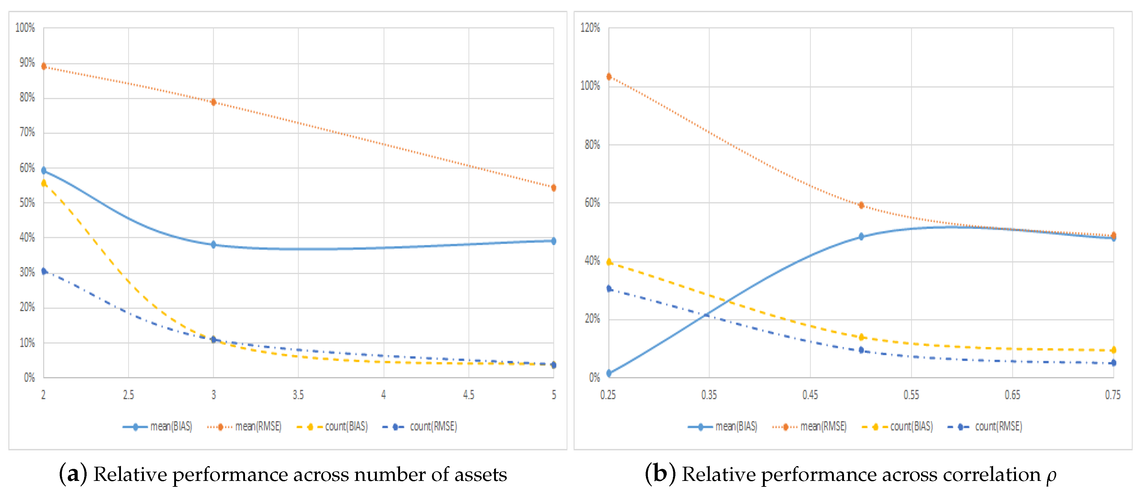
In the LSMC method, we again consider the complete set of polynomials of order $L=3$ or less and therefore use a total of 10, 20 and 56 regressors when the dimension of the problem, M, is 2, 3 and 5, respectively. In all cases, we use $I=100$ independent simulations with $N=$ 100,000 simulated paths. We consider options with different features and different asset dynamics. In particular, we consider three values of the strike price, $K=[95,100,105]$, the time to maturity, $T=[0.5,1,2]$ years, the volatility, $\sigma =[10\%,20\%,40\%]$, the correlation between the assets, $\rho =[0.25,0.50,0.75]$, and the number of assets, $M=[2,3,5]$, for a total of $3^5=243$ options. Pricing options in multiple dimensions quickly become computationally complex, and for this reason, we consider a smaller sample of options than in the benchmark case. Overall, our results show that the average RMSE obtained with the symmetric method is $36\%$ smaller than that obtained with the regular method, and the RMSE is smallest for $87\%$ of the individual options when using the symmetric method. These results clearly show that symmetry is valuable also for more advanced multivariate models.

Figure 5a and Panel A of

Table 6. Pricing errors across model characteristics in a multivariate model.

Panel A: Across Number of Assets M
	Absolute Metrics				Counting Metrics
	Regular Call		Symmetric Call		Regular Call		Symmetric Call
$\mathit{M}$	Bias	RMSE	Bias	RMSE	Bias	RMSE	Bias	RMSE
2	0.0021	0.0054	0.0012	0.0048	0.6420	0.7654	0.3580	0.2346
3	0.0099	0.0123	0.0038	0.0097	0.9012	0.9012	0.0988	0.0988
5	0.0319	0.0329	0.0125	0.0180	0.9630	0.9630	0.0370	0.0370
Panel B: Across Correlation $\mathit{\rho }$
	Absolute Metrics				Counting Metrics
	Regular Call		Symmetric Call		Regular Call		Symmetric Call
$\mathit{\rho }$	Bias	RMSE	Bias	RMSE	Bias	RMSE	Bias	RMSE
0.25	0.0073	0.0111	−0.0001	0.0115	0.7160	0.7654	0.2840	0.2346
0.5	0.0143	0.0161	0.0069	0.0096	0.8765	0.9136	0.1235	0.0864
0.75	0.0223	0.0234	0.0107	0.0114	0.9136	0.9506	0.0864	0.0494

This table shows pricing errors for the regular and symmetric method in a multivariate model for various values of the number of stocks M and correlation $\rho$. Results are based on $I=100$ independent simulations with $N=$ 100,000 paths. In each panel, we report results for the bias and RMSE in terms of the average metrics and counting metrics, i.e., the fraction of times a given method has the highest error metric.

show the results across the number of assets, M, and demonstrate clearly that our suggestion of pricing call options as put options becomes more important as the dimension, and hence the computational complexity, of the option increases. In particular, the relative error of the symmetric method in terms of RMSE in Figure 5a goes from $0.890$–$0.545$ as the dimension increases from 2–5. Moreover, when the dimension of the problem is high, the symmetric method almost always, in $96.3\%$ of the cases, has the lowest RMSE, as shown in Panel A of Table 6.

Figure 5b and Panel B of Table 6 show the results across the correlation between the assets, $\rho$. From the figure, it is seen that symmetry becomes more important when correlations between assets increase. In particular, in terms of the absolute metrics, the regular method performs on par with the symmetric method when the correlation is low and $\rho =0.25$, but when the correlation is high and $\rho =0.75$, the error in pricing of the symmetric method is only around half that of the regular method, as shown in Figure 5b. Moreover, the symmetric method is always the method that yields the smallest errors for the largest fraction of the options. For example, when correlations are high among the underlying assets, the symmetric method has larger RMSE for only $4.94\%$ of the options as shown in Panel B of Table 6.

The SV model of Heston (1993) is one of the most famous extensions to the constant volatility model. While it may not have been the first SV model, e.g., earlier examples include Hull and White (1987), Scott (1987) and Wiggins (1987), this particular model has emerged as the most important one and now serves as a benchmark against which many other SV models are compared. In the model of Heston (1993), the variance followed a Cox et al. (1985) process specified as:

$$d{v}_t=\kappa (\theta -v_t)dt+\sigma \sqrt{v_t}d{W}_{2,t}^Q.$$

(9)

Here, $\kappa$ represents the mean reversion rate of the variance, $\theta$ is the long-term variance, $\sigma$ is the volatility of volatility (vol of vol) and the stock dynamics and variance are allowed to be correlated with correlation coefficient $\rho$. Put-call symmetry also holds in this model as demonstrated by, e.g., Battauz et al. (2014), which also listed the appropriate changes of parameters. In particular, the paper shows that in the model of Heston (1993), the following parity holds between a call option and a put option:

$$C(S,r,q,K,V_0,\theta ,\kappa ,\sigma ,\rho )=P(K,q,r,S,V_0,\kappa \theta /(\kappa -\sigma \rho ),\kappa -\sigma \rho ,\sigma ,-\rho ).$$

(10)

In other words, a call option can be priced as a put option in which the stock price and the strike price and the interest rate and the dividend yield are interchanged, as was the case in the constant volatility setting, and in which the mean reversion, ${\kappa }^{\prime }$, the long-term variance, ${\theta }^{\prime }$, and the correlation, ${\rho }^{\prime }$, for the symmetric put option are changed to:

$${\kappa }^{\prime }=\kappa -\sigma \rho ,{\theta }^{\prime }=\theta \kappa /{\kappa }^{\prime },\mathrm{and}{\rho }^{\prime }=-\rho ,$$

(11)

where $\kappa$, $\theta$ and $\rho$ are the actual mean reversion, long-term variance and correlation.

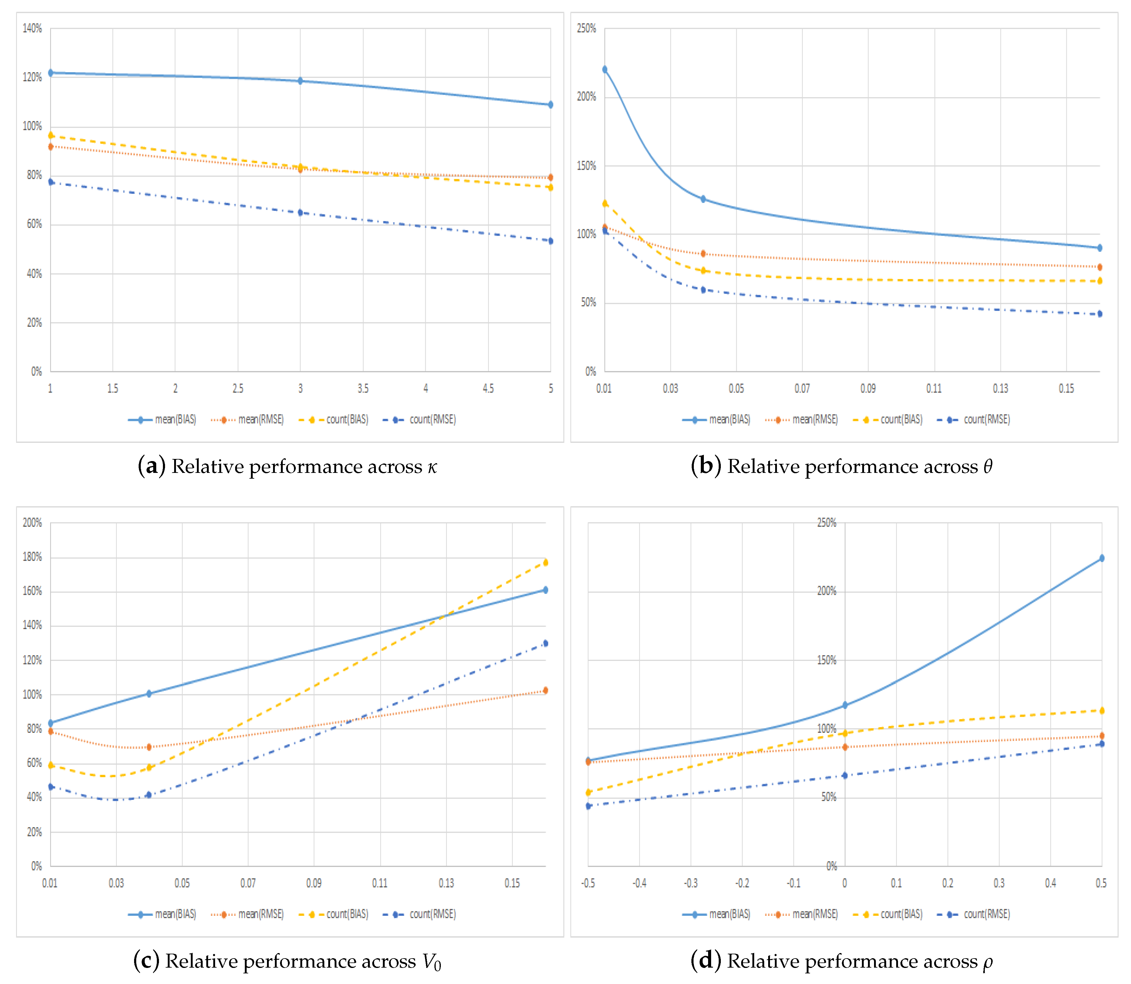
We again price each of the individual options $I=100$-times with independently-simulated state variables used in the LSMC method, which we implemented using $N=$ 100,000 paths. In the cross-sectional regressions, we use the complete set of polynomials in two dimensions of order $L=3$ or less as regressors for a total of 10 regressors including the constant term. We consider three different values of the strike price, $K=[90,100,110]$, the time to maturity, $T=[0.5,1,2]$ years, the mean reversion rate, $\kappa =[1,3,5]$, the long-term variance, $\theta =[0.01,0.04,0.16]$, the initial level of the variance, $V_0=[0.01,0.04,0.16]$, the volatility of volatility, $\sigma =[0.05,0.1,0.2]$, and the correlation between the two Brownian motions, $\rho =[-0.5,0,0.5]$, for a total of $3^7=2187$ options. Overall, our results show that the average RMSE obtained with the symmetric method is $14\%$ smaller than that obtained with the regular method, and the RMSE is smallest for $61\%$ of the individual options when using the symmetric method. These results clearly show that symmetry is valuable also for more advanced models, and though the results are somewhat closer to each other than with our benchmark model, this is to be expected since we are considering options here that have on average shorter maturities.

Figure 6 and

Table 7. Pricing errors across model characteristics in a stochastic volatility model.

Panel A: Across Mean Reversion $\mathit{\kappa }$
	Absolute Metrics				Counting Metrics
	Regular Call		Symmetric Call		Regular Call		Symmetric Call
$\mathit{\kappa }$	Bias	RMSE	Bias	RMSE	Bias	RMSE	Bias	RMSE
1	0.0084	0.0139	0.0102	0.0128	0.5089	0.5638	0.4911	0.4362
3	0.0055	0.0099	0.0066	0.0082	0.5446	0.6063	0.4554	0.3937
5	0.0053	0.0093	0.0058	0.0074	0.5706	0.6516	0.4294	0.3484
Panel B: Across Long-Term Variance $\mathit{\theta }$
	Absolute Metrics				Counting Metrics
	Regular Call		Symmetric Call		Regular Call		Symmetric Call
$\mathit{\theta }$	Bias	RMSE	Bias	RMSE	Bias	RMSE	Bias	RMSE
0.01	0.0028	0.0077	0.0061	0.0081	0.4486	0.4938	0.5514	0.5062
0.04	0.0045	0.0084	0.0057	0.0072	0.5748	0.6241	0.4252	0.3759
0.16	0.0119	0.0170	0.0108	0.0130	0.6008	0.7037	0.3992	0.2963
Panel C: Across Initial Variance ${\mathit{V}}_{\mathbf{0}}$
	Absolute Metrics				Counting Metrics
	Regular Call		Symmetric Call		Regular Call		Symmetric Call
${\mathit{V}}_{\mathbf{0}}$	Bias	RMSE	Bias	RMSE	Bias	RMSE	Bias	RMSE
0.01	0.0081	0.0115	0.0068	0.0090	0.6296	0.6818	0.3704	0.3182
0.04	0.0035	0.0088	0.0035	0.0062	0.6337	0.7051	0.3663	0.2949
0.16	0.0076	0.0128	0.0122	0.0131	0.3608	0.4348	0.6392	0.5652
Panel D: Across Correlation $\mathit{\rho }$
	Absolute Metrics				Counting Metrics
	Regular Call		Symmetric Call		Regular Call		Symmetric Call
$\mathit{\rho }$	Bias	RMSE	Bias	RMSE	Bias	RMSE	Bias	RMSE
−0.5	0.0096	0.0120	0.0074	0.0092	0.6488	0.6927	0.3512	0.3073
0	0.0060	0.0105	0.0070	0.0092	0.5075	0.6008	0.4925	0.3992
0.5	0.0036	0.0105	0.0081	0.0100	0.4678	0.5281	0.5322	0.4719

This table shows pricing errors for the regular and symmetric method in a stochastic volatility model for various values of the mean reversion rate, $\kappa$, long-term variance, $\theta$, initial volatility, $V_0$, and correlation, $\rho$. Results are based on $I=100$ independent simulations with $N=$ 100,000 paths. In each panel, we report results for the bias and RMSE in terms of the average metrics and counting metrics, i.e., the fraction of times a given method has the highest error metric.

show the results across the various values of the mean reversion rate, $\kappa$, the long-term variance, $\theta$, the initial level of the variance, $V_0$, and the correlation, $\rho$. The first thing to notice from the table is that across all these interesting parameters and parameter values, the symmetric method most of the time outperforms the regular approach. The two exceptions to this are options with very low long-term variance and $\theta =0.01$ and when the initial level of the variance is very high and $V_0=0.16$, where the RMSE is slightly lower with the regular method than with the symmetric method. In both of these cases, the symmetric method also has larger RMSE for more options than does the regular method, whereas in all the other cases, the symmetric method most often has the smallest RMSE.

In terms of performance across parameters, Figure 6 and Table 7 show that the symmetric method performs relatively better the faster the volatility mean reverts, i.e., the larger the value of $\kappa$ in Figure 6a, and the larger the value of the long-term variance, i.e., the larger the value of $\theta$ in Figure 6b. The last of these findings is completely in line with the results from our benchmark model where symmetric pricing was most important for high values of the asset volatility. Figure 6d shows that the symmetric method performs relatively better when correlations are negative, which is indeed the empirically most relevant case in the stochastic volatility model of Heston (1993). When the correlation is highly negative and $\rho =-0.5$, the symmetric method has errors in terms of bias and RMSE that are around $25\%$ lower than the regular method and has the largest errors for only around one third of the individual options. The effect on the relative performance of the initial variance, $V_0$, is less clear cut though Figure 6c does indicate that the symmetric method performs relatively better when $V_0$ is not too extreme, and in particular not too high.

6. Discussion

The fact that pricing call options using the symmetry method works best for most and along some dimensions almost all of the options considered is great news. However, since it does not perform the best for all the options, it leaves the obvious question of when to choose one method over the other. As it is, the only solid recommendations that arise from Section 4 and Section 5 are that using the symmetric method with standard choices of the number of paths and number of regressors used in the LSMC method is relatively better the longer the maturity and the larger the volatility and that the methods become more similar when simulating a very large number of paths, e.g., when N is as large as 500,000, and that they diverge when using a large number of regressors, e.g., when L is as large as 15. In this section, we first examine the performance of the individual methods in terms of a relative efficiency measure, which compares the performance of a method to what could have been obtained optimally. Then, using properties of the out-of-sample method for pricing, we propose a method for selecting which specification to use across the methods and the number of regressors, which is simple to implement and achieves a very high degree of efficiency.

6.1. Efficiency as an Alternative Metric

Until know, we have compared performance metrics, i.e., the RMSE or the number of times a method works the best or worst, for the regular and symmetric pricing methods, respectively. An alternative and perhaps more interesting metric for “practitioners” is what one stands to lose in terms of increased pricing errors by picking and sticking to one particular method instead of using the optimal method for a given individual option in our sample. To examine this, we now consider a metric, which we will refer to as the “efficiency” given by the ratio of a specific method’s RMSE to the optimal and infeasible RMSE that could be obtained if one knew which method to use for each of the individual options.

Table 8. Efficiency across the number of paths N and regressors L.

Panel A: Results across Number of Paths N
	RMSE			Efficiency		Count
$\mathit{N}$	Call	SCall	Optimal	Call	SCall	Call	SCall
20,000	0.0426	0.0178	0.0166	38.91%	92.98%	30.85%	69.15%
50,000	0.0480	0.0131	0.0125	26.00%	95.56%	20.00%	80.00%
100,000	0.0602	0.0104	0.0102	16.99%	98.33%	11.81%	88.19%
200,000	0.0540	0.0100	0.0100	18.49%	99.95%	2.34%	97.66%
500,000	0.0556	0.0124	0.0123	22.04%	98.83%	11.65%	88.35%
Panel B: Results across Number of Regressors $\mathit{L}$
	RMSE			Efficiency		Count
$\mathit{L}$	Call	SCall	Optimal	Call	SCall	Call	SCall
2	0.0832	0.0351	0.0345	41.41%	98.17%	10.14%	89.86%
3	0.0602	0.0104	0.0102	16.99%	98.33%	11.81%	88.19%
5	0.0201	0.0117	0.0099	49.34%	84.48%	60.99%	39.01%
9	0.0328	0.0154	0.0150	45.78%	97.21%	28.77%	71.23%
15	0.0625	0.0187	0.0184	29.39%	98.00%	24.45%	75.55%

This table shows the efficiency across the number of paths, N, and regressors, L. Efficiency is measured as the optimal RMSE, conditional on knowing which of the two methods yields the lowest RMSE, as a fraction of the RMSE of the regular or symmetric method, respectively. Panel A reports results for different values of the number of simulated paths, N, and Panel B reports results for different values of the number of regressors, L. In addition to the efficiency, the table also reports the fraction of times for which the regular and symmetric method provide the lowest RMSE, respectively.

shows the efficiency of the two methods using in-sample pricing for various values of N and L in Columns 5 and 6. For comparison, the fraction of the options for which a particular model performs the best in terms of having the lowest RMSE is also reported in Columns 7 and 8.13 Panel A of Table 8 clearly shows that the symmetric method performs extremely well across the number of simulated paths, and one would never lose more than $7\%$ from using this method. In fact, for most realistic specifications, i.e., when $N\ge$ 100,000, the loss is less than $2\%$. The regular method, on the other hand, often has an efficiency of just around $20\%$, meaning that if this method was used to price the sample of options, one would lose around $80\%$ compared to what could optimally be obtained.

Panel B of the table is, given the results in the previous section on robustness, even more interesting. In particular, the previous results showed that for some specification, i.e., when picking $L=5$, the symmetric method actually has larger RMSE than the regular method for most options. The row labelled $L=5$ in Table 8, however, shows that even in this case where the symmetric RMSE is the lowest for only $39\%$ of the options, the method’s efficiency is above $84\%$. That is, even for settings when the regular method is the best, measured by minimizing the RMSE, for $61\%$ of the options when using the symmetric method, you would not lose more than $16\%$ compared to what could be optimally obtained had you known what would be the best method to use for the individual options. It is also striking that if you, on the other hand, would use the regular method for all options, the efficiency is only around $49\%$ in spite of the fact that this is the method that has the lowest RMSE for most of the options.

Table 9. Efficiency across number of paths N and regressors L using OSpricing.

Panel A: Results across Number of Paths N
	RMSE			Efficiency		Count
$\mathit{N}$	Call	SCall	Optimal	Call	SCall	Call	SCall
20,000	0.1303	0.0163	0.0163	12.54%	100.00%	0.03%	99.97%
50,000	0.0986	0.0166	0.0166	16.81%	100.00%	0.22%	99.78%
100,000	0.0851	0.0157	0.0156	18.38%	99.86%	5.28%	94.72%
200,000	0.0590	0.0190	0.0185	31.36%	97.52%	21.22%	78.78%
500,000	0.0708	0.0106	0.0106	14.93%	99.99%	0.58%	99.42%
Panel B: Results across Number of Regressors $\mathit{L}$
	RMSE			Efficiency		Count
$\mathit{L}$	Call	SCall	Optimal	Call	SCall	Call	SCall
2	0.0983	0.0438	0.0437	44.42%	99.63%	6.78%	93.22%
3	0.0851	0.0157	0.0156	18.38%	99.86%	5.28%	94.72%
5	0.0498	0.0079	0.0079	15.79%	99.03%	7.97%	92.03%
9	0.0427	0.0091	0.0090	21.01%	98.49%	11.10%	88.90%
15	0.0458	0.0117	0.0116	25.36%	99.36%	7.90%	92.10%

This table shows the efficiency across the number of paths, N, and regressors, L, using out-of-sample pricing. Efficiency is measured as the optimal RMSE, conditional on knowing which of the two methods yields the lowest RMSE, as a fraction of the RMSE of the regular or symmetric method, respectively. Panel A reports results for different values of the number of simulated paths, N, and Panel B reports results for different values of the number of regressors, L. In addition to the efficiency, we also report the fraction of times for which the regular and symmetric method provide the lowest RMSE, respectively.

shows the efficiency of the two methods using out-of-sample pricing for various values of N and L in Columns 5 and 6. The first thing to notice form this table is that when using out-of-sample pricing, i.e., when a new set of paths is used for pricing, the efficiency of the symmetric method is extremely high, and often above $99\%$, across both the choice of the number of paths, N, and the number of regressors, L. Compared to the in-sample results in Table 8, the efficiency of the symmetric method is most of the time improved, the exception being when using $N=$ 200,000 paths in the simulation. For the regular method, on the other hand, efficiency is generally much lower, as low as $15\%$, and does not improve in any systematic way when using out-of-sample pricing. In conclusion, although the symmetric method is not always the model that has the smallest RMSE, the efficiency of this method is generally very high, always significantly higher than that of the corresponding regular method, and therefore, the costs of using this method are always reasonably low. Our suggestion is therefore very naturally to use the symmetric method for call option pricing.

6.2. Picking the Best Configuration

Although we recommend to always use the symmetric method for call option pricing, you may still wonder if it is possible to improve on this recommendation, i.e., if it is possible to pick the “right” model using some “observables”. This is essentially a question of classification. A straightforward classification variable is the estimated price. In particular, we know that when using the out-of-sample pricing technique, estimates are in expectation low biased. Moreover, while we expect the estimates to increase when increasing the number of regressors, L, initially, as this improves the polynomial approximation, when L becomes very large and over fitting to the paths used to determine the optimal exercise strategy becomes a problem, the estimated out-of-sample price could decrease. When comparing results for several different values of L and different methods, i.e., regular versus symmetric, one could therefore propose to choose the method that maximizes the out-of-sample price. In particular, this should result in picking the method that has the smallest bias, and this would potentially also be the method with a small RMSE. The results from implementing this classification strategy are shown in

Table 10. Efficiency across the number of regressors L using OS pricing.

Panel A: Results for Individual Values of L
	RMSE			Classified			Local Efficiency		Global Efficiency
L	Call	SCall	Optimal	RMSE	Picked	Efficiency	Call	SCall	Call	SCall
2	0.0983	0.0438	0.0437	0.0437	93.34%	99.83%	44.42%	99.63%	7.45%	16.72%
3	0.0851	0.0157	0.0156	0.0157	95.36%	99.65%	18.38%	99.86%	8.61%	46.79%
5	0.0498	0.0079	0.0079	0.0079	95.74%	99.66%	15.79%	99.03%	14.72%	92.27%
7	0.0440	0.0082	0.0081	0.0081	96.77%	99.78%	18.36%	98.31%	16.65%	89.17%
9	0.0427	0.0091	0.0090	0.0090	97.44%	99.90%	21.01%	98.49%	17.15%	80.41%
11	0.0430	0.0100	0.0099	0.0099	97.89%	99.96%	22.92%	98.85%	17.02%	73.40%
15	0.0458	0.0117	0.0116	0.0116	99.17%	99.99%	25.36%	99.36%	16.01%	62.75%
Panel B: Results for Multiple Values of $\mathit{L}$
	RMSE			Classified			Local Efficiency		Global Efficiency
$\mathit{L}$	Call	SCall	Optimal	RMSE	Picked	Efficiency	Call	SCall	Call	SCall
All	0.0379	0.0074	0.0073	0.0074	90.43%	98.98%	99.99%	99.99%	19.33%	98.36%

This table shows the relative efficiency of the two methods using out-of-sample pricing across the number of regressors, L. Efficiency is measured as the optimal RMSE, conditional on knowing which of the methods yields the lowest RMSE for a given individual option in our large sample of 3125 options, as a fraction of the RMSE of the regular and symmetric method, respectively. Panel A report results for different values of the number of regressors used in the cross-section regression, L, and Panel B reports results across all the values of L in Panel A. The result in the column headed “Optimal” corresponds to selecting the method with the minimum RMSE either for a given L, in Panel A, or across all values of L, in Panel B. The results in the column headed “Classified” correspond to what would be obtained if the method with the highest price is used, either for a given L or across all values of L and reports the resulting RMSE, the fraction of options for which the method with the lowest RMSE was actually picked and the efficiency of this method compared to the corresponding optimal method. In Panel A, “Local Efficiency” is measured relative to the optimal RMSE for a given value of L. In Panel B, “Local Efficiency” is measured relative to the minimum RMSE obtained for the regular and symmetric method, respectively, across all values of L. In both panels, results in the column headed “Global Efficiency” report the efficiency of the two methods compared to the best possible RMSE of $0.0073$ reported in Panel B.

.

Panel A in Table 10 reports results for individual values of L, i.e., when the method, regular or symmetric, that has the highest price for a given value of L is picked. The first thing to notice from this panel is that the right method for a given option is picked at least $93\%$ of the time, and the efficiency of this method is always above $99\%$. The symmetric method clearly performs the best on average for all values of L, and this method does have a very high “local” efficiency, that is compared to the optimal RMSE for a particular value of L. The regular method, on the other hand, has a much lower efficiency. Compared to the efficiency of the individual methods, the panel shows that classification according to maximum price does improve on the RMSE in all but one case. In terms of “global” efficiency though, the performance of the methods varies greatly across L.

Panel B in Table 10 reports results across all the values of L used in Panel A, i.e., in this panel, the optimal RMSE is picked across both methods and the values of L. The first thing to notice from this panel is that the classification method performs very well and picks the right method more than $90\%$ of the time and has a very high efficiency of close to $99\%$. Picking the symmetric method that has the highest price across L also results in estimates that are very efficient, although the optimal RMSE is slightly lower. The efficiency of the regular method is below $20\%$ when compared to the globally optimal method, although measured locally across L picking the method with the highest price results in estimates with an RMSE very close to the minimum RMSE for this method.

The results above show that when using out-of-sample pricing, it is possible to derive a simple classification algorithm that achieves very high efficiency. In reality, the algorithm ends up picking the symmetric method most of the time, and if you only pick within this method, the loss in efficiency is very small, i.e., it decreases from $98.98$–$98.36\%$. Thus, it is possible to save on the computational time by only considering this method. Moreover, for most of the options, the highest price is achieved with $L=5$ when using the symmetric method, and if, instead of picking among all the possible values of L in the table, you only consider $L\le 7$, the global efficiency decreases only marginally to $98.24\%$.14 This approach thus yields very good estimates across our large sample of options, and it is easy to implement. It is not possible to come up with a similar approach when using in-sample pricing though.

7. Conclusions

This paper shows that it is possible to improve significantly on the estimated call prices obtained with a state-of-the-art algorithm, the Least Squares Monte Carlo (LSMC) method of Longstaff and Schwartz (2001), for option pricing using regression and Monte Carlo simulation by using Put-Call Symmetry (PCS). PCS holds widely and in the classical Black–Scholes–Merton case, for example, implies that a call option has the same price as an otherwise similar put option where strike price and stock level and where interest rate and dividend yield are interchanged, respectively. The immediate implication is that path-wise payoffs in simulations are bounded above by the strike price instead of being unbounded, and for methods that use regression to determine the optimal early exercise strategy, this leads to much improved estimates of the stopping time and more precise option price estimates as measured by, for example, the Root Mean Squared Error (RMSE). Our results show that, for a large sample of options with characteristics of relevance in real-life applications, the symmetric method on average performs much better than the regular pricing method, is the best method for most of the options, never performs very poorly and as a result is very efficient compared to an optimal, but unfeasible method that picks the method with the smallest RMSE. When using out-of-sample pricing, a simple classification algorithm is proposed that, by optimally selecting among estimates from the symmetric method with a reasonably small order used in the polynomial approximation, achieves a relative efficiency of more than $98\%$ compared to the infeasible, but optimal method that minimizes the RMSE across all estimates. Our results also show that the relative importance of using the symmetric method increases with option maturity and with asset volatility and using symmetry methods to price long-term options in high volatility situations improves massively on the price estimates. The LSMC method is routinely used to price real options, many of which are call options with long maturity on volatile assets, for example energy. We therefore conjecture that pricing such options using the symmetric method could improve the estimates significantly by decreasing their bias and RMSE by orders of magnitude.

References

- Battauz, Anna, Marzia De Donno, and Alessandro Sbuelz. 2014. The Put-Call Symmetry for American Options in the Heston Stochastic Volatility Model. Mathematical Finance Letters 7: 1–8. [Google Scholar]
- Boyle, Phelim P., and Yiu Kuen Tse. 1990. An Algorithm for Computing Values of Options on the Maximum or Minimum of Several Assets. Journal of Financial and Quantitative Analysis 25: 215–27. [Google Scholar] [CrossRef]
- Chow, Yuan-Shih, Herbert Robbins, and David Siegmund. 1971. Great Expectations: The Theory of Optimal Stopping. New York: Houghton Mifflin. [Google Scholar]
- Cox, John C., Jonathan E. Ingersoll, and Stephen A. Ross. 1985. A Theory of the Term Structure of Interest Rates. Econometrica 53: 385–408. [Google Scholar] [CrossRef]
- Cox, John C., Stephen A. Ross, and Mark Rubinstein. 1979. Option pricing: A simplified approach. Journal of Financial Economics 7: 229–63. [Google Scholar] [CrossRef]
- Detemple, Jerome. 2001. American Options: Symmetry Properties. In Handbooks in Mathematical Finance: Topics in Option Pricing, Interest Rates and Risk Management. Edited by Elyes Jouini, Jaksa Cvitanic and Marek Musiela. Cambridge: Cambridge University Press, pp. 67–104. [Google Scholar]
- Duffie, Darrell. 1996. Dynamic Asset Pricing Theory. Princeton: Princeton University Press. [Google Scholar]
- Grabbe, J. Orlin. 1983. The Pricing of Call and Put Options of Foreign Exchange. Journal of International Money and Finance 2: 239–53. [Google Scholar] [CrossRef]
- Heston, Steven L. 1993. A Closed-Form Solution for Options with Stochastic Volatility with Applications to Bond and Currency Options. Review of Financial Studies 6: 327–43. [Google Scholar] [CrossRef]
- Hull, John, and Alan White. 1987. The Pricing of Options on Assets with Stochastic Volatilities. Journal of Finance 42: 281–300. [Google Scholar] [CrossRef] [Green Version]
- Karatzas, Ioannis. 1988. On the Pricing of American Options. Applied Mathematics and Optimization 17: 37–60. [Google Scholar] [CrossRef]
- Longstaff, Francis A., and Eduardo S. Schwartz. 2001. Valuing American Options by Simulation: A Simple Least-Squares Approach. Review of Financial Studies 14: 113–47. [Google Scholar] [CrossRef]
- McDonald, Robert C., and Mark Schroder. 1998. A Parity Result for American Options. Journal of Computational Finance 1: 5–13. [Google Scholar] [CrossRef]
- Royden, Halsey. 1988. Real Analysis. Upper Saddle River: Prentice Hall, Inc. [Google Scholar]
- Schroder, Mark. 1999. Changes of Numeraire for Pricing Futures, Forwards, and Options. Review of Financial Studies 12: 1143–63. [Google Scholar] [CrossRef]
- Scott, Louis O. 1987. Option Pricing When the Variance Changes Radomly: Theory, Estimation, and an Application. Journal of Financial and Quantitative Analysis 22: 419–38. [Google Scholar] [CrossRef]
- Stentoft, Lars. 2004a. Assessing the Least Squares Monte-Carlo Approach to American Option Valuation. Review of Derivatives Research 7: 129–68. [Google Scholar] [CrossRef]
- Stentoft, Lars. 2004b. Convergence of the Least Squares Monte Carlo Approach to American Option Valuation. Management Science 50: 1193–203. [Google Scholar] [CrossRef]
- Wiggins, James B. 1987. Option Values Under Stochastic Volatility: Theory and Empirical Estimates. Journal of Financial Economics 19: 351–72. [Google Scholar] [CrossRef]