Article

News Co-Occurrences, Stock Return Correlations, and Portfolio Construction Implications

1
Gabelli School of Business, Fordham University, New York, NY 10023, USA
2
Chatham High School, Chatham, NJ 07928, USA
*
Author to whom correspondence should be addressed.
J. Risk Financial Manag. 2019, 12(1), 45; https://doi.org/10.3390/jrfm12010045
Submission received: 22 February 2019 / Revised: 12 March 2019 / Accepted: 14 March 2019 / Published: 19 March 2019
(This article belongs to the Special Issue Empirical Asset Pricing)

Abstract

:
In this paper, we construct a sample of news co-occurrences using big data technologies. We show that stocks that co-occur in news articles are less risky, bigger, and more covered by financial analysts, and economically-connected stocks are mentioned more often in the same news articles. We decompose a news co-occurrence into an expected component and a shock component. We find that it is the shock component that arouses abnormal retail investor attention. The expected and shock components significantly predict return correlations 12 months into the future. Finally, a global minimum variance (GMV) portfolio with the covariance matrix augmented by the predictive power of news co-occurrences for future return correlations produces relatively superior performance compared to the benchmark GMV portfolio.

1. Introduction

Big data is rapidly changing the way financial markets work. Banks use big data analytics as a tool in credit risk management. Investment companies use big data processing and machine learning capabilities to process countless data points every day, helping them construct profitable stock portfolios. Insurance companies use big data in pricing, underwriting, and risk selection. Big data is also used extensively in academia. For example, researchers perform textual analysis to calculate the readability and sentiment of corporate disclosures1 and measure political uncertainty at the market level (see Baker et al. 2016).
In this paper, we explore a unique situation for corporate news coverage in which different firms co-occur in one news article. We construct a sample of news co-occurrences using big data technologies and link news co-occurrences to stock information. We explore the rich information embedded in news co-occurrences and attempt to answer several important and firmly-related questions. First, do news co-occurrences vary systematically across different firms? Second, how do attention-constrained investors respond to news co-occurrences? Third, do news co-occurrences explain contemporaneous and future stock return co-movements? Finally, can the explanatory ability of news co-occurrences for return co-movements improve portfolio construction?
We begin our empirical analyses by investigating the cross-sectional variation in news co-occurrences. Intuitively, economically-connected firms are more likely to be covered in the same news article. First, firms operating in the same sector are connected due to exposures to similar fundamental risks. Second, firms are connected through customer-supply relationships. For example, Apple is a major customer of Intel. It supplies about 5% of Intel’s annual revenue according to the supply chain analysis reported by Bloomberg. A slower adoption rate of Apple’s new iPhone can lead to lower stock prices for both Apple and Intel because the former may cut new iPhone production due to the weaker-than-expected demand. Last, past studies indicate that stock prices of firms located in the same area are affected by common area-specific risks. The work in Pirinsky and Wang (2006) documented co-movement among firms headquartered in the same location. The work in Korniotis and Kumar (2013) showed that local stock returns vary with local business cycles in a predictable manner. The work in Parsons et al. (2016) documented a positive lead-lag stock return relation between neighboring firms operating in different sectors.
Consistent with our conjectures, we show that stocks connected through operating in the same sector, having a supply-chain-based relationship, or having headquarters located in a neighboring area co-occur more often in news articles. According to our study, an extant economic linkage increases the number of news occurrences by 2–5% after controlling for everything else. We also find that stocks having similar characteristics such as less systematic risk, bigger size, and more analyst coverage tend to have more news co-occurrences, but these stock characteristics have much smaller explanatory power than the economic linkages.
We then study how news occurrences impact investor attention. In Kahneman (1973), the theory of attention indicates that attention is a scarce cognitive resource. Subsequently, a large body of psychological research shows that there is a limit to the central cognitive-processing capacity of the human brain.2 The implication of attention theory in financial markets is that limited availability of time and cognitive resources imposes constraints on how fast investors can process information. Theoretical models have shown that limited investor attention can lead to securities market underreaction to information and, thus, slow price adjustments (Hirshleifer and Teoh 2003; Peng 2005; Peng and Xiong 2006; Hirshleifer et al. 2009). These predictions have been confirmed by recent empirical findings that prices of securities underreact to value-relevant public information due to limited investor attention (see, e.g., Huberman and Regev 2001; Hirshleifer et al. 2004; 2009; 2013; Hou and Moskowitz 2005; Hong et al. 2007; DellaVigna and Pollett 2007, 2009; Cohen and Frazzini 2008; Bali et al. 2014). Since investors, retail investors in particular (see e.g., Ben-Rephael et al. 2017; Liu et al. 2018), have limited attention and processing power, stocks that attract attention are more likely to be purchased, while stocks that do not attract attention are often ignored. Consistent with this evidence, the work in Barber and Odean (2008) showed that retail investors, whose attention constraints are binding, are more likely to buy attention-grabbing stocks.
Recognizing that investor attention is a crucial condition for investors to take notice of news occurrences, we investigate how retail investors respond to news co-occurrences. We find that retail investors react positively to news occurrences. Moreover, it is the shock not the expected component of news co-occurrence that attracts more investor attention. One unit increase in unexpected news co-occurrences is associated with an increase of more than two standard deviations in abnormal retail investor attention.
Built on the evidence that news co-occurrences are significantly related to economic linkages and the shock components of news co-occurrences significantly impact retail investor attention, we argue that stock prices of firms that appear in the same news article are expected to move strongly together. First, stock prices of economically-connected firms tend to be highly correlated because they are exposed to similar fundamental risks. Second, attention-constrained investors are more likely to purchase stocks that attract their attention. Therefore, an unexpected news co-occurrence can lead investors to add the in-the-news stocks in their portfolios. We find that indeed news co-occurrences are positively associated with contemporaneous stock return correlations. The positive relation is much stronger for expected news co-occurrences than for unexpected news co-occurrences. A one-unit increase in expected news co-occurrence is related to an increase in contemporaneous return correlation by more than 0.05, which is economically significant given that the average return correlation of stocks in our sample is around 0.41.
Classic asset pricing theories are typically based on the assumption that markets are efficient in the sense that value-relevant public information is impounded into asset prices with lightning speed, so that stock prices are unpredictable. However, the finance literature has documented return anomalies in a variety of contexts that are hard to reconcile with the efficient market hypothesis (see Harvey et al. (2016) for a comprehensive list of these studies). In this paper, we focus on a different important question: Do news co-occurrences predict stock return correlations? We find strong evidence that more news co-occurrences significantly predict higher future return correlations even after accounting for persistence in return correlations. The predictive power of the expected component of news co-occurrences does not decay as the forecasting horizon increases. We further find that more unexpected news co-occurrences together with higher abnormal investor attention predict higher return correlations.
Last, we explore the implications of news co-occurrences for portfolio construction. In Markowitz’s (1952) paradigm, the objective of an investor is to choose a portfolio on the efficient frontier under the assumption that she/he has the perfect information on the model parameters: the expected returns on individual assets and the corresponding covariance matrix. In the real world, however, she/he has to estimate the parameters using historical data. Numerous studies have shown that bad estimates based on the historical approach that arise from estimation errors can render inferior performance ex-post.3 Since Merton (1980), many researchers have shifted their efforts to the global minimum variance (GMV) portfolio, whose weights depend solely on the more stable covariance matrix. For example, Jagannathan and Ma (2003) and DeMiguel et al. (2014) showed that the GMV portfolio outperforms portfolios that require estimating mean returns. Motivated by these findings, we explore the implications of news co-occurrences for constructing the GMV portfolio. We show that a GMV portfolio with the covariance matrix augmented by the predictive power of news co-occurrences for future return correlations produces smaller ex-post variance than the benchmark GMV portfolio.
Our study contributes to the literature in several ways. First, we quantify the effects of economic linkages on the frequency of news co-occurrence. Second, we show that in the context of news co-occurrence, it is not “in-the-news” per se, but the surprise component that attracts more investor attention. Third, we show that stock return co-movements increase with news co-occurrences, and such increased co-movements cannot be explained away by economic linkages, well-known stock characteristics, and after accounting for persistence in return correlations. Fourth, different from previous asset pricing studies that primarily analyze the lead-lag return relations between connected stocks, we focus on the predictability of news co-occurrence for future return correlations. Last, unlike past studies on portfolio construction that attempted to improve estimation of the covariance matrix using historical time-series data, we explore the rich information in the large cross-section of news co-occurrences and build the predictive power of news co-occurrences for future return correlations into the covariance matrix.
This paper is organized as follows. Section 2 describes the data and variables. Section 3 investigates how news co-occurrences vary systematically across different pairs of stocks. Section 4 examines how retail investors respond to news co-occurrences. Section 5 investigates the contemporaneous and predictive relations between news co-occurrences and stock return correlations. Section 6 explores the implications of news co-occurrences for portfolio construction. Section 7 concludes the paper.

2. Data and Variable Definitions

In this section, we discuss the data sources and define the variables used in the empirical analyses. Our sample includes the Standard & Poor’s 500 large-cap stocks, 400 mid-cap stocks, and 600 small-cap stocks (S&P 1500 stocks) covering the period from 2002–December 2016. Our news co-occurrence sample covers the period of May 2007–December 2016.4 We first explain how we construct the sample of news co-occurrences and then provide the definitions of the variables used in our study.

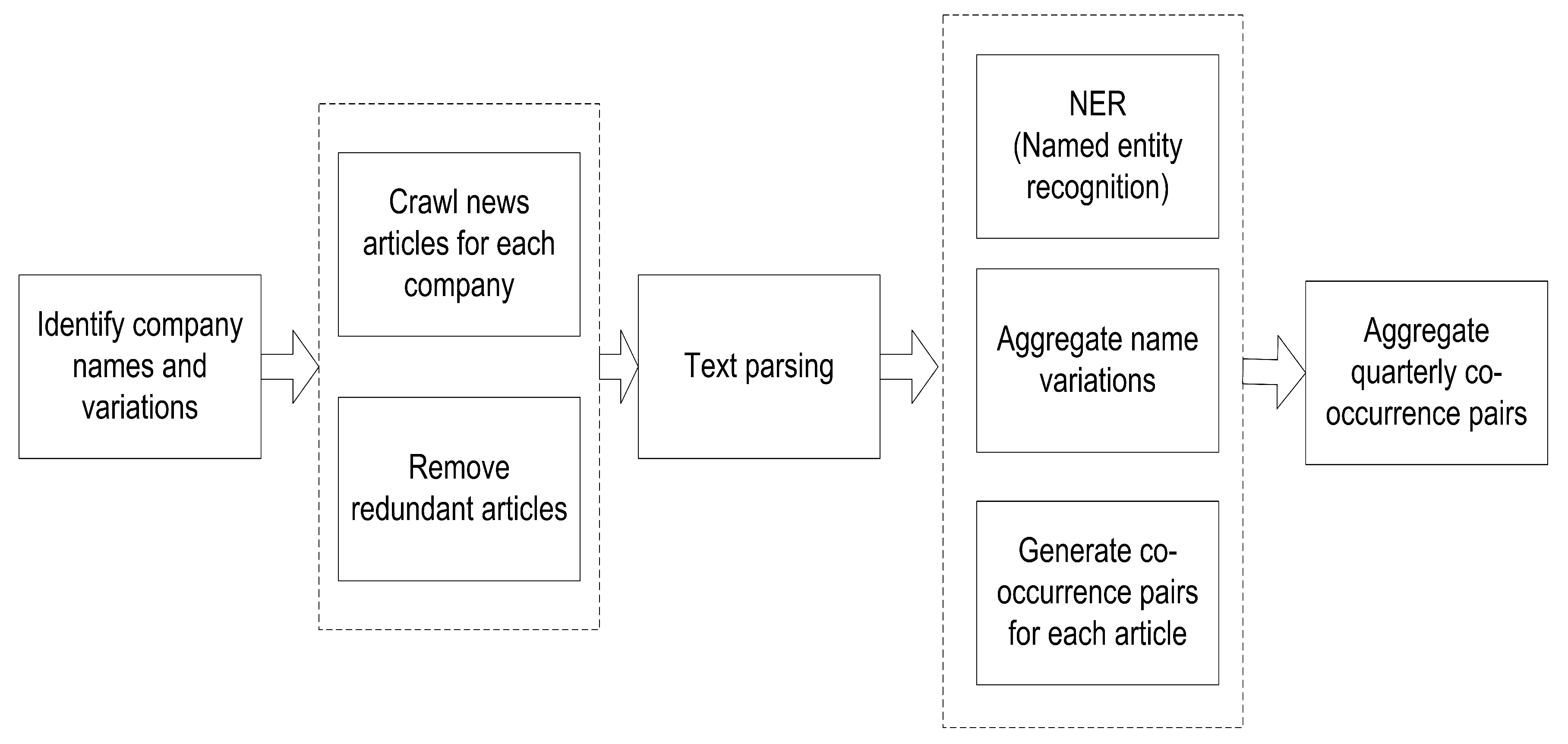
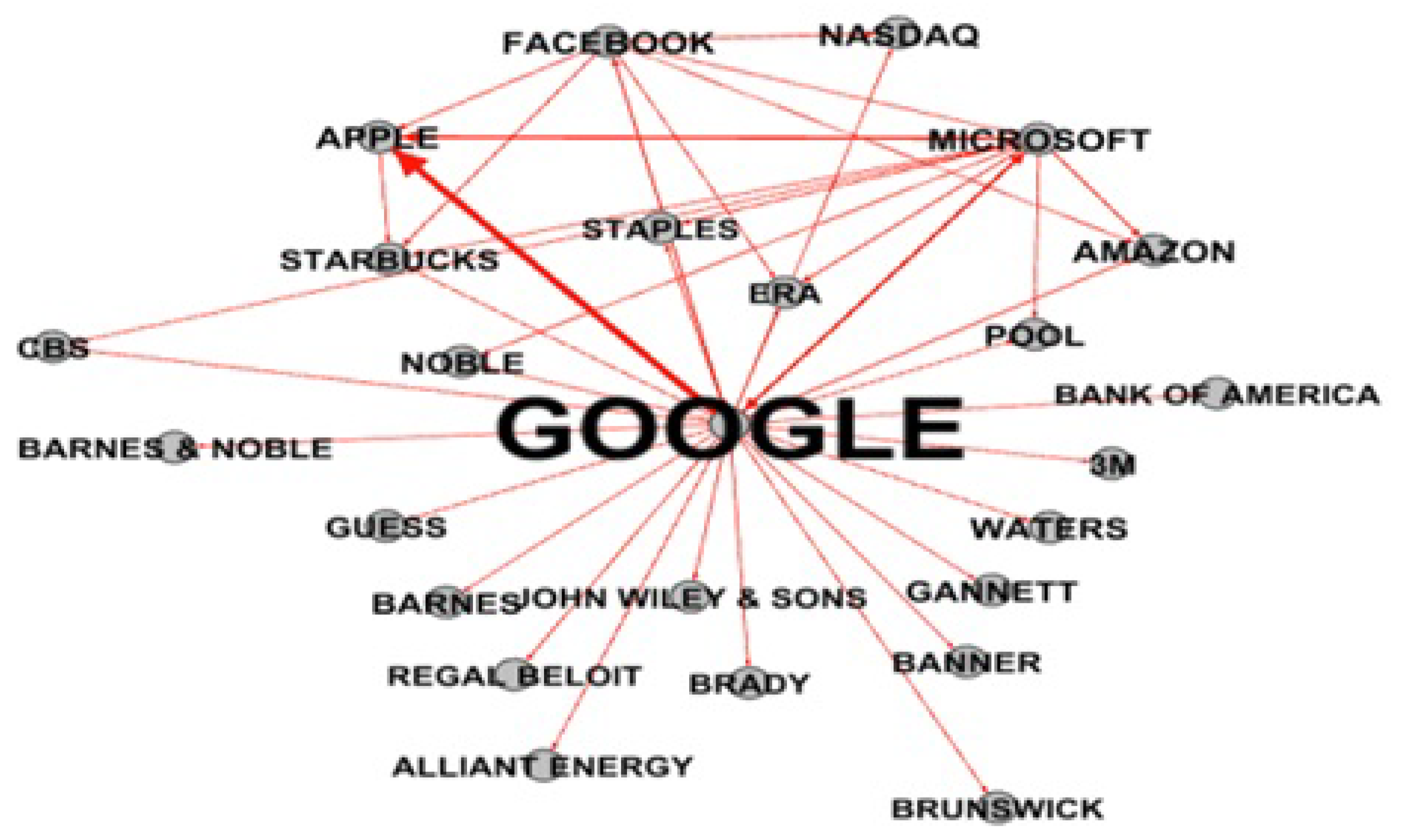
2.1. News Co-Occurrence Analysis

Text mining is a powerful analytics tool in leveraging information from news articles (Chen et al. 2012). It is capable of discovering hidden knowledge from a large volume of data. Text mining research deals with a variety of problems including text summarization, document and information retrieval, text categorization, authorship identification, and entity extraction and relation extraction (Witten et al. 2004). Previous studies have suggested the correlation between news articles and stock price (Schumaker and Chen 2009; Yu et al. 2013). However, they mostly relied on topics mining and sentiment analysis. For example, Schumaker and Chen (2009) extracted noun phrases from news articles to detect breaking news. This information is then combined with regression analysis to improve stock price prediction accuracy. The work in Yu et al. (2013) and Schumaker et al. (2012) both extracted sentiment in news articles to correlate with stock price. Co-occurrence analysis is often used to identify company relations from news articles. For example, the work in Ma et al. (2011) built an inter-firm network from firm name co-occurrence citations in news and inferred competitor relationships from network properties. The work in Bao et al. (2008) identified and ranked competitors based on the results returned from search engine co-occurrence. However, the correlation between co-occurrence and stock price return is not studied in information systems research.
Figure 1 illustrates our process of deriving co-occurrence information in news articles. We first identify company names from the S&P 1500 list. Lexis-Nexis is used as our data source for news articles.5 An automatic crawling algorithm searches news articles that contain each company name within each year. Because the same news article may be returned from different searches, we removed redundant articles by checking the title, date, and author of the article. A total of 2,671,004 news articles that covered years 2007–2016 were retained after the crawling process. These articles covered a total of 1434 companies. The missing companies were those not generating results from the news search.
These news articles were processed to extract meta information such as publish time, source, author, title, and news text. We ran the Stanford Named Entity Recognizer (NER) program to extract named entities.6 NER aims to extract and classify rigid designators (Nadeau and Sekine 2007). There are many types of named entities in text such as company name, person name, and product name. These named entities are then mapped against our company name list and their variations. Performing NER before mapping company names is necessary to handle generic keywords that appear in company names. For example, Gap Inc is sometimes referred to as Gap. If we map the keyword “Gap” directly, we may mistakenly count the generic keyword “gap” as the occurrence of the company name. We also manually created a name variation table to increase the coverage of our mapping algorithm. A company’s name can appear in multiple forms, a problem referred to as name variation. Since we are only interested in the S&P 1500 company names, a name variation table was the easiest way to address the problem. For example, Walmart Inc can appear as Wal Mart, Walmart, and Wal-Mart Stores, Inc. The appearance of these names was aggregated to Walmart Inc. We then identified if a news article had multiple company names. If more then two names were mentioned in one news article, we considered all of them to be pairs of co-occurrence.
Finally, these co-occurrence pairs were aggregated monthly. Figure 2 illustrates co-occurrence pairs extracted from news articles in 2012, fourth quarter. The thickness of links indicates the frequency of co-occurrence.

2.2. Stock Characteristics

The daily and monthly return data and the standard industry classification (SIC) code were acquired from the Center for Research in Security Prices (CRSP). We adjusted stock returns for delisting in order to avoid survivorship bias (Shumway 1997).7 Accounting data and zip codes of firms’ headquarters were obtained from the Compustat database. Analyst coverage data came from the the Institutional Brokers’ Estimate System (I/B/E/S) database spanning the period 2007–2016. Unless otherwise stated, all variables were measured as of the end of each month in our empirical analyses. We required a minimum of 24 monthly observations for variables computed from monthly data and a minimum of 15 daily observations for variables computed from daily data.
First, we calculated a number of well-known stock characteristics. Specifically, we estimated stock i’s market beta (BETA) using its monthly returns over the prior 60 months:
R i , t = α i + β i M K T t + ε i , t ,
where R i , t is the excess return for stock i in month t and M K T t is the excess return for the CRSP value-weighted index (or the market portfolio) in month t obtained from Kenneth French’s data library.
Following Fama and French (1992), we computed the stock i’s size or market value of equity (ME) as the product of the price per share and the number of shares outstanding (in millions of dollars). Following earlier studies8, we measured the analyst coverage (CVRG) as the number of analysts covering the stock in a month.
Following Ang et al. (2006), the monthly idiosyncratic volatility of stock i (IVOL) was computed as the standard deviation of the daily residuals in a month from the regression:
R i , d = α i + β i R m , d + γ i S M B d + φ i H M L d + ε i , d ,
where R i , d and R m , d are, respectively, the excess daily returns on stock i and the CRSP value-weighted index and S M B d and H M L d are, respectively, the daily size and book-to-market factors of Fama and French (1993). We annualized the idiosyncratic volatility by multiplying it by the square root of 252 assuming that there were 21 trading days in a month. We calculated the monthly correlation coefficient (CORR) of returns on two stocks i and j using the daily returns in a month.
We constructed several variables for stock-level economic linkages. The first variable was an industry dummy variable (IND), set to one if two firms operated in the same two-digit (i.e., the first two digits of the four-digit SIC code) SIC-coded sector, and zero otherwise. The second variable was a customer-supply indicator (CS), equal to one if two firms had a customer-supply relationship, and zero otherwise. Following Cohen and Frazzini (2008), we extracted the identity of the firm’s principal customers from the Compustat segment files. The last variable was a geographic dummy variable (GEO), set to one if two firms’ headquarters were located in the same metropolitan designated area, and zero otherwise.
Finally, following Da et al. (2011), Bijl et al. (2016), and Kim et al. (2018), we constructed abnormal Google search volume (ASV) to measure the variations in retail investor attention relative to the past mean and possible time trend9:
A S V i , d = S V I i , d S V I i , ( d 260 , d 21 ) ¯ S V I i , ( d 260 , d 21 ) ¯ ,
where S V I i , d is the search volume index of the stock on day d, which is a relative search popularity score calculated on a scale of 0–100. S V I i , ( d 260 , d 21 ) ¯ is the average daily SVI over the period of weekdays t 260 to t 21 . To avoid potential spillover effects in attention due to recent events, we excluded the most recent 20 days in computing the average SVI. We also excluded weekends because the markets were closed and search activities were low. The sample period was from January 2007–December 2014. We manually screened all tickers to select those that did not have a generic meaning (e.g., “GPS” for GAP Inc., “M” for Macy’s) to ensure that the search results we obtained were truly for the stock and not for other generic items or products of the firm. We further required firms to have financial information, security information, and earnings announcement data.

2.3. Descriptive Statistics

We merged the news co-occurrence sample and the stock sample. For each month, we only included stocks that co-occurred with at least one different stock in a news article in the month. Table 1 presents the average characteristics of stocks in our sample. Specifically, for each month over the period of May 2007–December 2016, we calculated the cross-sectional means of market beta (BETA), market capitalization (ME), idiosyncratic volatility (IVOL), analyst coverage (CVRG), number of different news articles that a stock co-occurred with other stocks in a month (FREQ), the mean and maximum number of different news articles in which the same pair of stocks were mentioned in the same news articles (denoted TF μ and TF max , respectively), the correlation coefficient of two stocks’ daily returns (CORR), and the correlation coefficient of daily returns for two stocks that appeared in the same news article (CORR c o c ). We then averaged the statistics across time. For comparison purposes, we also calculated the time-series averages of the cross-sectional means for two additional samples: the sample that consisted of all S&P 1500 stocks and a sub-sample that consisted of only stocks that did not occur with other stocks in the same news articles in a month.
Table 1 reveals some interesting characteristics of the stocks with news co-occurrences. As shown in the first column ( π ), news co-occurrences are common among S&P 1500 stocks. On average, 47% of the stocks appeared at least once with another stock in the same news article in a month. Stocks that had been mentioned together with other stocks in the same news articles in a month (i.e., in the “COC = 1” sample) tended to have lower systematic risk and idiosyncratic volatility with a mean BETA of 1.19 and a mean annualized IVOL of 23.03%, whereas the S&P 1500 stocks had a mean BETA of 1.23 and a mean annualized IVOL of 25.40%, and those without news co-occurrences (i.e., in the “COC = 0” sample) had a mean BETA of 1.26 and a mean annualized IVOL of 27.45%. Stocks in the “COC = 1” sample were much bigger with a mean ME of $15,699 million, which is more than 50% bigger than a typical S&P 1500 stock (with a mean ME of $9951 million) and more than three-times the size of a stock in the “COC = 0” sample (with a mean ME of $4728 million). Moreover, stocks with news co-occurrences were more covered by financial analysts with a mean of 13 analysts covering each stock, whereas a typical S&P 1500 stock was covered by 11 analysts, and a stock in the “COC = 1” sample was covered by nine analysts.
Table 1 further shows that a stock in the co-occurrence sample on average was mentioned together with another stock in 16 different news articles in a month. The same pair of stocks on average appeared in two different news articles and a maximum of eight different news articles in a month. Finally, stocks with news co-occurrences tended to co-move more with stocks in the S&P 1500 sample with a mean correlation (CORR) of 0.34, and even more so with stocks in the same news co-occurrence sample with a mean correlation (CORR c o c ) of 0.41. The average mean correlations of stocks in the S&P 1500 sample and those in the no news co-occurrence sample were 0.33 and 0.32, respectively.
In sum, our results indicate that news co-occurrences happen very often. Stocks with news co-occurrences tended to have lower systematic risk and lower idiosyncratic volatility, have a bigger size and more analyst coverage, and co-moved more with other stocks.

3. News Co-Occurrences and Stock Characteristics

In this section, we first explore how news co-occurrences vary systematically across different pairs of stocks. We then propose a way to decompose news co-occurrences into an expected component and a shock component.

3.1. Explaining Cross-Sectional Variation in News Co-Occurrences

We considered stocks economically connected if they operated in the same industry, had a customer-supply relationship, or were headquartered in the same area. We used the industry dummy variable (IND) to measure the industry-based economic linkage, the dummy variable for a customer-supply relationship (CS) to capture the supply-chain-based economic linkage, and the geographic dummy variable (GEO) to measure the location-based economic linkage. Section 2 shows that stocks with news co-occurrences had lower risks, were bigger, and more covered by financial analysts. Therefore, we included these characteristics in our empirical analyses.
To understand how economic linkages affect news co-occurrences, we performed regression analysis Fama and MacBeth (1973). The Fama–MacBeth regression is a two-step produce. First, for each month t over the period June 2007–December 2016, we estimated the follow cross-sectional predictive regressions of the number of news co-occurrences in month t on a set of lagged variables measured in month t 1 :
L N T F i j , t = λ 0 , t + λ 1 , t I N D i j , t 1 + λ 2 , t C S i j , t 1 + λ 3 , t G E O i j , t 1 + λ 4 , t L N T F i j , t 1 + ε i j , t ,
L N T F i j , t = λ 0 , t + λ 1 , t I N D i j , t 1 + λ 2 , t C S i j , t 1 + λ 3 , t G E O i j , t 1 + λ 4 , t L N T F i j , t 1 + γ 1 , t B E T A ¯ t 1 + γ 2 , t S I Z E ¯ t 1 + γ 3 , t I V O L ¯ t 1 + γ 4 , t C V R G ¯ t 1 + ε i j , t ,
where LNTF i j , t is the natural logarithm of one plus the number of different news article in which stocks i and j co-occurred in month t10; IND i j , t 1 is an indicator equal to one if stocks i and j operate in the same two-digit SIC-coded industry and zero otherwise in month t 1 (i.e., the beginning of month t); CS i j , t 1 is an indicator equal to one if stocks i and j have a customer-supply relationship and zero otherwise in month t 1 ; GEO i j , t 1 is an indicator equal to one if the headquarters of stocks i and j are in the same metropolitan designated area and zero otherwise in month t 1 ; B E T A ¯ t 1 is the average market beta of stocks i and j in month t 1 , S I Z E ¯ t 1 is the average of the natural logarithm of market capitalization of stocks i and j in month t 1 ; I V O L ¯ t 1 is the average of volatility of daily returns on stocks i and j in month t 1 ; and C V R G ¯ t 1 is the average of the number of analysts covering stocks i and j in month t 1 . We controlled for one lagged value of the dependent variable ( L N T F i j , t 1 ) to account for persistence in news co-occurrences and mitigate omitted variable bias. Second, for each slope coefficient in Equations (4) and (5), we calculated its time-series average. The results from Fama–MacBeth regressions are presented in Panel A of Table 2.
For each month t over the period June 2007–December 2016, we estimated the following regressions:
( 1 ) : L N T F i j , t = λ 0 , t + λ 1 , t I N D i j , t 1 + λ 2 , t C S i j , t 1 + λ 3 , t G E O i j , t 1 + λ 4 , t L N T F i j , t 1 , ( 2 ) : L N T F i j , t = λ 0 , t + λ 1 , t I N D i j , t 1 + λ 2 , t C S i j , t 1 + λ 3 , t G E O i j , t 1 + λ 4 , t L N T F i j , t 1 + γ 1 , t B E T A ¯ t 1 + γ 2 , t S I Z E ¯ t 1 + γ 3 , t I V O L ¯ t 1 + γ 4 , t C V R G ¯ t 1 + ε i j , t ,
where L N T F i j , t , the dependent variable, is the natural logarithm of one plus the number of different news article in which stocks i and j co-occurred in month t; I N D i j , t 1 is an indicator equal to one if stocks i and j operated in the same two-digit SIC-coded industry and zero otherwise in month t 1 (i.e., the beginning of month t); CS i j , t 1 is an indicator equal to one if stocks i and j had a customer-supply relationship and zero otherwise in month t 1 ; GEO i j , t 1 is an indicator equal to one if the headquarters of stocks i and j were in the same metropolitan designated area and zero otherwise in month t 1 ; B E T A ¯ t 1 is the average market beta of stocks i and j in month t 1 ; S I Z E ¯ t 1 is the average of the natural logarithm of the market capitalization of stocks i and j in month t 1 ; I V O L ¯ t 1 is the average of volatility of daily returns on stocks i and j in month t 1 ; and C V R G ¯ t 1 is the average of the number of analysts covering stocks i and j in month t 1 . Panel A reports the time-series averages of the monthly slope coefficients. Panel B reports the time-series averages of the cross-sectional statistics on the monthly fitted values and residuals from the regressions. The t-statistics are reported in parentheses.
The first row of Panel A, Table 2, presents the results from monthly regressions without including B E T A ¯ t 1 , S I Z E ¯ t 1 , I V O L ¯ t 1 , and C V R G ¯ t 1 . The average slope coefficients of the industry dummy variable (IND), the customer-supply dummy variable (CS), and the location dummy variable (GEO) are, respectively, 0.073, 0.098, and 0.032, and are all statistically significant at the 1% level. These slope coefficients suggest that two stocks operating in the same industry (IND = 1), having a customer-supply relationship (CS = 1), or located in the same designated metropolitan area (GEO = 1) have significantly more news co-occurrences than otherwise similar stocks. The ceteris paribus effects of IND, CS, and GEO on the number of news co-occurrences are exp 0.073 1 = 0.076 , exp 0.098 1 = 0.103 , and exp 0.032 1 = 0.033 , respectively. Therefore, an existing economic linkage increases the number of news occurrences by 2–5% (relative to the unconditional mean news co-occurrence reported in Table 1) after controlling for everything else.
The second row of Panel A reports the results from monthly Fama–MacBeth regressions after controlling for everything else. The average slope coefficients of IND, CS, and GEO remained intact. On the other hand, consistent with the results presented in Table 1, the number of news co-occurrences was significantly negatively associated with stocks’ market beta, but significantly positively associated with stock size and analyst coverage. The net effects of BETA, SIZE, and CVRG on the number of news co-occurrences were, respectively, exp 0.012 × ( 1 ) 1 = 0.012 when BETA decreased by one unit, exp 0.005 × l n ( 1 , 000 ) 1 = 0.035 when market capitalization increased by $1 billion, and exp 0.001 1 = 0.001 when there was one more analyst covering a stock.
Overall, our results indicate that economically-linked stocks co-occur more often in news articles. Stocks with lower systematic risk, bigger size, and more analyst coverage also tend to have more news co-occurrences. However, economic linkages appear to have much bigger impacts on news co-occurrences than market beta, size, and analyst coverage.

3.2. Decomposing News Co-Occurrences

In this section, we decompose the number of news co-occurrences into an expected component and a shock component based on the results documented in Section 3.1. Specifically, we define the expected component (LNTFP) and the shock component (LNTFR) as the fitted values and residuals from Equation (4), respectively.
For each month, we calculated the cross-sectional mean and standard deviations of LNTFP and LNTFR. We then calculated the time-series averages of the cross-sectional statistics. Panel B of Table 2 presents the descriptive statistics for the two components. The expected component from Equation (4) had a mean of 1.016 and a standard deviation of 0.036. The expected component from Equation (5) had a mean of 1.017 and a standard deviation of 0.034. On the other hand, the corresponding shock components had a mean of zero by definition and a standard deviation of 0.048 from both models. Given that the components from the two models were highly similar, we focus on the full specification or Equation (5) in the rest of the paper.

4. News Co-Occurrence and Investor Attention

In this section, we investigate how retail investors respond to news co-occurrences. For each month t over the period June 2007–December 2016, we estimated cross-sectional regressions of abnormal retail investor attention on the number of news co-occurrences:
A S V ¯ i j , t = λ 0 , t + λ 1 , t L N T F i j , t + ε i j , t ,
A S V ¯ i j , t = λ 0 , t + λ 1 , t L N T F P i j , t + λ 2 , t L N T F R i j , t + ε i j , t ,
where A S V ¯ i j , t is the average abnormal investor attention to stocks i and j in month t; LNTF i j , t is the natural logarithm of one plus the number of different news article in which stocks i and j co-occurred in month t; and L N T F P i j , t and L N T F R i j , t are the predicted values and residuals from Equation (5). We then calculated the time-series averages of the monthly slope coefficients. The results are reported in Table 3.
For each month t over the period June 2007–December 2016, we estimated the following regressions:
A S V ¯ i j , t = λ 0 , t + λ 1 , t L N T F i j , t + ε i j , t , A S V ¯ i j , t = λ 0 , t + λ 1 , t L N T F P i j , t + λ 2 , t L N T F R i j , t + ε i j , t ,
where A S V ¯ i j , t is the average abnormal investor attention to stocks i and j in month t; LNTF i j , t is the natural logarithm of one plus the number of different news article in which stocks i and j co-occurred in month t; and L N T F P i j , t and L N T F R i j , t are the fitted values and residuals from the regression Equation (5) in Section 3. This table reports the time-series averages of the monthly slope coefficients. The t-statistics are reported in parentheses.
The first row of Table 3 presents the results from Equation (6). The time-series average of the monthly slope coefficients of LNTF was 0.004 and statistically significant at the 5% level. The second row reports the results from (7). The average slope coefficient of the expected component (LNTFP) was 0.003 and statistically insignificant. On the other hand, the average slope coefficient of the shock component (LNTFR) was 0.005 and was highly significant with a t-statistic of 3.95. This average slope coefficient implies that for a one-unit increase in LNTFR, abnormal retail investor attention increased 0.35% ( 0.005 × l n ( 1 + 1 ) = 0.0035 or 0.35%), which is economically significant considering that abnormal retail investor attention during this period had an untabulated mean close to zero and a standard deviation of 0.14%. Therefore, for each unit increase in unexpected news co-occurrence, the abnormal retail investor attention increased more than two standard deviations (0.35%/0.14% = 2.50).11 The results indicate that retail investors pay significantly more attention to unexpected news co-occurrences.

5. News Co-Occurrence and Stock Return Correlation

In this section, we investigate the relation between news co-occurrences and stock return correlations.

5.1. Contemporaneous Relation between News Co-Occurrence and Return Correlation

We begin by examining the contemporaneous relation between news co-occurrences and stock return correlations. We performed the Fama–MacBeth analysis. For each month t over the period June 2007–December 2016, we estimated the following regressions and their nested versions:
C O R R i j , t = λ 0 , t + λ 1 , t L N T F i j , t + λ 2 , t A S V ¯ i j , t + λ 3 , t A S V ¯ i j , t × L N T F i j , t + γ t C O R R i j , t 1 + ε i j , t ,
C O R R i j , t = λ 0 , t + λ 1 , t L N T F P i j , t + λ 2 , t L N T F R i j , t + λ 3 , t A S V ¯ i j , t + λ 4 , t A S V ¯ i j , t × L N T F P i j , t + λ 5 , t A S V ¯ i j , t × L N T F R i j , t + γ t C O R R i j , t 1 + ε i j , t ,
where CORR i j , t is the correlation coefficient of daily returns on stocks i and j in month t, LNTF i j , t is the natural logarithm of one plus the number of different news article in which stocks i and j co-occur in month t; A S V ¯ i j , t is the average abnormal investor attention to stocks i and j in month t, and L N T F P i j , t and L N T F P i j , t are the fitted values and residuals from Equation (5). Table 4 reports the time-series averages of the monthly slope coefficients.
The first row of Table 4 presents the results from monthly regressions of return correlations on contemporaneous news co-occurrences and lagged return correlations. The average slope coefficient of LNTF was 0.016 (t-stat. = 8.87). This average slope coefficient implies that a one-unit increase in news co-occurrence is associated with an increase of 0.011 in return correlation ( l n ( 1 + 1 ) × 0.016 = 0.011 ). The second row presents the results from Equation (8). The average slope coefficient of LNTF remained intact. However, the average slope coefficients of ASV and the interaction term between LNTF and ASV were statistically insignificant.
For each month t over the period June 2007–December 2016, we estimated the following regressions and their nested versions:
C O R R i j , t = λ 0 , t + λ 1 , t L N T F i j , t + λ 2 , t A S V ¯ i j , t + λ 3 , t A S V ¯ i j , t × L N T F i j , t + γ t C O R R i j , t 1 + ε i j , t , C O R R i j , t = λ 0 , t + λ 1 , t L N T F P i j , t + λ 2 , t L N T F R i j , t + λ 3 , t A S V ¯ i j , t + λ 4 , t A S V ¯ i j , t × L N T F P i j , t + λ 5 , t A S V ¯ i j , t × L N T F R i j , t + γ t C O R R i j , t 1 + ε i j , t ,
where C O R R i j , t is the correlation coefficient of daily returns on stocks i and j in month t; L N T F i j , t is the natural logarithm of one plus the number of different news article in which stocks i and j co-occurred in month t; A S V ¯ i j , t is the average abnormal investor attention to stocks i and j in month t; and L N T F P i j , t and L N T F P i j , t are the fitted values and residuals from the regression Equation (5) in Section 3. This table reports the time-series averages of the monthly slope coefficients. The t-statistics are reported in parentheses.
The third row of Table 4 presents the results from the nested version of Equation (9) without including abnormal retail investor attention and the interaction terms. The average slope coefficient of the expected component (LNTFP) was 0.078 (t-stat. = 12.72), which implies that a one-unit increase in expected news co-occurrence is related to an increase in contemporaneous return correlation by 0.054 ( l n ( 1 + 1 ) × 0.078 = 0.054 ). This effect on relation correlation is economically significant given that the average return correlation of stocks in the news co-occurrence sample was 0.41 (see Table 1). The average slope coefficient of the shock component (LNTFR) was 0.003 (t-stat. = 1.78), which implies that a one-unit increase in unexpected news co-occurrence is related to an increase in contemporaneous return correlation by 0.002 ( l n ( 1 + 1 ) × 0.078 = 0.002 ).
The last row presents the results from Equation (9) after controlling for abnormal retail investor attention and the interaction terms. The average slope coefficients of LNTFP and LNTFR remained intact. On the other hand, the average slope coefficients of ASV and its interactions with LNTFP and LNTFR were insignificant.
Finally, consistent with the stylized fact that stock return correlation is highly persistent, we found that the average slope coefficients of the lagged return correlation were in the range of 0.304 and 0.308 and were highly significant.
Overall, our results show that news co-occurrences are positively associated with contemporaneous stock return correlations. The positive relation was much stronger for the expected component than for the surprise component.

5.2. Predictive Relation between News Co-Occurrence and Future Return Correlation

In this section, we test the predictive ability of news co-occurrence and its interaction with investor attention. For each month t over the sample period, we estimated the following regressions:
C O R R i j , t + k = λ 0 , t + λ 1 , t L N T F i j , t + γ t C O R R i j , t + ε i j , t ,
C O R R i j , t + k = λ 0 , t + λ 1 , t L N T F i j , t + λ 2 , t A S V ¯ i j , t + λ 3 , t A S V ¯ i j , t × L N T F i j , t + γ t C O R R i j , t + ε i j , t ,
C O R R i j , t + k = λ 0 , t + λ 1 , t L N T F P i j , t + λ 2 , t L N T F R i j , t + γ t C O R R i j , t + ε i j , t ,
C O R R i j , t + k = λ 0 , t + λ 1 , t L N T F P i j , t + λ 2 , t L N T F R i j , t + λ 3 , t A S V ¯ i j , t + λ 4 , t A S V ¯ i j , t × L N T F P i j , t + λ 5 , t A S V ¯ i j , t × L N T F R i j , t + γ t C O R R i j , t + ε i j , t ,
where C O R R i j , t is the correlation coefficient of daily returns on stocks i and j in month t; L N T F i j , t is the natural logarithm of one plus the number of different news article in which stocks i and j co-occurred in month t ( k = 1 , 2 , , 12 ); A S V ¯ i j , t is the average abnormal investor attention to stocks i and j in month t; and L N T F P i j , t and L N T F P i j , t are the fitted values and residuals from Equation (5). Table 5 reports the time-series averages of the monthly slope coefficients from Equations (10)–(13), respectively.
For each month t over the period June 2007–November 2016, we estimated the following regressions:
( 1 ) : C O R R i j , t + k = λ 0 , t + λ 1 , t L N T F i j , t + γ t C O R R i j , t + ε i j , t , ( 2 ) : C O R R i j , t + k = λ 0 , t + λ 1 , t L N T F i j , t + λ 2 , t A S V ¯ i j , t + λ 3 , t A S V ¯ i j , t × L N T F i j , t + γ t C O R R i j , t + ε i j , t , ( 3 ) : C O R R i j , t + k = λ 0 , t + λ 1 , t L N T F P i j , t + λ 2 , t L N T F R i j , t + γ t C O R R i j , t + ε i j , t , ( 4 ) : C O R R i j , t + k = λ 0 , t + λ 1 , t L N T F P i j , t + λ 2 , t L N T F R i j , t + λ 3 , t A S V ¯ i j , t + λ 4 , t A S V ¯ i j , t × L N T F P i j , t + λ 5 , t A S V ¯ i j , t × L N T F R i j , t + γ t C O R R i j , t + ε i j , t ,
where C O R R i j , t is the correlation coefficient of daily returns on stocks i and j in month t; L N T F i j , t is the natural logarithm of one plus the number of different news article in which stocks i and j co-occurred in month t ( k = 1 , 2 , , 12 ); A S V ¯ i j , t is the average abnormal investor attention to stocks i and j in month t; and L N T F P i j , t and L N T F P i j , t are the fitted values and residuals from the regression Equation (5) in Section 3. Panels A–D of this table report the time-series averages of the monthly slope coefficients from Models (1)–(4), respectively. The t-statistics are reported in parentheses.
Panel A presents the results from Equation (10). The average slope coefficient of LNTF was highly significant for all forecasting horizons. It was 0.014 when k = 1 (or one month ahead), peaked at 0.021 when k = 6 (or six months ahead), and remained at 0.017 when k = 12 (or 12 months ahead).
Panel B presents the results from Equation (11) after controlling for ASV and its interaction with LNTF. The results of the average slope coefficient of LNTF were very similar to those reported in Panel A. However, abnormal retail investor attention and its interaction with LNTF did not significantly predict future return correlations.
Panel C presents the results from Equation (12). The average slope coefficients of the expected components ranged from 0.060 when k = 1 to 0.085 when k = 6 (or six months ahead) and were highly significant. Panel C further shows that the average slope coefficients of the shock component remained positive, peaked at 0.007 six months into the future, and were statistically significant at the 5% level in ten out of 12 forecasting horizons.
Panel D presents the results from Equation (13). The average slope coefficients of the expected and the shock component were very similar to those reported in Panel C. Interestingly, the average slope coefficients of the interaction term between ASV and the shock component were always positive and peaked at 0.020 (t-stat. = 2.10) six months into the future. On the other hand, ASV and its interaction with the expected component did not have significant predictive power on future return correlations.
Finally, similar to the results from the contemporaneous regressions, the average slope coefficients of lagged return correlations in all specifications were positive, ranging from 0.234–0.309, and highly significant.
Overall, our results show strong evidence that the frequency of news co-occurrences significantly predicts future return correlations even after accounting for persistence in return correlations. The predictive power of the expected component of news co-occurrences was much stronger than that of the shock component and did not decay as the forecasting horizon increased. Finally, more unexpected news co-occurrence together higher abnormal investor attention predicted higher return correlations.

6. News Co-Occurrence and Portfolio Construction

Section 5 shows that news co-occurrences have a strong predictive power on future return correlations. Given that return correlation plays a pivotal role in determining portfolio variance, we now explore the implications of this predictive power for portfolio construction with the focus on the global minimum variance portfolio (GMV). The variance of a portfolio is defined as:
σ p 2 = W Σ W , s . t . , W e = 1
where N denotes the number of stocks in a portfolio p, which is made up of the stocks with news co-occurrences in a month in our study; σ p 2 denotes the variance of portfolio p; Σ is an N × N covariance matrix, which is typically estimated using historical data; W is an N × 1 vector of weights in individual stocks, which is the set of free parameters determined by investors and constrained to be non-negative (in other words, short was not allowed in our study); and e is a N × 1 vector of ones.
To form the GMV portfolio for each month t, we first estimated the N × N covariance matrix ( Σ ) using daily realized returns in the month, with each element of the matrix calculated as ρ i j × σ i × σ j , where σ i , σ j , and ρ i j are, respectively, the standard deviations of stocks i and j and their return correlation, for i and jN. We then constructed the benchmark GMV portfolio by plugging the covariance matrix realized in the month t into Equation (14) and solving for the set of weights that minimizes the ex-ante portfolio variance.
Next, we used the cross-sectional predictive power of news co-occurrences on future return correlations to improve the estimation of the covariance matrix. Specifically, for each month t over the period June 2008–November 2016, we calculated the expected return correlation between stocks i and j ( C O R R i j , t ^ ) conditioning on information available in month t:
C O R R i j , t ^ = λ 0 , t 1 ¯ + λ 1 , t 1 ¯ L N T F i j , t + γ t 1 ¯ C O R R i j , t ,
where L N T F i j , t is the natural logarithm of one plus the number of news co-occurrences of stocks i and j in month t; C O R R i j , t is the correlation between daily returns on the two stocks in month t; λ 0 , t 1 ¯ , λ 1 , t 1 ¯ , and γ t 1 ¯ are the averages of their estimates from regression Equation (10) over the 12 forecasting horizons covering the period of months t 12 to t 1 . We used a fixed 12-month estimation window because Section 5.2 shows that news co-occurrences predict return correlations 12 months into the future. We then constructed a covariance matrix in the same fashion as we did for the benchmark GMV portfolio except that whenever stocks i and j, for all i and j N , were mentioned in the same news article in month t, we used their expected correlation ( C O R R i j , t ^ ) instead of the realized correlation ( ρ i j ) in the month. We then constructed a competing GMV portfolio using this enhanced covariance matrix.
Following the same procedure, we constructed three additional competing GMV portfolios based on the alternative specifications of expected return correlations:
C O R R i j , t ^ = λ 0 , t 1 ¯ + λ 1 , t 1 ¯ L N T F i j , t + λ 2 , t 1 ¯ A S V ¯ i j , t + λ 3 , t 1 ¯ A S V ¯ i j , t × L N T F i j , t + γ t 1 ¯ C O R R i j , t ,
C O R R i j , t ^ = λ 0 , t 1 ¯ + λ 1 , t 1 ¯ L N T F P i j , t + λ 2 , t 1 ¯ L N T F R i j , t + γ t 1 ¯ C O R R i j , t ,
C O R R i j , t ^ = λ 0 , t 1 ¯ + λ 1 , t 1 ¯ L N T F P i j , t + λ 2 , t 1 ¯ L N T F R i j , t + λ 3 , t 1 ¯ A S V ¯ i j , t + λ 4 , t 1 ¯ A S V ¯ i j , t × L N T F P i j , t + λ 5 , t 1 ¯ A S V ¯ i j , t × L N T F R i j , t + γ t 1 ¯ C O R R i j , t ,
where L N T F P i j , t and L N T F R i j , t are the expected and the shock components of L N T F i j , t , calculated from Equation (5); and A S V ¯ i j , t is the average abnormal investor attention to stocks i and j in month t.
We now compare the performance of the four competing GMV portfolios to the benchmark portfolio. For each month t + 1 over the period of July 2008–December 2016, we calculated the realized variance of these GMV portfolios using the weights set in month t. We then calculated the difference in the realized variance between each competing portfolio and the benchmark portfolio. The results are reported in Table 6.
Table 6 shows that the average annualized variance of the four competing portfolios was in the range of 13.965% and 13.968%, all smaller than that of the benchmark portfolio, or 13.972%. The differences between the competing GMV portfolios based on Equations (17) and (18) (i.e., based on the expected and shock components of news co-occurrences) were 0.007 and statistically significant at the 10% level. Therefore, the competing portfolios with the covariance matrix augmented by the forecasting power of news co-occurrences on future return correlations performed relatively better than the benchmark portfolio.
For each month t over the period June 2008–November 2016, we calculated the expected return correlation between stocks i and j ( C O R R i j , t ^ ) conditioning on information available in month t:
( 1 ) : C O R R i j , t ^ = λ 0 , t 1 ¯ + λ 1 , t 1 ¯ L N T F i j , t + γ t 1 ¯ C O R R i j , t , ( 2 ) : C O R R i j , t ^ = λ 0 , t 1 ¯ + λ 1 , t 1 ¯ L N T F i j , t + λ 2 , t 1 ¯ A S V ¯ i j , t + λ 3 , t 1 ¯ A S V ¯ i j , t × L N T F i j , t + γ t 1 ¯ C O R R i j , t , ( 3 ) : C O R R i j , t ^ = λ 0 , t 1 ¯ + λ 1 , t 1 ¯ L N T F P i j , t + λ 2 , t 1 ¯ L N T F R i j , t + γ t 1 ¯ C O R R i j , t , ( 4 ) : C O R R i j , t ^ = λ 0 , t 1 ¯ + λ 1 , t 1 ¯ L N T F P i j , t + λ 2 , t 1 ¯ L N T F R i j , t + λ 3 , t 1 ¯ A S V ¯ i j , t + λ 4 , t 1 ¯ A S V ¯ i j , t × L N T F P i j , t + λ 5 , t 1 ¯ A S V ¯ i j , t × L N T F R i j , t + γ t 1 ¯ C O R R i j , t ,
where L N T F i j , t is the natural logarithm of one plus the number of news co-occurrences of stocks i and j in month t; C O R R i j , t is the correlation between daily returns on the two stocks in month t; the slope coefficients are the averages of their estimates from the corresponding regression Equations (10)–(13) in Section 5.2 over the past 12 forecasting horizons. For each month t, we formed the benchmark global minimum variance (GMV) portfolio with the weights determined by their realized covariances in the month and four competing GMV portfolios with the weights determined by the realized covariances augmented by expected correlations calculated from the aforementioned four equations. This table reports the average annualized volatilities (columns labeled “GMV”) of the benchmark and the competing GMV portfolios and the differences in annualized volatilities (columns labeled “Diff.”) between the competing portfolios and the benchmark portfolio over the period July 2008–December 2016. The t-statistics are reported in parentheses.

7. Conclusions

In this paper, we explored a unique situation for corporate news coverage in which different firms co-occur in one news article. We showed that news co-occurrence can be largely explained by economic linkages. Stocks that operate in the same industry, have an extant customer-supply relationship, or are headquartered in the same location appear more in the same news articles. Moreover, stocks with less systematic risk, bigger market capitalization, and more analyst coverage tend to co-occur more in news articles.
Given these important characteristics of news co-occurrences, we decomposed the frequency of news co-occurrences into an expected component and a shock component and examined how attention-constrained retail investors react to news occurrences. We found that it is the shock component that raises more retail investor attention.
We analyzed the contemporaneous and predictive relation between news co-occurrences and stock return correlations. Not surprisingly, stocks mentioned in the same news articles had stronger contemporaneous co-movements. More importantly, we showed that news co-occurrence has a significant predictive power on future return correlations. The expected component, the shock component, and the interaction between the shock component and abnormal retail investor attention each significantly contributed to the predictive power. The increased return co-movements associated with past news co-occurrences may be attributed to slow information diffusion, or an investor clientele effect, or both. We will investigate the underlying mechanisms for future work.
Finally, we explored the implications of news co-occurrences for portfolio construction. We showed that competing global minimum variance portfolios with the covariance matrix enhanced by the predictive power of news co-occurrences on future return correlations produced relatively smaller ex-post variance than the benchmark portfolio.

Author Contributions

Conceptualization, Y.T. and Y.Z.; data construction, Y.T., Y.Z. and M.H.; investigation, Y.T., Y.Z. and M.H.; writing—original draft preparation, Y.T. and Y.Z.; writing—review and editing, Y.T., Y.Z. and M.H.

Funding

This research received no external funding.

Acknowledgments

We are grateful to the Editor and the three anonymous referees for their very helpful comments and suggestions.

Conflicts of Interest

The authors declare no conflict of interest.

References

  1. Ang, Andrew, Robert Hodrick, Yuhang Xing, and Xiaoyan Zhang. 2006. The cross-section of volatility and expected returns. Journal of Finance 61: 259–99. [Google Scholar] [CrossRef]
  2. Baker, Scott R., Nicholas Bloom, and Steven J. Davis. 2016. Measuring economic policy uncertainty. Quarterly Journal of Economics 131: 1593–636. [Google Scholar] [CrossRef]
  3. Bali, Turan, Lin Peng, Yannan Shen, and Yi Tang. 2014. Liquidity shocks and stock market reactions. Review of Financial Studies 27: 1434–85. [Google Scholar] [CrossRef]
  4. Bao, Henghua, Rui Li, Yong Yu, and Yunbo Cao. 2008. Competitor mining with the web. IEEE Transactions on Knowledge and Data Engineering 20: 1297–310. [Google Scholar]
  5. Barber, Brad, and Terrence Odean. 2008. All that glitters: The effect of attention on the buying behavior of individual and institutional investors. Review of Financial Studies 21: 785–818. [Google Scholar] [CrossRef]
  6. Ben-Rephael, Azi, Zhi Da, and Ryan D. Israelsen. 2017. It depends on where you search: Institutional investor attention and underreaction to news. Review of Financial Studies 30: 3009–3047. [Google Scholar] [CrossRef]
  7. Best, Michael J., and Robert R. Grauer. 1991. On the sensitivity of mean-variance-efficient portfolios to changes in asset means: Some analytical and computational results. Review of Financial Studies 4: 315–42. [Google Scholar] [CrossRef]
  8. Bijl, Laurens, Glenn Kringhaug, Peter Molnr, and Eirik Sandvik. 2016. Google searches and stock returns. International Review of Financial Analysis 45: 150–56. [Google Scholar] [CrossRef]
  9. Broadie, Mark. 1993. Computing efficient frontiers using estimated parameters. Annals of Operations Research 45: 21–58. [Google Scholar] [CrossRef]
  10. Chen, Hsinchun, Roger H. L. Chiang, and Veda C. Storey. 2012. Business intelligence and analytics: From big data to big impact. Management Information Systems Quarterly 36: 1165–88. [Google Scholar] [CrossRef]
  11. Chopra, Vijay K., and William T. Ziemba. 1993. The effect of errors in means, variances, and covariances on optimal portfolio choice. Journal of Portfolio Management 19: 6–11. [Google Scholar] [CrossRef]
  12. Cohen, Lauren, and Andrea Frazzini. 2008. Economic links and predictable returns. Journal of Finance 63: 1977–2011. [Google Scholar] [CrossRef]
  13. Da, Zhi, Joseph Engelberg, and Pengjie Gao. 2011. In search of attention. Journal of Finance 66: 1461–99. [Google Scholar] [CrossRef]
  14. DellaVigna, Stefano, and Joshua M. Pollett. 2007. Demographics and industry returns. American Economic Review 97: 1167–702. [Google Scholar] [CrossRef]
  15. DellaVigna, Stefano, and Joshua M. Pollett. 2009. Investor inattention and friday earnings announcements. Journal of Finance 64: 709–49. [Google Scholar] [CrossRef]
  16. DeMiguel, Victor, Francisco J. Nogales, and Raman Uppal. 2014. Stock return serial dependence and out-of-sample portfolio performance. Review of Financial Studies 27: 1031–73. [Google Scholar] [CrossRef]
  17. Fama, Eugene F., and Kenneth R. French. 1992. The cross-section of expected stock returns. Journal of Finance 46: 427–66. [Google Scholar] [CrossRef]
  18. Fama, Eugene F., and Kenneth R. French. 1993. Common risk factors in the returns of stocks and bonds. Journal of Financial Economics 33: 3–56. [Google Scholar] [CrossRef]
  19. Fama, Eugene F., and James MacBeth. 1973. Risk, return and equilibrium: Empirical tests. Journal of Political Economy 51: 55–84. [Google Scholar] [CrossRef]
  20. Harvey, Campbell R., Yan Liu, and Heqing Zhu. 2016. … and the cross-section of expected returns. Review of Financial Studies 29: 5–68. [Google Scholar] [CrossRef]
  21. Hirshleifer, David A., Kewei Hou, Siew Hong Teoh, and Yinglei Zhang. 2004. Do investors overvalue firms with bloated balance sheets. Journal of Accounting and Economics 38: 297–331. [Google Scholar] [CrossRef]
  22. Hirshleifer, David A., Po-Hsuan Hsu, and Dongmei Li. 2013. Innovative efficiency and stock returns. Journal of Financial Economics 107: 632–54. [Google Scholar] [CrossRef]
  23. Hirshleifer, David A., Seongyeon Lim, and Siew Hong Teoh. 2009. Driven to distraction: Extraneous events and underreaction to earnings news. Journal of Finance 64: 2289–325. [Google Scholar] [CrossRef]
  24. Hirshleifer, David A., and Siew Hong Teoh. 2003. Limited attention, information disclosure, and financial reporting. Journal of Accounting and Economics 36: 337–86. [Google Scholar] [CrossRef]
  25. Hong, Harrison, Walter Torous, and Rossen Valkanov. 2007. Do industries lead the stock market? Journal of Financial Economics 83: 367–96. [Google Scholar] [CrossRef]
  26. Hou, Kewei, and Tobias J. Moskowitz. 2005. Market frictions, price delay, and the cross-section of expected returns. Review of Financial Studies 18: 981–1020. [Google Scholar] [CrossRef]
  27. Huberman, Gur, and Tomer Regev. 2001. Contagious speculation and a cure for cancer: A non-event that made stock prices soar. Journal of Finance 56: 387–96. [Google Scholar] [CrossRef]
  28. Jagannathan, Ravi, and Tongshu Ma. 2003. Risk reduction in large portfolios: Why imposing the wrong constraints helps. Journal of Finance 58: 1651–84. [Google Scholar] [CrossRef]
  29. Kahneman, Naniel. 1973. Attention and Effort. Upper Saddle River: Prentice Hall. [Google Scholar]
  30. Kim, Neri, Katarna Lucivjansk, Peter Molnr, and Roviel Villa. 2018. Google searches and stock market activity: Evidence from norway. Finance Research Letters 28: 208–20. [Google Scholar] [CrossRef]
  31. Korniotis, George M., and Alok Kumar. 2013. State-level business cycles and local return predictability. Journal of Finance 68: 1037–96. [Google Scholar] [CrossRef]
  32. Liu, Hongqi, Lin Peng, and Yi Tang. 2018. Investor Attention: Endogenous Allocations, Clientele Effects, and Asset Pricing Implications. Working Paper. Available online: http://www.fmaconferences.org/HongKong/Papers/LPT_Miami.pdf (accessed on 19 March 2019).
  33. Loughran, Tim, and Bill McDonald. 2016. Textual analysis in accounting and finance: A survey. Journal of Accounting Research 56: 1187–230. [Google Scholar] [CrossRef]
  34. Ma, Zhongming, Gautam Pant, and Olivia R. L. Sheng. 2011. Mining competitor relationships from online news: A network-based approach. Electronic Commerce Research and Applications 10: 418–27. [Google Scholar] [CrossRef]
  35. Markowitz, Harry. 1952. Portfolio selection. Journal of Finance 7: 77–91. [Google Scholar]
  36. Merton, Robert C. 1980. On estimating the expected return on the market: An exploratory investigation. Journal of Financial Economics 8: 323–61. [Google Scholar] [CrossRef]
  37. Michaud, Richard O. 1989. The markowitz optimization enigma: is ‘optimized’ optimal? Journal of Finance 45: 31–42. [Google Scholar]
  38. Nadeau, David, and Satoshi Sekine. 2007. A survey of named entity recognition and classification. Lingvisticae Investigationes 30: 3–26. [Google Scholar]
  39. Parsons, Christopher A., Riccardo Sabbatucci, and Sheridan Titman. 2016. Geographic Momentum. Working paper. [Google Scholar]
  40. Pashler, Harold, and James C. Johnston. 1998. Attentional limitations in dual-task performance. In Attention. Edited by Harold Pashler. Hove: Psychology Press, pp. 155–89. [Google Scholar]
  41. Peng, Lin. 2005. Learning with information capacity constraints. Journal of Financial Quantitative Analysis 40: 307–29. [Google Scholar] [CrossRef]
  42. Peng, Lin, and Wei Xiong. 2006. Investor attention, overconfidence and category learning. Journal of Financial Economics 80: 563–602. [Google Scholar] [CrossRef]
  43. Pirinsky, Christo, and Qinghai Wang. 2006. Does corporate headquarters location matter for stock returns? Journal of Finance 61: 1991–2015. [Google Scholar] [CrossRef]
  44. Schumaker, Robert P., and Hsinchun Chen. 2009. Textual analysis of stock market prediction using breaking financial news: The azfin text system. ACM Transactions on Information Systems 27: 12. [Google Scholar] [CrossRef]
  45. Schumaker, Robert P., Yulei Zhang, Chun-Neng Huang, and Hsinchun Chen. 2012. Evaluating sentiment in financial news articles. Decision Support Systems 53: 458–64. [Google Scholar] [CrossRef]
  46. Shumway, Tyler. 1997. The delisting bias in crsp data. Journal of Finance 52: 327–40. [Google Scholar] [CrossRef]
  47. Witten, Ian H., Katherine J. Don, Michael Dewsnip, and Valentin Tablan. 2004. Text mining in a digital library. International Journal on Digital Libraries 4: 56–59. [Google Scholar] [CrossRef] [Green Version]
  48. Yu, Liang-Chih, Jheng-Long Wu, Pei-Chann Chang, and Hsuan-Shou Chu. 2013. Using a contextual entropy model to expand emotion words and their intensity for the sentiment classification of stock market news. Knowledge-Based Systems 41: 89–97. [Google Scholar] [CrossRef]
1.
See Loughran and McDonald (2016) for a comprehensive review of the literature.
2.
See Pashler and Johnston (1998) for a review of these studies.
3.
4.
Given that our sample covers the financial crisis period of December 2007–June 2009, one legitimate concern is that the relation between news co-occurrences and stock return correlations may be significantly different between the crisis period and the post-crisis period. For a robustness check, we replicate our tests after excluding observations for the crisis period and find qualitatively similar results.
5.
Lexis-Nexis provides full text access to over 6000 sources including newspapers, journals, news wire services, and newsletters.
6.
The detail about the program is available at Available online: https://nlp.stanford.edu/software/CRF-NER.html.
7.
Specifically, when a stock is delisted, we use the delisting return from CRSP, if available. Otherwise, we assume the delisting return is −100%, unless the reason for delisting is coded as 500 (reason unavailable), 520 (went to over the counter (OTC)), 551–573, 580 (various reasons), 574 (bankruptcy), or 584 (does not meet exchange financial guidelines). For these observations, we assume that the delisting return was −30%.
8.
9.
The work in Da et al. (2011) argued that the Google search volume index associated with a stock’s ticker symbol can be used as a measure of retail attention, as Google’s dominance in the search market makes it a likely destination for individuals who search for information.
10.
We used the natural logarithm of news co-occurrence because the raw measure is highly positively skewed and fatter tailed. On the other hand, many pairs of stocks that co-occurred in news articles in month t did not appear in the same news articles in month t 1 . To avoid losing such pairs in the regression analysis, we added one to the number of news co-occurrences when calculating the natural logarithm measure.
11.
The results of the expected and shock components estimated from Equation (4), which does not control for market beta, size, idiosyncratic volatility, and analyst coverage, were very similar. The average slope coefficient of the unexpected component was insignificant. The average slope coefficient of the shock component was 0.006, implying that for a one-unit increase in LNTFR, ASV increased 0.42%, or three standard deviations.
Figure 1. News co-occurrence analysis.
Jrfm 12 00045 g001
Figure 2. Google 2012 fourth quarter co-occurrence network graph.
Jrfm 12 00045 g002
Table 1. Descriptive statistics.
Sample π BETAMEIVOLCVRGFREQTF μ TF max CORRCORR coc = 1
COC = 1 1.1915,69923.031316280.340.41
All stocks471.23995125.4011 0.33
COC = 0 1.26472827.459 0.32
For each month over the period May 2007–December 2016, we calculated the cross-sectional means of a set of stock characteristics, including market beta (BETA), market capitalization (ME, in millions of dollars), annualized idiosyncratic volatility of daily stock returns (IVOL, in percentage terms), number of financial analysts covering a stock (CVRG), the number of different news articles that a stock co-occurred with other stocks (FREQ), the mean (TF μ ) and maximum (TF max ) number of different news articles in which the same pair of stocks co-occurred, the correlation coefficient of two stocks’ daily returns (CORR), and the correlation coefficient of daily returns for two stocks that co-occurred in news article (CORR c o c ). We then averaged the cross-sectional means across time. This table reports the time-series averages of the cross-sectional means for three samples of (1) stocks that occurred with other stocks in the same news articles in a month (denoted “COC = 1”), (2) S&P 1500 stocks (denoted “S&P 1500”), and (3) stocks that did not co-occur with any other stocks in news articles in a month (denoted “COC = 0”). The First column ( π ) reports the average percentage of the S&P 1500 stocks that co-occurred in news articles in a month.
Table 2. News co-occurrence and stock characteristics.
Panel A. Explaining News Occurrences
ModelINDCSGEOLTFBETASIZEIVOLCVRGAdj. R 2
(1)0.0730.0980.0320.307 0.157
(11.10)(7.19)(5.70)(51.37)
(2)0.0730.0910.0350.307−0.0120.0050.0020.0010.165
(12.20)(6.59)(6.64)(54.80)(−3.01)(3.40)(0.73)(1.70)
Panel B. Descriptive Statistics for Components of News Co-Occurrences
Model (1)Model (2)
ExpectedShockExpectedShock
Mean1.0160.0001.0170.000
Std. dev.0.0360.0480.0340.048
Table 3. News co-occurrence and investor attention.
LNTFLNTFPLNTFR
0.004
(2.41)
−0.0030.005
(−0.85)(3.95)
Table 4. Contemporaneous relation between return correlation and news co-occurrence.
ModelInterceptLNTFLNTFPLNTFRASVASV × LNTFASV × LNTFPASV × LNTFRCORRAdj. R 2
(1)0.2700.016 0.3080.098
(18.74)(8.87) (26.51)
(2)0.2690.017 −0.0110.005 0.3080.100
(18.69)(9.08) (−0.98)(0.57) (26.36)
(5)0.209 0.0780.003 0.3040.103
(13.06) (12.72)(1.78) (26.29)
(6)0.208 0.0790.003−0.016 −0.0050.0110.3040.105
(12.91) (12.57)(2.09)(−0.73) (−0.27)(1.21)(26.09)
Table 5. Predictive relation between return correlation and news co-occurrence.
Panel A. Results from Model (1)
InterceptLNTFCORRAdj. R 2
k = 1 0.2860.0140.2990.096
(19.43)(7.01)(26.93)
k = 2 0.2750.0140.3090.100
(17.56)(6.55)(27.31)
k = 3 0.2820.0170.2790.080
(16.75)(7.23)(26.48)
k = 4 0.2900.0170.2640.075
(16.65)(7.68)(26.55)
k = 5 0.2830.0180.2770.081
(16.49)(7.37)(25.35)
k = 6 0.2890.0210.2510.068
(16.55)(8.05)(25.04)
k = 7 0.2910.0190.2530.068
(17.17)(7.75)(24.25)
k = 8 0.2830.0190.2740.079
(15.81)(9.25)(25.54)
k = 9 0.2970.0190.2450.066
(17.36)(8.45)(24.48)
k = 10 0.3020.0180.2390.063
(17.58)(7.55)(22.53)
k = 11 0.2900.0190.2650.078
(18.55)(8.46)(28.97)
k = 12 0.2980.0170.2430.064
(17.49)(7.65)(24.86)
Panel B. Results from Model (2)
InterceptLNTFASVASV×LNTFCORRAdj. R 2
k = 1 0.2860.015−0.0120.0050.2990.098
(19.49)(7.07)(−1.03)(0.62)(26.93)
k = 2 0.2750.014−0.0040.0040.3090.101
(17.61)(6.47)(−0.38)(0.46)(27.31)
k = 3 0.2810.017−0.0100.0080.2790.081
(16.71)(7.58)(−0.92)(0.94)(26.48)
k = 4 0.2900.017−0.0080.0050.2640.077
(16.64)(7.76)(−0.58)(0.49)(26.55)
k = 5 0.2830.0180.004−0.0040.2770.083
(16.55)(7.30)(0.38)(−0.44)(25.35)
k = 6 0.2880.021−0.0170.0140.2510.070
(16.56)(8.22)(−1.40)(1.47)(25.04)
k = 7 0.2900.020−0.0230.0100.2530.070
(17.16)(7.67)(−1.91)(1.09)(24.25)
k = 8 0.2820.020−0.0160.0050.2740.082
(15.76)(9.07)(−1.30)(0.50)(25.54)
k = 9 0.2950.019−0.0150.0040.2450.068
(17.27)(8.61)(−1.38)(0.52)(24.48)
k = 10 0.3010.018−0.0190.0130.2390.065
(17.52)(7.64)(−1.73)(1.57)(22.53)
k = 11 0.2880.020−0.0230.0140.2650.080
(18.46)(8.52)(−2.03)(1.73)(28.97)
k = 12 0.2970.018−0.0260.0150.2430.066
(17.37)(8.34)(−1.92)(1.48)(24.86)
Panel C. Results from Model (3)
InterceptLNTFPLNTFRCORRAdj. R 2
k = 1 0.2440.0600.0040.2950.100
(13.76)(8.59)(2.35)(26.86)
k = 2 0.2230.0660.0020.3050.104
(13.19)(12.27)(0.98)(27.02)
k = 3 0.2310.0730.0040.2740.085
(10.95)(8.40)(2.06)(26.36)
k = 4 0.2360.0730.0040.2600.079
(12.04)(11.11)(2.19)(26.30)
k = 5 0.2300.0750.0050.2730.086
(11.56)(10.25)(2.47)(25.09)
k = 6 0.2260.0850.0070.2460.073
(12.02)(13.77)(2.84)(24.65)
k = 7 0.2400.0750.0070.2490.073
(11.11)(9.07)(3.23)(23.84)
k = 8 0.2300.0740.0070.2690.083
(11.61)(13.17)(3.71)(25.14)
k = 9 0.2450.0730.0060.2410.070
(12.34)(11.23)(3.13)(24.06)
k = 10 0.2410.0790.0050.2340.068
(12.94)(12.21)(2.53)(22.14)
k = 11 0.2310.0770.0070.2610.082
(13.03)(12.57)(3.63)(28.55)
k = 12 0.2420.0760.0040.2380.069
(12.11)(10.69)(1.88)(24.43)
Panel D. Results from Model (4)
InterceptLNTFPLNTFRASVASV×LNTFPASV×LNTFRCORRAdj. R 2
k = 1 0.2440.0600.004−0.0030.0010.0050.2950.101
(13.87)(8.75)(2.38)(−0.12)(0.06)(0.61)(26.84)
k = 2 0.2240.0660.002−0.0170.0060.0090.3050.105
(13.25)(12.11)(1.20)(−0.48)(0.24)(1.04)(27.09)
k = 3 0.2320.0730.0050.005−0.0190.0210.2730.086
(10.98)(8.33)(2.66)(0.13)(−0.73)(2.26)(26.27)
k = 4 0.2370.0730.004−0.0170.0000.0090.2590.082
(12.05)(11.07)(2.38)(−0.40)(0.00)(0.96)(26.25)
k = 5 0.2310.0740.005−0.003−0.0120.0010.2720.088
(11.60)(10.04)(2.54)(−0.09)(−0.42)(0.14)(25.05)
k = 6 0.2250.0850.007−0.016−0.0010.0200.2460.075
(12.08)(13.63)(3.15)(−0.41)(−0.02)(2.10)(24.69)
k = 7 0.2400.0740.0080.000−0.0090.0150.2490.075
(11.17)(9.05)(3.41)(0.02)(−0.36)(1.54)(23.96)
k = 8 0.2290.0750.007−0.0340.0210.0020.2680.086
(11.56)(13.71)(3.69)(−1.39)(0.96)(0.24)(25.03)
k = 9 0.2430.0740.0070.016−0.0230.0100.2400.072
(12.26)(11.36)(3.35)(0.63)(−1.01)(1.08)(23.98)
k = 10 0.2390.0790.0060.011−0.0130.0190.2340.069
(12.91)(12.26)(2.60)(0.49)(−0.68)(2.18)(22.03)
k = 11 0.2290.0780.008−0.0070.0010.0160.2600.084
(13.04)(12.74)(3.82)(−0.23)(0.05)(1.91)(28.46)
k = 12 0.2410.0770.005−0.001−0.0080.0220.2380.071
(12.14)(10.96)(2.50)(−0.03)(−0.38)(2.05)(24.26)
Table 6. News co-occurrence and global minimum variance portfolio. GMV, global minimum variance; Diff., difference.
BenchmarkModel (1)Model (2)Model (3)Model (4)
GMVGMVDiff.GMVDiff.GMVDiff.GMVDiff.
13.97213.968−0.00413.968−0.00413.965−0.00713.965−0.007
(−1.28) (−1.30) (−1.86) (−1.85)

