Article

Contagion Risks in Emerging Stock Markets: New Evidence from Asia and Latin America

by
Thi Bich Ngoc TRAN
College of Economics, Hue University, Hue City 49127, Vietnam
J. Risk Financial Manag. 2018, 11(4), 89; https://doi.org/10.3390/jrfm11040089
Submission received: 26 September 2018 / Revised: 29 November 2018 / Accepted: 3 December 2018 / Published: 14 December 2018
(This article belongs to the Special Issue Trends in Emerging Markets Finance, Institutions and Money)

Abstract

:
The purpose of this study is to investigate whether contagion actually occurred during three well-known financial crises in 1990s and 2000s: Mexican “Tequila” crisis in 1994, Asian “flu” crisis in 1997 and US subprime crisis in 2007. We apply dynamic conditional correlation models (DCC-GARCH(1,1)) to daily stock-index returns of eight Asian stock markets, six Latin American stock markets and US stock market. Defining contagion as a significant increase of dynamic conditional correlations, we test for contagion by using a difference test for DCC means. The results obtained shows that there is a pure contagion from crisis-originating markets to other emerging stock markets during these three crisis. However, the contagion effects are different from one crisis to the other. Firstly, during the Mexican crisis, contagion is detected in only the Latin American region. Secondly, during the Asian crisis, we find evidence of contagion in some markets in both the Asian and Latin American regions. Finally, contagion is proved to be present in all stock markets with the only exception for Brazil during US subprime crisis.

1. Introduction

Since the 1990s, many widespread financial crises have been witnessed such as the Exchange Rate Mechanism (ERM) attacks in 1992, Mexican “Tequila” crisis in 1994, Asian “flu” crisis in 1997, the Russian collapse in 1998, the Brazilian devaluation in 1999, the US subprime crisis in 2007 and more recently, the Greek and European sovereign debt crisis in 2011. One common feature of these crises is that they have provoked economic depressions not only for the crisis-originating market but also for the others. This phenomenon is usually described as “contagion”. The question about how an initial shock of one market could be transmitted to the others have attracted as much attention of policy makers as academic researchers, especially after Asian crisis in 1997. The latter have so far investigated the transmission mechanisms of the crises and the existence of contagion phenomenon across financial markets.
Understanding contagion effect of financial crisis, especially the channels through which crisis is transmitted, would provide important implications for policy makers. It will help to adopt appropriate policy measures in order to reduce the vulnerability of a country to an external shock. Policy implications differ depending on shock propagation through fundamentals or shock propagation unrelated to fundamentals (Forbes and Rigobon (2002)). If the crises are channeled through short-run linkages which only exist after the crisis occurs (i.e., investors’ behavior) then temporary measure like liquidity assistance can be a helpful response. Otherwise, if the crises are transmitted through permanent linkages, such as trade or financial linkages, liquidity support might only delay the transmission of a crisis from one country to another but cannot be effective in reducing a country’s vulnerability to a crisis. In this case, policy measures improving the fundamentals are necessary (Moser (2003)).
Up to now, there are many studies investigating the existence of contagion during financial crises. However, their results are not all compatible with one another. It depends how “contagion” is defined and empirical method used to detect for contagion. All of these issues will be discussed in Section 2. The results of King and Wadhwani (1990) support for contagion effects during the stock market crash in 1987. Calvo and Reinhart (1996) find evidence of contagion during the Mexican crisis. Baig and Goldfajn (1999) also find the presence of contagion during the Asian crisis in 1997. However, Forbes and Rigobon (2002) reexamine contagion effects during these three crises with tests corrected for heteroskedasticity biases and find no contagion, only interdependence 1. On the other hand, Corsetti et al. (2005) reconsider the international transmission of shocks from the Hong Kong stock market crisis in October 1997 during the Asian crisis and find some contagion, some independence. They find evidence for contagion for 5 countries in the sample of 17 including Singapore, the Philippines (among the emerging markets) and France, Italy and the UK (among the industrial countries). Concerning the US subprime crisis, Horta et al. (2008) find evidence for effects of financial contagion from the US subprime crisis in G7 markets. Naoui et al. (2010) also find contagion effects from US toward some emerging (India, Malaysia, Singapore, China, Hong Kong and Tunisia) and developed markets (France, Germany, Italy, Netherlands and United States).
In this paper, we investigate again the presence of contagion effects in Asian and Latin American stock markets during three major crises: the Mexican “Tequila” crisis in 1994, the Asian “flu” crisis in 1997, and the US subprime crisis in 2007. We consider the contagion as the significant increase of assets’ price co-movements after a shock in a country, as labeled “shift contagion” by Forbes and Rigobon (2000). In the first step, we employ multivariate DCC-GARCH models proposed by Engle (2002) to examine how dynamic conditional correlations across markets vary in time. We apply this kind of model in order to capture the dynamics of conditional correlation. In the second step, we use t-tests to compare the correlations between markets’ returns in stable period and turmoil period. If there is an increase of these correlations after a shock then contagion occurs.
The contribution of this paper is that we study the contagion risks among some selected emerging countries in Asia and Latin America during three major crises: one occurred in Latin America, one in Asia, and one in US after their financial liberalisation. The results will show us how the financial contagion spills over to these countries during the crises and help us to compare the contagion effects of the three crisis. In fact, most of emerging countries began their financial liberalization in late 1980s and early 1990s. Theoretically, financial markets become more integrated as a result of the liberalization process and hence, they may suffer greater contagion from external shocks. As a consequence, market liberalization, accompanied by market integration, may lead to increased contagion risks. The results of this paper will show us somehow the effects of financial liberalization in emerging markets which is necessary for policy makers. The paper is structured as follows. Section 2 presents a brief review of the literature. Section 3 offers the methodology employed. Section 4 presents the data and statistics of stock returns. Section 5 discusses empirical results. Section 6 draws conclusions.

2. Review of Studies

Contagion has been the subject of extensive academic literature. There exist several definitions for this concept2. In general, contagion is usually used to refer to the spread of market turbulences from one country to the others. It needs to be distinguished from a common shock that affect many country simultaneously. Masson (1998) proposes the term “monsoonal effects” rather than contagion for a such phenomenon.
Contagion can be divided into two categories3: The first category is “fundamental-based contagion”, which refers to spillovers resulting from interdependence among markets. In this case, a shock to a market can be transmitted to the others through the linkages (trade, financial linkages) between these markets. Forbes and Rigobon (2001) show that trade linkages are important in transmitting a crisis internationally during the currency crisis in 1990s. Kaminsky and Reinhart (2000) find that beside trade links, financial links are powerful channels of fundamental-based contagion. However, there are several authors who do not consider cross-country propagation of shocks through fundamentals as contagion (See Masson (1998), Forbes and Rigobon (2002)) because it reflects normal interdependence but in crisis period. Hence, another category of contagion labeled “pure contagion” or “non-fundamental based contagion” is considered. This form of contagion cannot be explained by the fundamentals, but rather by the behaviors of investors. When a crisis occurs in one country, investors can withdraw their investments from many markets. “Pure contagion” is hence a panic movement which cannot be justified by economic linkages between markets (See Moser (2003)). In the paper of Kumar and Persaud (2001), the authors show that investors’ appetite for risk can conduct to pure contagion.
Based on these two categories of contagion, theories on shock transmission are also divided into two groups: non crisis-contingent theories and crisis-contingent theories. On the one hand, the non crisis-contingent theories, which refer to the “fundamental-based contagion” category, assume that transmission mechanisms do not change after a shock. On the other hand, the crisis-contingent theories, which refer to the “pure contagion” category, propose that there is a significant difference in transmission mechanisms between stable and crisis periods and therefore cross-market linkages increase after a shock4.
In this paper, we follow the second group of theories mentioned above. More specifically, we use the definition of contagion established by Forbes and Rigobon (2001) and Forbes and Rigobon (2002). These authors label “shift-contagion” instead of simply “contagion”. They define contagion as “a significant increase in cross-market linkages after a shock to an individual country (or group of countries)”. If two markets always show high correlations in all states of the world, this situation should be referred to “interdependence” and not “contagion”. Although this definition is clearly narrow and restrictive, it exhibits two important advantages. First, it gives a simple empirical method to test for the existence of contagion. We can simply compare the linkages between two markets during stable periods with those during crisis periods. If there is a shift in linkages between markets during crisis period then we conclude that contagion occurs during the crisis under investigation. Second, by defining contagion as a significant increase in cross-market linkages, we can differentiate the mechanisms of transmission of shocks. The evidence of “shift-contagion” would support for crisis-contingent theories.
One of the statistics used to measure cross-market linkages is cross-market correlation coefficients. The cross-markets linkages can also be measured by probability of a speculative attack, transmission of shocks or volatility. In summary, there are four kinds of tests that are usually used: tests on the correlation coefficients, tests estimating the variance-covariance transmission mechanism across countries, tests for co-integration and tests measuring changes in the propagation by identifying a model with simple assumptions and exogenous events (Forbes and Rigobon (2002)). The tests for contagion based on this statistics will test for an increase in the correlation coefficients between two markets after a shock. Due to its simplicity, this methodology is used in many papers such as King and Wadhwani (1990), Calvo and Reinhart (1996). They all find a significant increase in cross-market correlation during crisis period which gives evidence for the existence of contagion. However, as demonstrated by Forbes and Rigobon (2002), the results of this kind of tests are biased in the presence of heteroskedasticity in market returns. They show that even though the linkages between two markets do not change after a shock, these tests do show an increase in cross-market correlation coefficients because of an increase in market volatility. Hence, these tests of contagion need to be corrected for this bias. In their paper, by using tests for contagion based on cross-market correlation coefficient corrected for heteroskedasticiy, Forbes and Rigobon (2002) found no contagion, only interdependence during the 1994 Mexican Peso Crisis, the 1997 Asian Crisis and the 1987 US crisis.
Nevertheless, Billio and Pelizzon (2003) raises an issue with the methodology proposed by Forbes and Rigobon (2002) mentioned above. They show that even if correlation coefficients are adjusted for heteroskedasticity, the traditional tests for contagion are highly affected by the source of crisis and the windows used. Moreover, splitting a sample according to realized or observed values (i.e., high and low volatility) may provide misleading results due to the selection bias (See Boyer et al. (1999)).
Since this test for contagion based on simple correlation coefficients presents obvious limitations, another econometric technique is developed in the literature to study financial contagion: They are dynamic conditional correlation models (DCC-GARCH models). This method has four advantages. First, these models capture the dynamics of correlation coefficients. Many studies prove that cross-market correlations are not constant but vary over time (See Longin (1995), Ramchand and Susmel (1998)). Second, the DCC-GARCH models estimate correlation coefficients of standardized residuals and thus account for heteroskedasticity directly5. Third, the DCC-GARCH models can be used to examine multiple asset returns without adding too many parameters. Finally, this method allows to examine all possible pair-wise correlations for all markets in only a single model (Chiang et al. (2007)).
Recently, this methodology has been usually used in examining financial contagion. Chiang et al. (2007) found evidence of contagion effects during the Asian financial crisis with heteroskedasticity-adjusted simple correlation analysis as well as dynamic correlation analysis. Cho and Parhizgari (2008) otherwise studied contagion during the Asian financial crisis in 1997 by using dynamic conditional correlation (DCC) means and medians difference tests. They considered two sources of contagion, Thailand and Hong Kong, and found the presence of contagion in equity markets across all markets studied: Korea, Malaysia, Philippines, Singapore, Taiwan, Indonesia. Naoui et al. (2010) investigated contagion during the 2007 US subprime crisis in using DCC-GARCH models and adjusting correlation coefficients to control for heteroscedasticity. They found contagion effects from US toward Argentina, Brazil, Korea, Hong Kong, Malaysia, Mexico and Singapore.

3. Methodology

3.1. Dynamic Conditional Correlation Model

As mentioned in the previous section, we use the DCC-GARCH model developed by Engle and Sheppard (2001), Engle (2002) to examine the time-varying correlation coefficients in this study. Generally, the DCC(1,1)-GARCH(1,1) specification is enough to capture the characteristics of heteroscedasticity of stock and financial variables (See Bollerslev et al. (1992)). This model is estimated by applying log likelihood estimation procedures.
The estimation of dynamic correlation coefficients between the returns of two markets consists of three steps. Firstly, we have to filter the returns in order to obtain residual returns (See Engle and Sheppard (2001)). We employ the model specification proposed by Chiang et al. (2007) as follows:
r t = γ 0 + γ 1 r t 1 + γ 2 r t 1 U S + ε t
An AR(1) process is used to account for the autocorrelation of stock returns. r U S is the U.S. stock index returns, used as the global factor.
Secondly, the parameters in the variance models are estimated using the residual returns ( ε t ) from the first step.
ε t = D t υ t N ( 0 , H t )
υ t N ( 0 , R t )
and
H t = D t R t D t
where:
  • ε t is a k.1 column vector of residual returns of r t .
  • D t is a k.k diagonal matrix of the time varying standard deviations of residual returns.
  • υ t is a column vector of standardized residual returns.
  • H t is a k.k matrix of time-varying covariance.
  • R t is a k.k matrix of time-varying conditional correlations.
The elements in D t are obtained from the univariate GARCH(1,1) models with h i , t on the ith diagonal.
h i , t = ω i + α i ε i , t 1 2 + β i h i , t 1
for i = 1,…,k.
The correlation coefficients are then estimated. The correlation between stock index returns i and j at time t is defined as:
ρ i j , t = E t 1 ( ε i , t ε j , t ) E t 1 ( ε i , t 2 ) E t 1 ( ε j , t 2 )
Substituting ε i , t = h i , t υ i , t and ε j , t = h j , t υ j , t to the Equation (6), we will have:
ρ i j , t = E t 1 ( h i , t υ i , t h j , t υ j , t ) E t 1 ( h i , t υ i , t 2 ) E t 1 ( h j , t υ j , t 2 ) = E t 1 ( υ i , t υ i , t ) E t 1 ( υ i , t 2 ) E t 1 ( υ j , t 2 ) = E t 1 ( υ i , t υ j , t )
with E t 1 ( υ i , t 2 ) = E t 1 ( h i , t 1 ε i , t 2 ) = h i , t 1 E t 1 ( ε i , t 2 ) = 1 and E t 1 ( υ j , t 2 ) = E t 1 ( h j , t 1 ε j , t 2 ) = h j , t 1 E t 1 ( ε j , t 2 ) = 1 . The conditional correlation is hence the covariance of standardized disturbances. Let Q t the time-varying covariance matrix of υ t ( Q t = E t 1 ( υ t υ t ) ) then we have:
R t = ( d i a g Q t ) 1 / 2 Q t ( d i a g Q t ) 1 / 2
Q t in this equation is a nxn positive symmetric matrix. It is defined by:
Q t = ( 1 θ 1 θ 2 ) Q ¯ + θ 1 ν t 1 ν t 1 + θ 2 Q t 1
where:
  • Q ¯ is the unconditional covariance of the standardized residuals resulting from the univariate GARCH(1,1) equation.
  • θ 1 and θ 2 are positive parameters which satisfy θ 1 + θ 2 < 1.
The conditional correlation coefficient, also the element of matrix R t , is then:
ρ i j , t = q i j , t q i i , t q j j , t
ρ i j = ( 1 θ 1 θ 2 ) q ¯ i j + θ 1 υ i , t 1 υ j , t 1 + θ 2 q i j , t 1 ( 1 θ 1 θ 2 ) q ¯ i i + θ 1 υ i , t 1 2 + θ 2 q i i , t 1 ( 1 θ 1 θ 2 ) q ¯ j j + θ 1 ν j , t 1 2 + θ 2 q j j , t 1
As proposed by Engle (2002), the DCC model can be estimated by using a two-stage approach to maximize the log-likelihood. Let θ and ϕ be denoted the parameters respectively in matrices D and R, the log-likelihood function to determine the parameters in the Equations (1) and (5) can be written as follows:
L ( θ , ϕ ) = 1 2 t = 1 T ( n l o g ( 2 π ) + l o g H t + ε t H t 1 ε t ) = 1 2 t = 1 T ( n l o g ( 2 π ) + l o g D t R t D t + ε t D t 1 R t 1 D t 1 ε t ) = 1 2 t = 1 T ( n l o g ( 2 π ) + 2 l o g D t + l o g R t + υ t R t 1 υ t )
where υ t N(0, R t ) are the residuals standardized on the basis of their conditional standard deviations. Rewriting (12) gives:
L ( θ , ϕ ) = 1 2 t = 1 T ( n l o g ( 2 π ) + 2 l o g D t + ε t D t 2 ε t + 1 2 t = 1 T ( l o g R t + υ t R 1 t υ t υ t υ t ) = L 1 ( θ ) + L 2 ( ϕ )
where:
L 1 ( θ ) = 1 2 t = 1 T ( n l o g ( 2 π ) + 2 l o g D t + ε t D t 2 ε t )
L 2 ( ϕ ) = 1 2 t = 1 T ( l o g R t + υ t R 1 t υ t υ t υ t )
L 1 ( θ ) is log-likelihood function of variances and L 2 ( ϕ ) is that of correlations. In the first stage, the parameters of variances in L 1 are determined by maximizing L 1 ( θ ) . In the second stage, given the estimated parameters in the first stage, the likelihood function L 2 ( ϕ ) is maximized to estimate the correlation parameters in L 2 ( ϕ ) .

3.2. Contagion Tests

Contagion occurs when there is a significant increase in correlations during the turmoil period compared with those during the tranquil period. However, the estimates of correlation coefficient can be biased by market volatility heteroscedasticity, as pointed out by Forbes and Rigobon (2002). In fact, market volatility tends to increase after a shock or a crisis, which makes the correlation coefficients increase even though the underlying cross-market relationship is the same as during more stable periods. In this paper, the correlation coefficients of stock returns are estimated by the DCC GARCH models, and hence vary with market variances through time. Thus, the conventional contagion effect test that ignores the adjustment for heteroscedasticity can be improved.
To test for the existence of contagion, we use a one-sided t-test for the difference between average conditional correlation coefficients of stable and turmoil periods. The test is as follows:
  • H 0 : ρ 2 = ρ 1
  • H 1 : ρ 2 > ρ 1
where ρ 1 and ρ 2 are respectively average conditional correlation coefficients of stable and turmoil periods. Rejecting the null hypothesis supports for the contagion.
This t-test of the equality of means is preceded by the preliminary test of the equality of variances.

4. Data and Descriptive Statistics

The data used in this paper are daily returns of stock price indexes obtained from Datastream, which are all expressed in local currency. Following the conventional approach, equity market returns are computed through log-differentiation and expressed as percentages. The Asian sample consists of 8 markets: Hong Kong, Thailand (taken as alternative sources of contagion), Indonesia, Malaysia, the Philippines, South Korea, Taiwan, Singapore. The Latin American sample includes Mexico (considered as source of contagion), Argentina, Chile, Venezuela, Colombia.
For the Mexican crisis of 1994, the period preceding the crisis is from the 1 January 1993 to 31 March 1995. This crisis is triggered by the devaluation of the Mexican peso in 19 December 1994. Hence, the total period is divided into two sub-periods: from 1 January 1993 to 16 December 1994 (pre-crisis period) and from 19 December 1994 to 31 March 1995 (crisis period).
In line with Cho and Parhizgari (2008), the period of the analysis of the contagion during the Asian “flu” crisis begins from January 1, 1996 to December 30, 1998. The choice of the beginning date is explained by the fact that it is relatively distanced from the Mexican crisis of 1994. The two dates often considered as inception of the turmoil periods are July 2, 1997 when the Thailand baht was devalued and 17 October 1997 when Hong Kong stock market crashed (See Cho and Parhizgari (2008)). We consider both Hong Kong and Thailand as originating countries.
The US subprime crisis is generally identified to begin on 1 August 2007. The total period determined to analyze the contagion from American market to emerging markets stretches from the 3 January 2006 to 31 December 2008. Hence, the stable period is between the 3 January 2006 and 31 July 2007. The crisis period is between 1 August 2007 and 31 December 2008.
The summary statistics of stock-index returns are presented in Table 1, Table 2, Table 3 and Table 4. We divide the entire periods in tranquil periods and turmoil periods by using the break dates for each crisis as mentioned above. One similar result drawn when comparing the first two moments of stock returns for two sub-periods is that the stock returns are generally higher during tranquil periods while variances are higher during turmoil periods (except for Mexican crisis). Moreover, every series of stock returns exhibits non-normality with significantly positive excess kurtosis, which is common to daily equity stock returns. This reveals the existence of extreme returns for these markets. The skewness parameters are not all significant for markets included in the sample.

5. Empirical Findings

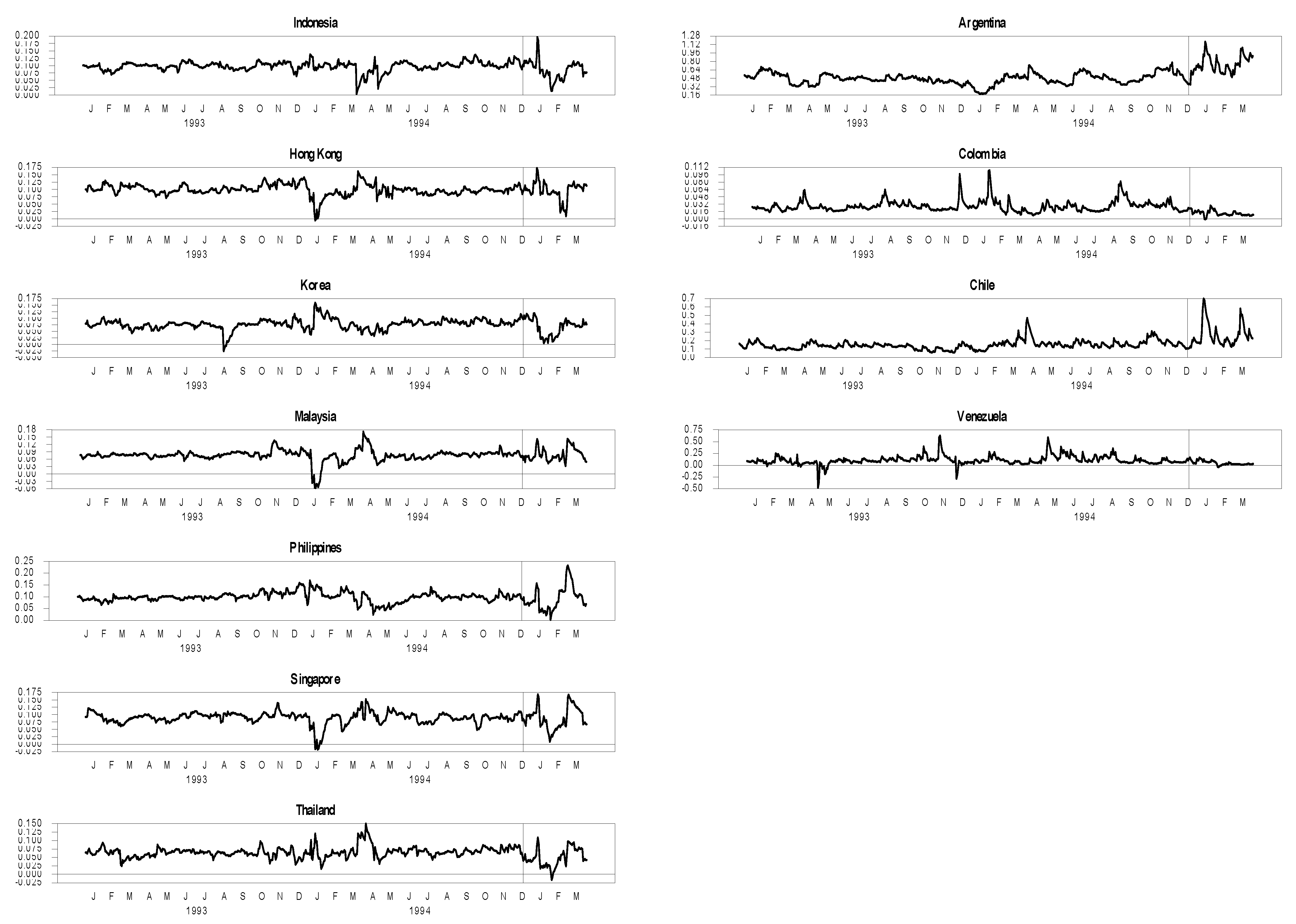
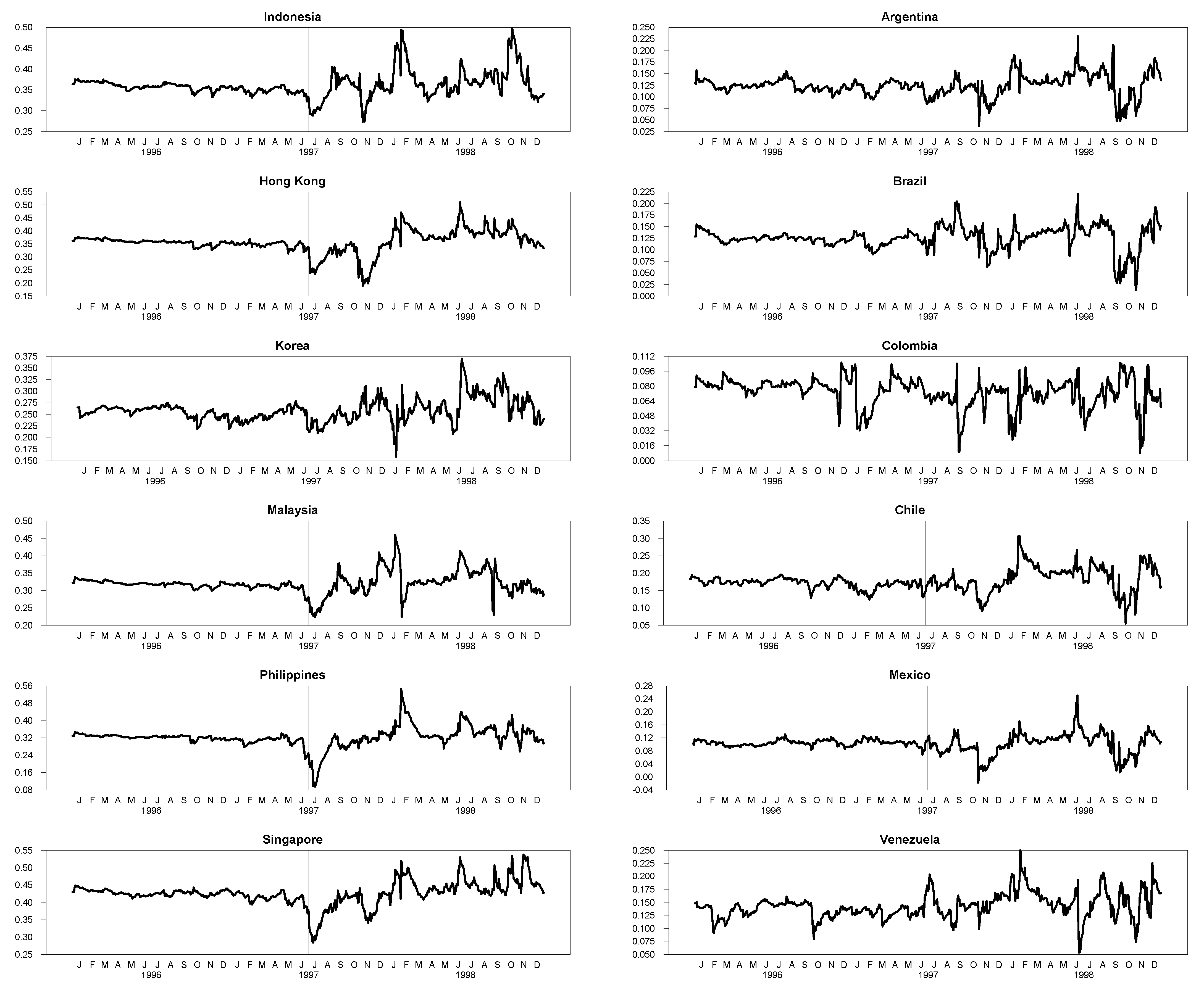
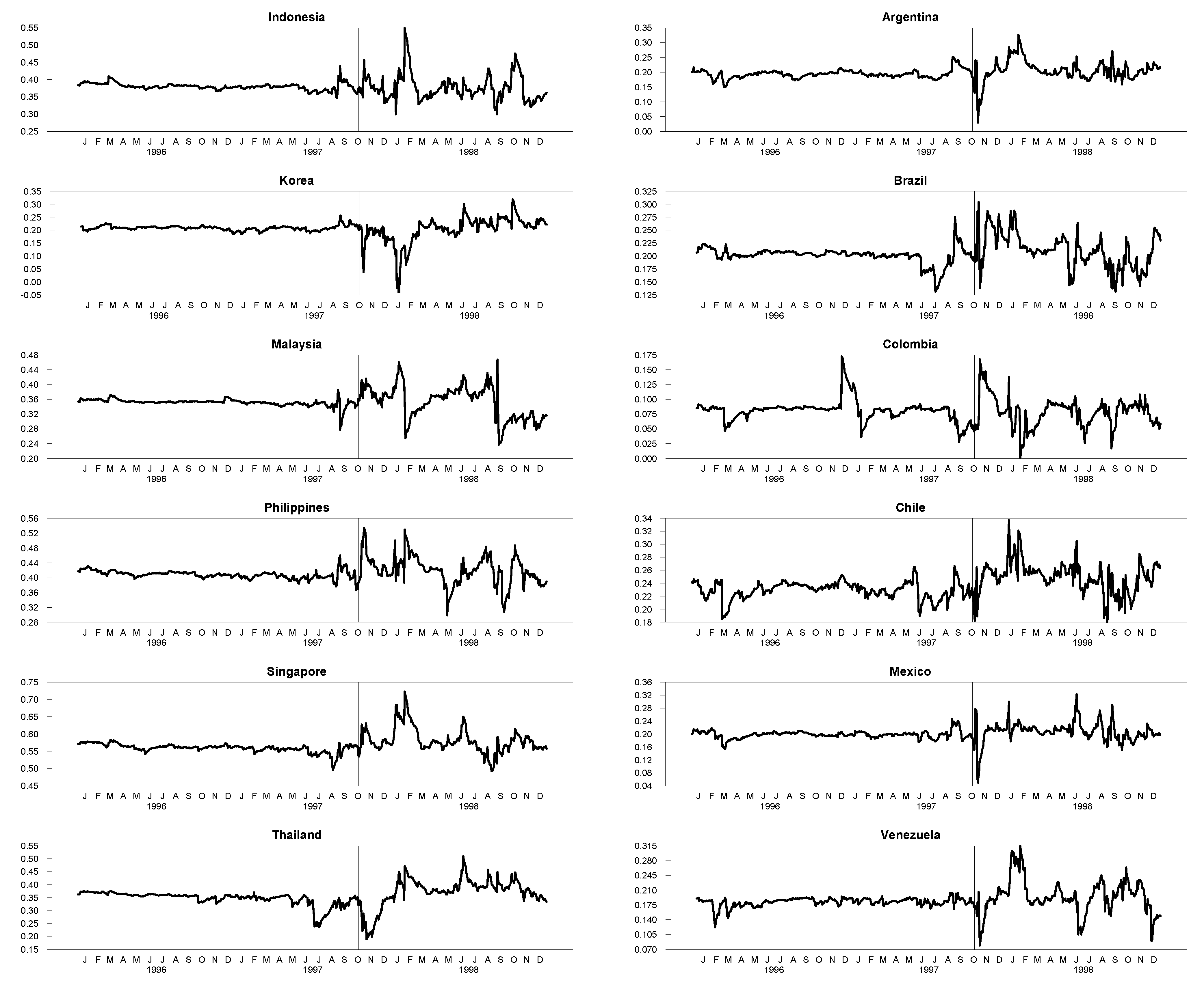
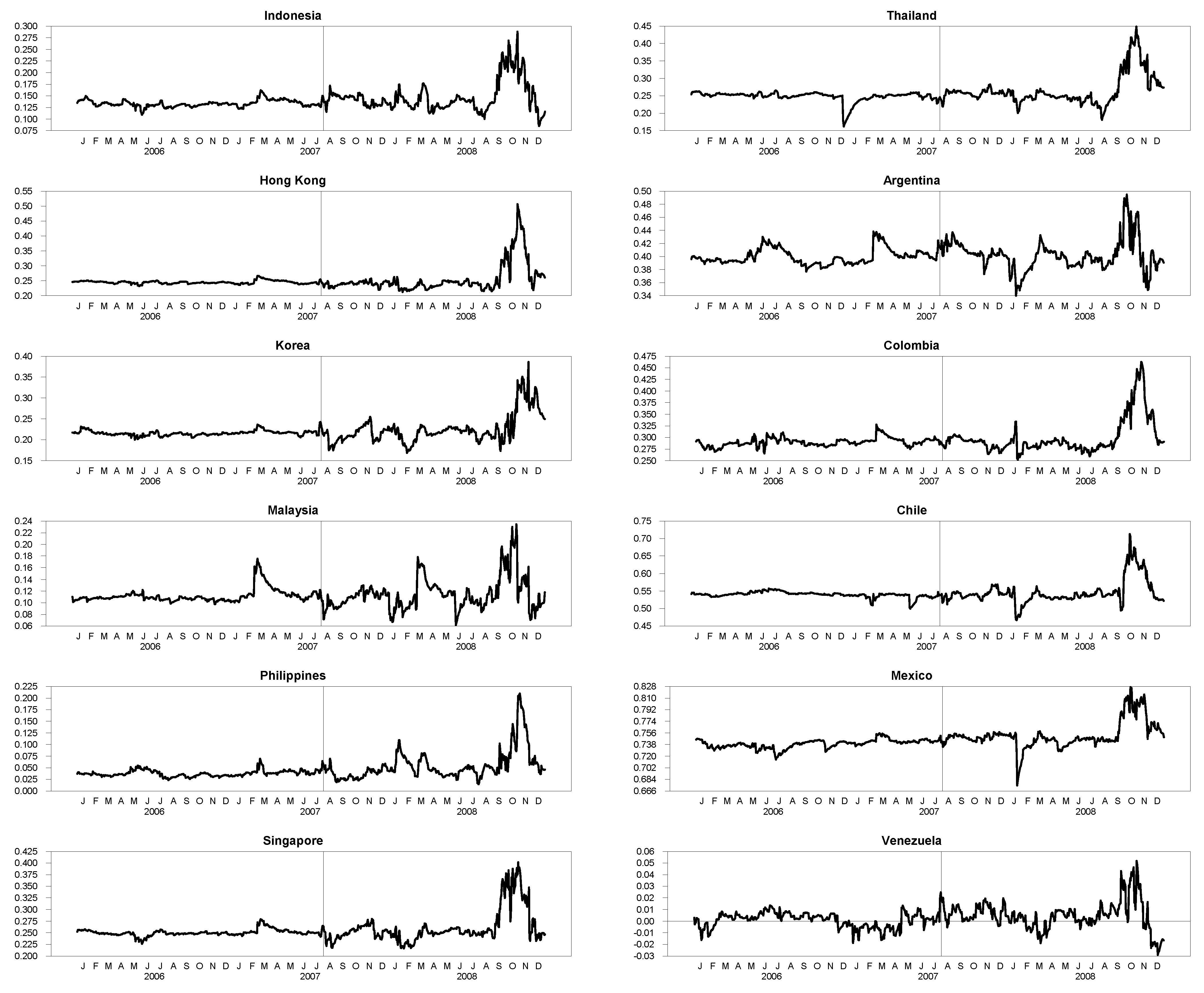
5.1. Dynamic Conditional Correlations

We now use the dynamic conditional correlation (DCC) multivariate GARCH models presented in the previous section to test whether the contagion occurred among the region’s markets during the two periods of international financial crises: the Mexican “Tequila” crisis of 1994 and the Asian “flu” crisis of 1997. Contagion from the American stock market toward emerging stock markets (consisting of Asian and Latin American markets) is also tested in the period of the US subprime crisis of 2007. One advantage of DCC GARCH models is that we can estimate the pair-wise dynamic conditional correlations for all investigated markets in a single system. In this paper, we apply three DCC-GARCH(1,1) models for three crises in order to estimate DCC for each pair of the source and target countries. The Table 5, Table 6 and Table 7 report the estimates of the returns and conditional variances equations. The AR(1) terms in mean equation are significant except for Singapore, Taiwan (during the Mexican crisis); Singapore, Taiwan and Thailand (during the Asian crisis); and Indonesia, Taiwan, Thailand, Colombia, Mexico (during US subprime crisis). The coefficient of US returns in mean equations are highly significant, which confirms the impact of the American stock market on emerging stock markets. We just do not find significant coefficients of US returns for Colombia and Mexico during the Mexican crisis. The coefficients of lagged variances and shock-square terms are all significant at 1%, which means that the volatilities of these markets are time-varying. Hence, it supports completely the GARCH(1,1) models. The estimated parameters θ 1 and θ 2 of DCC processes are all significant at 1%. The conditions that θ 1 + θ 2 < 1 are all satisfaites.
The computed dynamic conditional correlations during the three crises are presented in Figure 1, Figure 2, Figure 3 and Figure 4. The vertical continuous lines represent the break dates: 19 December 1994 for the Mexican “Tequila” crisis, 2 July 1998 for the Asian “flu” crisis (if crisis-initiating market is Thailand), 17 October 1998 (if Hong Kong) and 1 August 2007 for the US subprime crisis.
For the Mexican crisis, as shown in Figure 1, what we can observe clearly is that the Latin American stock markets exhibit higher correlations with Mexico compared to Asian stock markets. However, we cannot state increases in the correlation between crisis-originating market and target markets except for Argentina and Chile.
During the Asian crisis (Figure 2 and Figure 3), the correlations between the market originating crisis (Thailand or Hong Kong) and Asian emerging stock markets are higher compared to their correlations with Latin American emerging stock markets. Indeed, the correlations of Latin American emerging stock markets do not exceed 35% while those of Asian emerging stock markets are sometimes more than 50%. However, the DCCs of the markets of these two regions with Thailand or Hong Kong share one common characteristic: the correlations become more volatile after the crisis. There are obviously increases in these correlations beyond the break points in most cases.
The Figure 4 shows the DCCs of all emerging stock markets under investigation with the US stock market during the US subprime crisis occurred in 2007. In the early stage of the US subprime crisis, the DCCs fluctuate lightly. Then they peak around the final quarter of 2008. At that time, their values are very high, especially those with Latin American emerging stock markets. Except for Venezuela, which is less than 10%, the DCC reach at 80% for Mexico, 70% for Chile, 50% for Argentina while the highest correlation between the US stock markets and the Asian emerging stock markets is about 50% for Hong Kong. This period corresponds to the Lehman Brothers’ collapse6. Hence, the bankruptcy of Lehman Brothers seems to have the big impact on the contagion of the US subprime crisis toward the Asian and Latin American emerging stock markets. An increase in the volatility of DCCs after the crisis is also observed.

5.2. Contagion Tests

Although increases in some correlations between crisis markets and target markets during three crises have been noticed, we are not sure if they are statistically significant, which is the evidence of shift contagion. Hence, in order to test for the existence of contagion, we firstly calculate the average correlations in pre-crisis and crisis periods, and then use the t-test as presented in Section 3 to verify if the average correlation in crisis period is statistically higher than that in pre-crisis period. The results are reported in Table 8, Table 9, Table 10 and Table 11.

5.2.1. Contagion during the Mexican “Tequila” Crisis

In the Mexican “Tequila” crisis, we do not find contagion from Mexican stock market to Asian emerging stock markets. Actually, the DCCs between Indonesia, Korea and Singapore increase lightly after the crisis with respectively 0.0017%, 1.1157%, and 2.1926% (Table 8). However, these increases are not statistically significant. The t-statistics are inferior to the critical values, leading to accept the null hypothesis of non contagion. This implies an interdependence phenomen between these markets and Mexican market, and not a shift contagion. On the contrary, concerning Latin American stock markets, there is a pure contagion phenomenon from Mexican stock market to Argentinian, Chilian stock markets. The DCCs between these two markets and Mexican stock markets increased significantly at 1% between two periods. These results allow us to conclude that Mexican crisis was just a regional phenomenon. This finding is consistent with the work of Bodart and Candelon (2009).

5.2.2. Contagion during the Asian “flu” Crisis

The contagion tests from Thailand to other emerging stock markets during the Asian “flu” crisis show that there is shift contagion from the crisis-originating market to the both Asian and Latin American regions. We can see that contagion is present in all Asian emerging stock markets under investigation. For Latin American stock markets, the contagion tests demonstrate the presence of contagion in Argentina, Brazil, Chile and Venezuela. Based on the increase in DCC mean in percentage term (See Table 9), Taiwan is most influenced by contagion in Asian region7 and Venezuela in Latin American region.
In considering Hong Kong as the market originating Asian “flu” crisis instead of Thailand, we also find the presence of contagion effects in the both Asian and Latin American regions. However, the results are slightly different. For Asian emerging stock markets, the contagion effects are present in the Philippines, Singapore, Taiwan and Thailand, and not in Indonesia, Korea and Malaysia. For Latin American emerging stock markets, shift contagion phenomenon is found in most markets except Colombia.

5.2.3. Contagion during the US Subprime Crisis

As presented in Table 11, the DCCs between US and Asian emerging stock markets are generally smaller than those between US and Latin American emerging stock markets. Exceptionally, the DCCs for Philippines and Venezuela are very small compared to other markets, respectively about 5% and 1%. The highest DCC for Asian region is about 27% (for Singapore) while the highest DCC for Latin American region is more than 75% (for Mexico). However, they all show an increase after the crisis occurs. The t tests for the significant increases of DCCs between tranquil and turmoil periods lead to the rejection of non contagion for most of the markets, except Brazil. In fact, the DCCs between U.S. and Brazil increase after the crisis but it is not statistically significant. However, they are very high, respectively 71.34% and 71.46% in tranquil and crisis periods. This indicates an interdependence phenomenon between Brazil and US and not a shift contagion.

6. Conclusions

Since the international financial crises that occurred in the last two decades, there have been a variety of papers that investigate whether contagion risk is present in financial markets during the crisis periods. In fact, as observed in reality, financial shocks in one country have important impacts in other countries. This raises the question about the role of contagion in the literature. However, how to define and measure contagion is still a contentious problem.
In this paper, we use a traditional definition of contagion which indicates it as a significant increase in cross-market linkages after a shock to one country. Hence, the method applied to test for the existence of contagion in stock markets under investigation is to test if the correlations increase significantly after the crisis. The increase of cross-market correlations is the evidence of contagion risk. This approach is used in many works that deals with the problem of financial contagion risk as it is rather simple compared to other methods like including dummy variables.
We study contagion effects in emerging stock markets during the 1994 Mexican crisis, the 1997 Asian crisis and the 2007 US crisis. The sample consists of eight emerging stock markets in Asia (Indonesia, Hong Kong, Korea, Malaysia, Philippines, Singapore, Taiwan and Thailand), and six markets in Latin America (Argentina, Brazil, Chile, Colombia, Mexico, Venezuela) and the US stock market. To compute conditional correlations across markets, we apply DCC-GARCH(1,1) to daily stock index returns of all the markets in the sample for three crises. We then test for a significant increase in means of dynamic conditional correlations of target markets with source markets during crisis periods.
We find evidence for contagion risk in emerging stock markets during three crises. However, there is a difference of degree of spread among these crisis. During the Mexican crisis, there is a shift contagion from Mexico to two other markets in the same region (Argentina and Chile, all at 1%). During the Asian crisis, contagion is not only detected in Asian region but also in Latin American region. If considering Thailand as contagion source, we find evidence for contagion from Thailand to Indonesia, Hong Kong, Korea, Malaysia, Philippines, Singapore, Taiwan and Thailand (in Asia) and Argentina, Brazil, Chile, Venezuela (in Latin America), all at 1% except for Hong Kong (10%). Alternatively, if we assume that the Asian crisis was triggered by the crash of Hong Kong stock market, the results show that Philippines, Singapore, Taiwan and Thailand (in Asia) and Argentina, Brazil, Chile, Mexico, Venezuela (in Latin America) suffer contagion effects from Hong Kong, all at 1%. With respect to the US subprime crisis, we can detect support for contagion in all studied markets at 1% apart from Brazil. This confirms once again the undeniable impact of US stock market to emerging stock markets.
Among three studied crises, only the Mexican crisis in 1994 is found to be a regional phenomenon. However, this crisis occurred more than twenty years ago, when these countries had just begun their liberalization processes. Afterward, the financial crises became more contagious. Regarding the Asian crisis in 1997, contagion is also detected in the Asian and Latin American regions. The US subprime crisis in 2007 is found to be the most contagious as contagion is detected in most of studied markets in both Asian and Latin American regions. Thereby, the contagion effect seems evident in emerging stock markets in the context that these countries become more open and integrated in the global economy after their liberalization processes.
In summary, in this paper, shift contagion in emerging stock markets during crisis periods has been found present. As a result, the most important element that causes contagion effects across markets is the behavior of investors. In the literature of contagion, a shock to one market can make changes in the anticipations of investors in other markets, and hence lead to portfolio rebalancing. In the presence of information asymmetry, this may transfer the crisis to other markets. Consequently, this can be a subject for more detailed researches in the future. Besides, this paper still presents some shortcomings. The main problem of this study concerns the definition of contagion. In this paper, we consider the contagion as an increase of correlation between the markets. Moreover, we apply a simple method to detect the contagion. We use one side t-test instead of other persistent measures. Therefore, these problems must be further examined in the future.

Funding

This research received no external funding.

Conflicts of Interest

The author declares no conflict of interest.

References

  1. Baig, Taimur, and Ilan Goldfajn. 1999. Financial markets contagion in the Asian crisis. IMF Staff Papers 46: 167–95. [Google Scholar]
  2. Billio, Monica, and Loriana Pelizzon. 2003. Contagion and interdependence in stock markets: Have they been misdiagnosed? Journal of Economics and Business 55: 405–26. [Google Scholar] [CrossRef]
  3. Bodart, Vincent, and Bertrand Candelon. 2009. Evidence of interdependence and contagion using a frequency domain framework. Emerging Markets Review 10: 140–50. [Google Scholar] [CrossRef]
  4. Bollerslev, Tim, Ray Y. Chou, and Kenneth F. Kroner. 1992. ARCH modeling in finance: A review of the theory and empirical evidence. Journal of Econometrics 52: 5–59. [Google Scholar] [CrossRef]
  5. Boyer, Brian H., Michael S. Gibson, and Mico Loretan. 1997. Pitfalls in Tests for Changes in Correlations; International Finance Discussion Papers 597; Washington, DC: Board of Governors of the Federal Reserve System (U.S.).
  6. Calvo, Sara, and Carmen Reinhart. 1996. Capital Flows to Latin America: Is There Evidence of Contagion Effects? World Bank Policy Research Paper 1619. Washington, DC: World Bank. [Google Scholar]
  7. Chiang, Thomas C., Bang Nam Jeon, and Huimin Li. 2007. Dynamic correlation analysis of financial contagion: Evidence from Asian markets. Journal of International Money and Finance 26: 1206–28. [Google Scholar] [CrossRef]
  8. Cho, Jang Hyung, and Ali M. Parhizgari. 2008. East Asian financial contagion under DCC-GARCH. International Journal of Banking and Finance 6: 17–30. [Google Scholar]
  9. Corsetti, Giancarlo, Marcello Pericoli, and Massimo Sbracia. 2005. ‘Some contagion, some interdependence’: More pitfalls in tests of financial contagion. Journal of International Money and Finance 24: 1177–99. [Google Scholar] [CrossRef]
  10. Dornbusch, Rudiger, Yung Chul Park, and Stijn Claessens. 2001. Contagion: How it spreads and how it can be stopped? In International Cinancial Contagion. Boston: Klwer Academic Publishers. [Google Scholar]
  11. Engle, Robert F. 2002. Dynamic conditional correlation: A simple class of multivariate generalized autoregressive conditional heteroskedasticity models. Journal of Business and Economics Statistics 20: 339–50. [Google Scholar] [CrossRef]
  12. Engle, Robert F., and Kevin Sheppard. 2001. Theoretical and Empirical Properties of Dynamic Conditional Correlation Multivariate GARCH. NBER Working Paper No. 8554. Cambridge: National Bureau of Economic Research. [Google Scholar]
  13. Forbes, Kristin J., and Roberto Rigobon. 2002. No contagion, only interdependence: Measuring stock market comovements. Journal of Finance 57: 2223–61. [Google Scholar] [CrossRef]
  14. Forbes, Kristin, and Roberto Rigobon. 2000. Contagion in Latin America: Definitions, Measurements and Policy Implications. NBER Working Paper, No. 7885. Cambridge: National Bureau of Economic Research, September. [Google Scholar]
  15. Forbes, Kristin, and Roberto Rigobon. 2001. Measuring contagion: Conceptual and empirical. In International Fiancial Contagion. Boston: Klwer Academic Publishers. [Google Scholar]
  16. Horta, Paulo, Carlos Mendes, and Isabel Vieira. 2008. Contagion Effects of the U.S. Subprime Crisis on Developped Countries. CEFAGE-UE Working Paper No. 2008/08. Évora: University of Evora. [Google Scholar]
  17. Kaminsky, Graciela L., and Carmen Reinhart. 2000. On crises, contagion, and confusion. Journal of International Economics 51: 145–68. [Google Scholar] [CrossRef]
  18. King, Mervyn A., and Sushil Wadhwani. 1990. Transmission of volatility between stock markets. Review of Financial Studies 3: 5–33. [Google Scholar] [CrossRef]
  19. Kumar, Manmohan S., and Avinash Persaud. 2001. Pure contagion and investors’ shifting risk appetite: Analytical issues and empirical evidence. International Finance 5: 401–36. [Google Scholar] [CrossRef]
  20. Longin, Francois, and Bruno Solnik. 1995. Is the correlation in international equity returns constant: 1960–1990? Journal of International Money and Finance 14: 3–26. [Google Scholar] [CrossRef]
  21. Masson, Paul. 1998. Contagion: Monsoonal Effects, Spillovers, and Jumps between Multiple Equilibra. IMF Working Paper 98/142. Washington, DC: International Monetary Fund. [Google Scholar]
  22. Moser, Thomas. 2003. What is international financial contagion? International Finance 6: 157–78. [Google Scholar] [CrossRef]
  23. Naoui, Kamel, Naoufel Liouane, and Salem Brahim. 2010a. A dynamic conditional correlation analysis of financial contagion: The case of the subprime credit crisis. International Journal of Economics and Finance 2: 85–96. [Google Scholar] [CrossRef]
  24. Pericoli, Marcello, and Massimo Sbracia. 2003. A primer on financial contagion. Journal of Economic Surveys 17: 571–608. [Google Scholar] [CrossRef]
  25. Ramchand, Latha, and Raul Susmel. 1998. Volatility and cross correlation across major stock markets. Journal of Empirical Finance 5: 397–416. [Google Scholar] [CrossRef]
1.
The interdependence term here refers to a high level of market comovement in all periods.
2.
See Pericoli and Sbracia (2003) for a review of contagion definition.
3.
4.
5.
Problem raised by Forbes and Rigobon (2002) as discussed above.
6.
Lehman Brothers is the fourth largest U.S. Investment Bank, which filed for bankruptcy on 15 September 2008.
7.
This result is consistent with the work of Cho and Parhizgari (2008).
Figure 1. The dynamic correlation estimation for the Mexican “Tequila” crisis. The vertical continuous line represents the break date: 19 December 1994.
Jrfm 11 00089 g001
Figure 2. The dynamic correlation estimation for the Asian “flu” crisis (Source of contagion: Thailand). The vertical continuous line represents the break date: 2 July 1997.
Jrfm 11 00089 g002
Figure 3. The dynamic correlation estimation for the Asian “flu” crisis (Source of contagion: Hong Kong). The vertical continuous line represents the break date: 17 October 1997.
Jrfm 11 00089 g003
Figure 4. The dynamic correlation estimation for the US Subprime crisis. The vertical continuous line represents the break date: 1 August 2007.
Jrfm 11 00089 g004
Table 1. Descriptive statistics on stock returns: The Mexican crisis.
Stable Period
1 January 1993–16 December 1994
Turnoil Period
19 December 1994–31 March 1995
MeanStd DevSkewnessKurtosisNMeanStd DevSkewnessKurtosisN
Asian emerging markets
Indonesia0.10040.9222−0.4486 ***2.6498 ***5110.01501.0549−0.6917 **0.927075
Hong Kong0.08021.5790−0.2401 **1.7596 ***5110.05281.70430.19880.923575
Korea0.09291.26320.10091.1744 ***511−0.09951.3775−0.24450.653475
Malaysia0.08111.41400.03127.9182 ***5110.05541.52790.5262 *1.9441 ***75
Philippines0.19011.1940−0.07401.4608 ***511−0.14281.4014−0.6524 **1.1863 **75
Singapore0.05480.84290.02603.6975 ***511−0.05221.0070−1.3139 ***5.2778 ***75
Taiwan0.16951.86830.3141 ***2.2656 ***511−0.07001.26750.08631.9812 ***75
Thailand0.13441.6338−0.16103.3274 ***511−0.03961.52370.09941.1044*75
Latin American emerging markets
Argentina0.06281.7080−0.4579 ***1.7082 ***511−0.31813.48880.5977 **1.2190 **75
Chile0.14740.9804−0.1968 *1.4879 ***511−0.08931.98330.8658 ***2.1619 ***75
Colombia0.10920.82480.6607 ***4.2164 ***5110.09630.79021.8254 ***4.5397 ***75
Mexico0.05881.3187−0.05762.2076 ***511−0.24132.53920.29280.690475
Venezuela0.13562.87430.8210 ***8.0160 ***5110.02851.42871.3654 **7.0395 **75
The returns are in percentages. *, **, *** represent statistical significance at the 1%, 5%, 10% levels of risk.
Table 2. Descriptive statistics on stock returns: The Asian crisis (Source of contagion: Thailand).
Stable Period
1 January 1996–1 July 1997
Turmoil Period
2 July 1997–31 December 1998
MeanStd DevSkewnessKurtosisNMeanStd DevSkewnessKurtosisN
Asian emerging markets
Indonesia0.07821.0492−0.3121 **2.3480 ***392−0.07273.19180.2923 **3.2094 ***392
Hong Kong0.11641.0426−1.22228.9774392−0.13012.78240.41755.8187392
Korea−0.04671.35860.19100.7480 ***392−0.00603.36310.3847 ***1.1348 ***392
Malaysia0.02250.8135−0.4775 ***2.6060 ***392−0.14523.35260.6484 ***12.4451 ***392
Philippines0.04060.9691−0.19812.5731 ***392−0.08392.24710.2459 **2.1380 ***392
Singapore−0.02640.80150−0.13210.6031 **392−0.06651.89730.3777 ***3.6296 ***392
Taiwan0.16741.3831−0.00063.6794 ***392−0.07521.7950−0.03601.4828 ***392
Latin American emerging markets
Argentina0.09761.2867−0.16731.9277 ***392−0.07632.3432−0.5134 ***6.2535 ***392
Brazil0.17660.95400.148303.4620 ***392−0.18112.4182−0.6825 ***3.1787 ***392
Chile0.02520.69370.4481 ***0.5236 **392−0.11791.11950.13553.4237 ***392
Colombia0.05871.0545−0.7724 ***47.0383 ***392−0.08001.0778−0.00399.7246 ***392
Mexico0.11780.91330.5029 ***1.6971 ***392−0.03801.73650.02137.6136 ***392
Venezuela0.34571.67061.0121 ***3.7608 ***392−0.18662.78411.1492 ***12.5781 ***392
The returns are in percentages. **, *** represent statistical significance at the 5%, 10% levels of risk.
Table 3. Descriptive statistics on stock returns: The Asian Crisis (Source of contagion: Hong Kong).
Stable Period
1 January 1996–16 October 1997
Turnoil Period
17 October 1997–31 December 1998
MeanStd DevSkewnessKurtosisNMeanStd DevSkewnessKurtosisN
Asian emerging markets
Indonesia0.01661.42800.6768 ***12.7077 ***469−0.01783.32120.17582.8525 ***315
Hong Kong0.06631.2338−0.7219 ***7.0780 ***469−0.11572.95680.4178 ***5.3991 ***315
Korea−0.10331.38250.03130.9223 ***4690.08823.67600.3107 **0.5446 *315
Malaysia−0.03671.26731.5841 ***25.3818 ***469−0.09813.52740.5284 ***12.0150 ***315
Philippines−0.03521.2483−0.3863 ***7.4819 ***469−0.00152.26800.2740 **1.9341 ***315
Singapore−0.03930.9059−0.2921 **1.8088 ***469−0.05722.01500.4080 ***3.3187 ***315
Taiwan0.11631.4502−0.11102.5102 ***469−0.05841.81050.00311.9019 ***315
Thailand−0.14932.02190.6848 ***3.3557 ***469−0.10543.23930.7468 ***2.1230 ***315
Latin American emerging markets
Argentina0.10201.2704−0.18311.7405 ***469−0.12552.5457−0.4468 ***5.2178 ***315
Brazil0.15301.1524−0.3935 ***6.2960 ***469−0.23352.5350−0.6586 ***2.9229 ***315
Chile0.00410.68800.4351 ***0.5212 **469−0.12151.20740.12942.8595 ***315
Colombia0.08500.9906−0.8211 ***50.7480 ***469−0.15301.16040.12928.7253 ***315
Mexico0.13220.95120.3708 ***1.2385 ***469−0.09751.85160.08657.1560 ***315
Venezuela0.32401.61120.9646 ***3.8058 ***469−0.28443.03531.1840 ***10.8894 ***315
The returns are in percentages. *, **, *** represent statistical significance at the 1%, 5%, 10% levels of risk.
Table 4. Descriptive statistics on stock returns: The US subprime Crisis.
Stable Period
1 January 2006–31 July 2007
Turnoil Period
1 July 2007–31 December 2008
MeanStd DevSkewnessKurtosisNMeanStd DevSkewnessKurtosisN
Asian emerging markets
Indonesia0.15221.2398−0.7613 ***4.3101 ***411−0.15252.3802−0.4674 ***4.1386 ***371
Hong Kong0.12020.9329−0.7289 ***2.4423 ***411−0.14912.52150.05623.1464 ***371
Korea0.07241.0974−0.4801 ***1.3515 ***411−0.13972.2650−0.2754 **4.6030 ***371
Malaysia0.10430.7091−1.2220 ***7.4879 ***411−0.12261.2308−1.3304 ***10.6139 ***371
Philippines0.13111.1670−0.863 ***5.8259 ***411−0.17111.7675−0.6680 ***5.8814 ***371
Singapore0.10810.8867−0.9309 ***2.9231 ***411−0.19021.8069−0.18603.0287 ***371
Taiwan0.06651.0303−0.87863.1950 ***411−0.18041.9659−0.05100.8381 ***371
Thailand0.04881.5232−2.8566 ***53.3222 ***411−0.17982.1168−0.6096 ***5.6193 ***371
Latin American emerging markets
Argentina0.08821.0504−0.9743 ***5.9111 ***411−0.11131.3972−0.0210 ***3.3975 ***371
Brazil0.13651.2836−0.3056 **1.5830 ***411−0.11212.4737−0.02782.9948 ***371
Chile0.11520.7406−1.1789 ***5.9941 ***411−0.07881.37210.5007 ***7.4257 ***371
Colombia0.03331.6017−0.070212.4863 ***411−0.03121.4454−0.4301 ***6.7485 ***371
Mexico0.13591.1573−0.17523.0393 ***411−0.08281.72430.3276 **3.6350 ***371
Venezuela0.12471.5929−3.0199 ***33.0170 ***411−0.07580.67300.5511 ***3.1822 ***371
US stock market
US0.03970.6747−0.5250 ***2.5716 ***411−0.12682.2007−0.14915.2257 ***371
The returns are in percentages. **, *** represent statistical significance at the 5%, 10% levels of risk.
Table 5. Estimation of DCC-GARCH model for the Mexican “Tequila” crisis.
r t = γ 0 + γ 1 r t 1 + γ 2 r t 1 U S + ε t
h t = ω + α ε t 1 2 + β h t 1
Q t = ( 1 θ 1 θ 2 ) Q ¯ + θ 1 ν t 1 ν t 1 + θ 2 Q t 1
Parameter γ 0 γ 1 γ 2 ω α β
Asian emerging markets
Indonesia0.0629 ***0.2630 ***0.2332 ***0.4799 ***0.2687 ***0.2094 **
(2.6687)(8.7874)(6.6515)(6.9350)(5.2765)(2.4816)
Korea−0.00160.0926 ***0.09440.0748 ***0.0586 ***0.8927 ***
(−0.0453)(2.8503)(1.6300)(2.8749)(4.2400)(34.4931)
Malaysia0.0466 **0.0656 ***0.3697 ***0.0417 ***0.0752 ***0.8974 ***
(1.9780)(2.8854)(8.9527)(3.1666)(5.2569)(44.3229)
Philippines0.0709 **0.1821 ***0.2813 ***0.0176 ***0.0458 ***0.9394 ***
(2.3330)(5.7971)(5.2114)(2.7262)(4.3183)(72.2894)
Singapore0.0113−0.00980.2945 ***0.1085 ***0.1297 ***0.7113 ***
(0.6121)(−0.3630)(8.4910)(4.8621)(5.0067)(15.1351)
Taiwan0.0413−0.03240.2365 ***0.1313 ***0.0628 ***0.8874 ***
(0.8180)(−1.0263)(2.7341)(3.1662)(5.1356)(38.8341)
Hong Kong0.0502 *−0.0493 *0.7935 ***0.0117 ***0.0444 ***0.9503 ***
(1.7065)(−1.7108)(18.8004)(2.8495)(7.5667)(168.3592)
Thailand0.02110.0780 **0.4172 ***0.0372 **0.0674 ***0.9193 ***
(0.6028)(2.5041)(6.6277)(2.1545)(4.9942)(50.8437)
Latin American emerging markets
Argentina0.05540.0738 ***0.3022 ***0.1122 ***0.0865 ***0.8827 ***
(1.2221)(2.6945)(4.0964)(3.1756)(5.2608)(41.3832)
Chile0.02010.2549 ***0.0988 **0.0595 ***0.1957 ***0.7527 ***
(0.8533)(8.9928)(2.3914)(5.4924)(8.2280)(28.7125)
Colombia−0.01750.4280 ***−0.01620.0700 ***0.2050 ***0.6914 ***
(−1.1340)(11.8014)(−0.6823)(7.4205)(7.5636)(21.9471)
Venezuela0.03340.1197 ***0.1559 *0.4403 ***0.3591 ***0.6256 ***
(0.5934)(3.7851)(1.7650)(5.1880)(7.3100)(15.6333)
Mexico0.0748 **0.1240 ***0.08670.0540 ***0.0772 ***0.8957 ***
(2.1861)(4.4517)(1.4082)(2.9099)(4.7209)(41.8666)
θ 1 = 0.0091 *** (2.5764); θ 2 = 0.8750 *** (9.7801). Note: Italic numbers in parentheses are t-statistics. *, **, *** represent statistical significance at the 1%, 5%, 10% (p value) of parameters.
Table 6. Estimation of DCC-GARCH model for the Asian “flu” crisis.
r t = γ 0 + γ 1 r t 1 + γ 2 r t 1 U S + ε t
h t = ω + α ε t 1 2 + β h t 1
Q t = ( 1 θ 1 θ 2 ) Q ¯ + θ 1 ν t 1 ν t 1 + θ 2 Q t 1
Parameter γ 0 γ 1 γ 2 ω α β
Asian emerging markets
Indonesia0.07380.1152 ***0.4308 ***0.0355 ***0.1043 ***0.9056 ***
(1.6114)(5.2387)(9.4292)(2.9913)(7.1851)(79.3786)
Hong Kong0.1029 ***0.0702 ***0.6562 ***0.0500 ***0.1086 ***0.8900 ***
(2.9622)(−2.6696)(16.3620)(3.7141)(6.8789)(58.8206)
Korea0.01530.0932 ***0.2868 ***0.0276 **0.0725 ***0.9281 ***
(0.2672)(2.7627)(5.1863)(1.9922)(6.8351)(89.4653)
Malaysia0.0484 *0.0590 **0.3088 ***0.0128 ***0.1229 ***0.8934 ***
(1.6858)(1.9972)(8.1332)(3.2957)(8.8803)(97.8157)
Philippines0.04940.1459 ***0.3143 ***0.1023 ***0.2091 ***0.7831 ***
(1.4304)(4.9254)(8.4482)(5.1229)(7.7183)(32.4725)
Singapore0.04950.00860.3732 ***0.0344 ***0.0715 ***0.9202 ***
(1.5878)(−0.3252)(9.9155)(3.0880)(4.9210)(58.3597)
Taiwan0.0989 **0.02590.2771 ***0.1180 **0.0662 ***0.8918 ***
(2.0661)(0.7897)(6.2478)(2.5499)(4.3803)(33.6636)
Thailand0.03210.03440.3467 ***0.0913 ***0.1073 ***0.8932 ***
(−0.5486)(1.0719)(4.8863)(2.5801)(6.7971)(61.1801)
Latin American emerging markets
Argentina0.0967 **0.0681 ***0.0867 **0.2440 ***0.1284 ***0.8076 ***
(2.4066)(2.6343)(2.1024)(5.6291)(7.4994)(35.4268)
Brazil0.1461 ***0.0513 **0.1783 ***0.1234 ***0.1427 ***0.8349 ***
(4.1852)(2.1644)(4.6334)(4.8453)(6.7531)(37.5869)
Chile0.02070.2515 ***0.0852 ***0.0241 ***0.0764 ***0.8968 ***
(0.8866)(9.0373)(3.8795)(3.4661)(5.2825)(51.0718)
Colombia0.01280.2275 ***0.0769 ***0.1084 ***0.2233 ***0.7303 ***
(−0.8760)(9.8500)(3.9644)(6.2665)(5.9507)(21.8016)
Mexico0.1073 ***0.0873 ***0.1191 ***0.0968 ***0.1067 ***0.8522 ***
(3.2568)(3.4749)(3.4945)(3.9108)(6.5547)(38.7641)
Venezuela0.02530.2219 ***0.2545 ***0.2062 ***0.2084 ***0.7679 ***
(0.4845)(6.6611)(4.5883)(4.6099)(6.4188)(26.0453)
θ 1 = 0.0100 *** (5.1374); θ 2 = 0.9204 *** (52.0098). Note: Italic numbers in parentheses are t-statistics. *, **, *** represent statistical significance at the 1%, 5%, 10% (p value) of parameters.
Table 7. Estimation of DCC-GARCH model for the US Subprime crisis.
r t = γ 0 + γ 1 r t 1 + γ 2 r t 1 U S + ε t
h t = ω + α ε t 1 2 + β h t 1
Q t = ( 1 θ 1 θ 2 ) Q ¯ + θ 1 ν t 1 ν t 1 + θ 2 Q t 1
Parameter γ 0 γ 1 γ 2 ω α β
Asian emerging markets
Indonesia0.2265 ***−0.03710.4390 ***0.1915 ***0.1371 ***0.8175 ***
(5.7232)(−1.3703)(14.8630)(2.7140)(3.9892)(16.3024)
Korea0.1426 ***−0.0591 ***0.4602 ***0.0451 ***0.0677 ***0.9227 ***
(4.2410)(−2.7507)(16.6541)(3.7266)(6.3664)(80.1653)
Malaysia0.1051 ***0.02450.2148 ***0.0277 ***0.1524 ***0.8425 ***
(5.5955)(0.9712)(15.0682)(3.1640)(6.1689)(30.6932)
Philippines0.1073 ***0.0432 **0.4816 ***0.1307 ***0.2038 ***0.7557 ***
(3.6841)(2.0841)(24.7262)(4.1638)(7.1927)(24.0974)
Singapore0.1526 ***−0.1309 ***0.4332 ***0.0370 ***0.0719 ***0.9157 ***
(5.7167)(−7.1061)(19.0871)(5.9154)(9.3246)(110.2176)
Taiwan0.1129 ***−0.03510.4178 ***0.0308 ***0.0490 ***0.9431 ***
(3.2060)(−1.4837)(16.4201)(3.0436)(5.1028)(80.4188)
Hong Kong0.1726 ***−0.0933 ***0.5775 ***0.0474 ***0.0915 ***0.9057 ***
(5.4715)(−5.1091)(21.4708)(4.6845)(8.9123)(92.2507)
Thailand0.1680 ***−0.03290.3372 ***1.0153 ***0.2215 ***0.4901 ***
(4.2402)(−1.2364)(11.6561)(4.5281)(4.2943)(4.7025)
Latin American emerging markets
Argentina0.1442 ***0.03750.1114 ***0.1799 ***0.0746 ***0.8276 ***
(4.0163)(1.1469)(4.2305)(4.9710)(4.8060)(27.1994)
Brazil0.2432 ***−0.1042 ***0.1159 ***0.0944 ***0.0599 ***0.9090 ***
(6.2098)(−5.2976)(3.4103)(4.1900)(6.3348)(62.2301)
Chile0.1276 ***0.0995 ***0.0496 ***0.0650 ***0.1224 ***0.8094 ***
(5.6065)(3.8369)(2.9036)(5.0398)(6.9301)(31.73603)
Colombia0.1238 ***0.03700.1040 ***0.1820 ***0.2388 ***0.6475 ***
(4.2682)(1.0867)(5.4842)(7.4010)(8.2245)(20.6911)
Mexico0.1784 ***−0.01440.0521 ***0.0569 ***0.0611 ***0.9105 ***
(5.7761)(−0.6505)(1.8097)(4.2185)(6.6728)(67.41723)
Venezuela−0.01110.1535 ***0.0535 ***0.1026 ***0.5049 ***0.5477 ***
(−0.7179)(5.7888)(4.4745)(5.8995)(9.9013)(14.22591)
US0.0946 ***−0.1055 *** 0.0199 ***0.0823 ***0.9067 ***
(3.7963)(−3.8855) (4.8415)(8.6645)(88.7960)
θ 1 = 0.0086 *** (4.3979); θ 2 = 0.9211 *** (34.2800). Note: Italic numbers in parentheses are t-statistics. *, **, *** represent statistical significance at the 1%, 5%, 10% (p value) of parameters.
Table 8. Results of contagion test in emerging stock markets: The Mexico “Tequila” crisis in 1994.
Stable Period
1 January 1993–16 December 1994
Turnoil Period
19 December 1994–31 March 1995
MeanStd DevNMeanStd DevNMean Increase (%)t StatictisContagion
Asian emerging markets
Korea0.07750.01975110.06680.031675−13.7570−2.8409N
Malaysia0.07620.02355110.08020.0261755.26831.2577N
Philippines0.09890.01985110.09330.050975−5.6818−0.9455N
Singapore0.08970.02025110.08910.037775−0.6939−0.1401N
Taiwan0.04250.01535110.03550.037075−16.4346−1.6127N
Thailand0.06590.01565110.04910.027475−25.5032−5.1963N
Latin American emerging markets
Argentina0.47340.68805110.74060.17177556.464313.1390C ***
Chile0.14940.38655110.26380.13817576.55467.1045C ***
Colombia0.02790.16695110.01260.005675−54.8510−18.0838N
Venezuela0.10700.32715110.04900.045675−54.1615−8.6066N
*** represents statistical significance at the 10% level of risk. N: No contagion; C: Contagion.
Table 9. Results of contagion test in emerging stock markets: The Asian “flu” crisis in 1997 (Contagion source: Thailand).
Stable Period
1 January 1996–1 July 1997
Turnoil Period
2 July 1997–31 December 1998
MeanStd DevNMeanStd DevNMean Increase (%)t StatictisContagion
Asian emerging markets
Indonesia0.35590.00973920.36730.04113923.20735.3562C ***
Hong Kong0.35470.01163920.35930.05863921.29971.5284C *
Korea0.25290.01293920.26400.03143924.36606.4443C ***
Malaysia0.31750.00923920.32520.04043922.41803.6650C ***
Philippines0.31820.01663920.32660.06153922.66632.6372C ***
Singapore0.42300.01203920.42980.04723921.60022.7536C ***
Taiwan0.14750.00013920.16650.001539212.87599.2121C ***
Latin American emerging markets
Argentina0.12280.01123920.12670.03023923.16832.3918C ***
Brazil0.12310.01083920.12900.03383924.80543.2968C ***
Chile0.17140.01403920.18540.04063928.19826.4719C ***
Colombia0.07840.01263920.06880.0172392−12.2519−8.9302N
Mexico0.10450.00883920.10120.0365392−3.1670−1.7448N
Venezuela0.13410.01423920.15130.028739212.830810.6444C ***
*, *** represent statistical significance at the 1%, 10% levels of risk. N: No contagion; C: Contagion.
Table 10. Results of contagion test in emerging stock markets: Asian “flu” crisis in 1997 (Contagion source: Hong Kong).
Stable Period
1 January 1996–16 October 1997
Turnoil Period
17 October 1997–31 December1998
MeanStd DevNMeanStd DevNMean Increase (%)t StatictisContagion
Asian emerging markets
Indonesia0.38020.00944690.37660.0379315−0.9470−1.6517N
Korea0.20860.00894690.20230.0518315−3.0045−2.1265N
Malaysia0.35170.00904690.35240.04423150.19750.2748N
Philippines0.40800.01054690.41990.03903152.89815.2614C ***
Singapore0.55990.01184690.58070.03623153.71749.8697C ***
Taiwan0.23360.01574690.24990.04863156.95475.7406C ***
Thailand0.34680.02524690.37230.05583157.34277.5909C ***
Latin American emerging markets
Argentina0.19390.01364690.20560.03533156.02265.6008C ***
Brazil0.20160.01534690.21020.03423154.30504.2230C ***
Chile0.22970.01314690.24940.02373158.571413.4455C ***
Colombia0.08110.01754690.07810.0251315−3.7808−1.8855N
Mexico0.19830.01114690.20710.03063154.42704.8752C ***
Venezuela0.19830.01114690.20710.03063154.42705.1917C ***
*** represents statistical significance at the 10% level of risk. N: No contagion; C: Contagion.
Table 11. Results of contagion test in emerging stock markets: The US subprime crisis in 2007.
Stable Period
1 January 2006–31 July 2007
Turnoil Period
1 August 2007–31 December 2008
MeanStd DevNMeanStd DevNMean Increase (%)t StatictisContagion
Asian emerging markets
Indonesia0.13370.00734110.14680.03243719.82247.6402C ***
Hong Kong0.24510.00534110.25550.04943714.23024.0262C ***
Korea0.21590.00584110.22550.03503714.44305.2203C ***
Malaysia0.11190.01164110.11470.02833712.49371.7711C **
Philippines0.03780.00674110.05480.033237145.03319.6879C ***
Singapore0.25020.00694110.26170.03713714.62215.9123C ***
Taiwan0.12330.00564110.13260.02743717.49186.3644C ***
Thailand0.24850.01434110.26510.04433716.67076.8943C ***
Latin American emerging markets
Argentina0.39980.63234110.40160.02373710.44241.2989C *
Brazil0.71340.84474110.71460.03503710.15620.6085N
Chile0.54010.73494110.54630.03503711.15363.3411C ***
Colombia0.29010.53864110.29970.03863713.31374.6816C ***
Mexico0.73910.85974110.75230.02123711.791411.5450C ***
Venezuela0.00080.02904110.00480.0125371472.06855.4992C ***
*, **, *** represent statistical significance at the 1%, 5%, 10% levels of risk. N: No contagion; C: Contagion.

