Urban Surface Ozone Concentration in Mainland China during 2015–2020: Spatial Clustering and Temporal Dynamics

Abstract

Urban ozone (O₃) pollution in the atmosphere has become increasingly prominent on a national scale in mainland China, although the atmospheric particulate matter pollution has been significantly reduced in recent years. The clustering and dynamic variation characteristics of the O₃ concentrations in cities across the country, however, have not been accurately explored at relevant spatiotemporal scales. In this study, a standard deviational ellipse analysis and multiscale geographically weighted regression models were applied to explore the migration process and influencing factors of O₃ pollution based on measured data from urban monitoring sites in mainland China. The results suggested that the urban O₃ concentration in mainland China reached its peak in 2018, and the annual O₃ concentration reached 157 ± 27 μg/m³ from 2015 to 2020. On the scale of the whole Chinese mainland, the distribution of O₃ exhibited spatial dependence and aggregation. On the regional scale, the areas of high O₃ concentrations were mainly concentrated in Beijing-Tianjin-Hebei, Shandong, Jiangsu, Henan, and other regions. In addition, the standard deviation ellipse of the urban O₃ concentration covered the entire eastern part of mainland China. Overall, the geographic center of ozone pollution has a tendency to move to the south with the time variation. The interaction between sunshine hours and other factors (precipitation, NO₂, DEM, SO₂, PM_2.5) significantly affected the variation of urban O₃ concentration. In Southwest China, Northwest China, and Central China, the suppression effect of vegetation on local O₃ was more obvious than that in other regions. Therefore, this study clarified for the first time the migration path of the gravity center of the urban O₃ pollution and identified the key areas for the prevention and control of O₃ pollution in mainland China.

1. Introduction

Ozone (O₃), an important trace component of the natural atmosphere, is formed by the photochemical reaction of nitrogen oxides (NO_x) and hydrocarbons in the atmosphere after being irradiated by ultraviolet light [1,2]. Studies have shown that long-term exposure to high concentrations of O₃ in the atmosphere not only directly destroys the lung function and visual function of local residents, but also affects thyroid function and nervous and cardiovascular systems [3,4,5]. Many researchers have confirmed that O₃ in the near-surface atmosphere poses a significant threat to the health of organisms. For example, a 10 ppb increase in 1-day ozone was associated with a 1.56% increase in emergency department and urgent care visits in the Washington, DC metropolitan area [6]. In the entire Northern Hemisphere, O₃ pollution in the troposphere exhibits an increasing trend, especially in South and East Asia [7,8,9,10]. On the regional scale, the long-term dynamic evolution of near-ground O₃ has not been systematically revealed. Therefore, it is necessary to research the dynamic evolution process and spatial distribution characteristics of near-ground O₃ in order to control urban O₃ pollution, and this goal motivates this study.

O₃ pollution in the atmosphere has become increasingly prominent on a national scale in mainland China in the last two decades. Mainland China is not only one of the most densely populated areas in the world, but is also one of the fastest-growing areas of industrialization and urbanization. Studies have shown that in the past two decades, near-ground O₃ pollution in various regions of mainland China has been increasing, and the health of more and more residents are threatened by O₃ pollution [11,12,13,14]. Feng et al. concluded that the O₃ concentration increased by 62.40% during particulate pollution episodes in Beijing (BTH) in the autumn from 2013 to 2015 [15]. Gao et al. analyzed the O₃ Monitoring Instrument (OMI) satellite data and suggested that the O₃ concentration in northeastern China rose from 81.3 to 87.4 μg/m³ during 2015–2018, and the nonattainment days kept increasing [16]. Xu et al. showed that under the influence of the southeast monsoon, O₃ pollution in Shanghai became particularly serious when anthropogenic contaminants were mixed with biological volatile organic compounds [17]. Numerous studies have reported the level and distribution characteristics of O₃ pollution in major metropolitan areas in mainland China. However, the spatial clustering and temporal dynamics of O₃ concentration have not been systematically clarified for the entire mainland of China.

Cities are concentrated and sensitive areas of O₃ pollution [18]. On the one hand, gaseous pollutants of NO_x and volatile organic compounds (VOC_S), which are precursors of O₃, mainly come from industrial activities and automobile exhaust [19,20]. On the other hand, ozone emitted in cities and suburbs concentrate inside cities along with urban heat island circulation, causing aggravation of ozone pollution in upper atmospheric layers [21,22]. In addition, both human and natural factors affect the migration behavior and dynamic variations of urban O₃ pollution. Factors such as the atmospheric particulate matter concentration, gaseous pollutant concentration, urban traffic conditions, temperature inversion, wind speed, temperature, hours of sunlight, humidity etc. have significant effects on the formation and concentration levels of O₃ [23,24,25]. However, most studies on the influence of factors on O₃ pollution focused only on individual urban areas, while the influence of these factors on O₃ has not been revealed on a national scale. In addition, hypothesis that the rugged terrain and variable vegetation of mainland China may have an impact on the migration and diffusion of O₃.

Considering the above-mentioned reasons, this study explores the characteristics of spatial clustering and temporal dynamics of the O₃ concentration in cities from mainland China on a long-term scale. We also distinguish the effects of topography and vegetation characteristics on the distribution of O₃ in various regions of China. To achieve these goals, the rest of this work contains three subsequent steps: (1) the analysis of the spatiotemporal distribution of the urban O₃ concentration in mainland China from 2015 to 2020; (2) the characterization of the clustering and dynamic evolution of the urban O₃ concentration at both the national and regional scales; and (3) the clarification of the influence of different typical environmental factors on the O₃ concentration in various regions in China.

2. Materials and Methods

2.1. Data Collection

The analysis of long-term and high-precision O₃ concentration data helps to clarify the spatiotemporal distribution and evolution characteristics of urban O₃ pollution in mainland China. We adopted the daily maximum 8-h average (MDA 8) O₃ concentration from 1550 monitoring stations from 336 cities in mainland China spanning from 2015 to 2020. All monitoring sites were derived from urban sites, and non-urban air monitoring sites were excluded from this study. To control the validity of the data, we strictly followed the minimum requirements for statistical validity of O₃ concentration data as stipulated in the Ambient Air Quality Standards (GB3095-2012) for statistical analysis. In addition, we have also taken into account the adverse effects of anomalous values at individual monitoring stations at a given moment in time. For this reason, we counted 8-h average concentration data for O₃ containing the following two criteria: (1) at least 6 h of average concentration values were included; and (2) the difference between the individual moments of the same monitoring point does not exceed one times the minimum value over a period of six consecutive periods. Monitoring data that did not meet this requirement were excluded.

The O₃ concentration data were collected from the national real-time city’s air quality release platform in the China National Environmental Monitoring Center (http://106.37.208.233:20035/ (accessed on 30 July 2021)). Meteorological factor data were derived from the National Meteorological Information Center (NMIC) of the China Meteorological Administration (http://data.cma.cn/ (accessed on 15 August 2021)), and the normalized vegetation index (NDVI) was obtained from the Resource and Environment Science Data Center of the Chinese Academy of Sciences (http://www.resdc.cn/ (accessed on 10 September 2021)). Detailed data types and sources are shown in Table S1, in Supplementary Materials.

2.2. Methodology

2.2.1. Spatial Autocorrelation Analysis

Spatial autocorrelation analysis is a method to explore the spatial distribution pattern, the degree of spatial dependence, and the potential spatial dependence of spatial variables at different locations. It is widely used in the research of air pollution [26,27]. In this study, the global spatial autocorrelation statistics (Moran’s index) were calculated to explore the spatial agglomeration characteristics of O₃ distribution in cities in mainland China. Geoda 2.0 software (Chicago, IL, USA) was used to calculate the global Moran’s index, and after 999 Monte Carlo simulation tests, statistical tests were performed using the standardized statistic Z (test level α = 0.05). The local indications of spatial association (LISA) were used to identify the spatial concentration of O₃ in a local area. The calculation and significance test formulas for global spatial autocorrelation and local spatial autocorrelation are shown in Equations (1)–(3):

$$I_{G\mathrm{lobal}}=\frac{\mathrm{n}{\displaystyle \sum _{\mathrm{i}=1}^{\mathrm{n}}{\displaystyle \sum _{j=1}^n{W}_{ij}(x_i-\overline{x}})(x_j-\overline{x})}}{{\displaystyle \sum _{i=1}^n{\displaystyle \sum _{j=1}^n{W}_{ij}{\displaystyle \sum _{i=1}^n{(x_i-\overline{x})}^2}}}}$$

(1)

$$Z=\frac{I-E(I)}{\sqrt{VAR(I)}}$$

(2)

$$I\mathrm{Local}=\frac{(x_i-\overline{x})}{{\displaystyle \sum _i{(x_i-\overline{x})}^2}}{\displaystyle \sum _j{W}_{ij}(x_i-\overline{x})}$$

(3)

In these equations, I is the Moran’s index; n is the number of cities; x_i and x_j are the O₃ concentration of the i-th and j-th cities, respectively; $\overline{\mathrm{x}}$ is the average of the O₃ concentration in cities; n is the number of cities; W_ij is the spatial weight matrix; VAR(I) represents the variance of the global Moran’s index; and E(I) represents the expected value of the Moran’s index.

2.2.2. Hot Spot Analysis

Hot spot analysis was used to identify statistically significant spatial clustering characteristics of high values (representing hot spots) and low values (cold spots). The results (z score and p value) can be used to identify the spatial clustering locations of high- and low-valued elements. This method considers the characteristics of O₃ in the neighboring areas. This method is of great significance in revealing the spatial clustering characteristics of atmospheric pollutants. Using this method, the Getis-Ord Gi* statistic was adopted to calculate each value of the O₃ concentration. The Z score was used to test Gi*. Among them, if the z score > 1.96, it indicated that there was a high-value cluster or hot spot area of O₃; if the z score < −1.96, it indicated that there was a low-value cluster or cold spot area of O₃. The formula of Gi* is shown in Equations (4)–(6):

$$\overline{X}=\frac{{\displaystyle \sum _{j=1}^n{x}_j}}{n}$$

(4)

$$S=\sqrt{\frac{{\displaystyle \sum _{j=1}^n{x}_j{}^2}}{n}}-{(\overline{X})}^2$$

(5)

$$G{i}^{\ast }=\frac{{\displaystyle \sum _{j=1}^n{W}_{ijxj}-\overline{X}{\displaystyle \sum _{j=1}^n{W}_{ij}}}}{\sqrt[s]{\frac{[n{\displaystyle \sum _{j=1}^n{W}^2{}_{ij}-({\displaystyle \sum _{j=1}^n{W}_{ij}{)}^2}}}{n-1}}}$$

(6)

where, S is the standard deviation of the O₃ concentration, and the other parameters are the same as those in Equations (1)–(3).

2.2.3. Standard Deviational Ellipse Analysis (SDE)

The function of SDE is to quantitatively describe geographic elements with the center, long axis, and short axis as the basic parameters [28]. The center of the SDE indicates the spatial distribution characteristics of the elements and their relative positions in space, and the long and short axes can reflect the spatial distribution of the elements. In this study, the spatial distribution and movement characteristics of O₃ distribution in mainland China cities were revealed through the variation in the center of gravity, long axis, and short axis of the SDE. The formula of SDE is expressed by Equations (7)–(9).

$${\overline{X}}_w=\frac{{\displaystyle \sum _{i=1}{w}_i}{x}_i}{{\displaystyle \sum _{i=1}^n{w}_i}}$$

(7)

$${\sigma }_x=\frac{\sqrt{{\displaystyle \sum _{i=1}^n\left(w_i{x}_i\cos \theta -w_i\overline{y_i}\sin \theta \right)}}}{{\displaystyle \sum _{i=1}^n{w}_i^2}}$$

(8)

$${\sigma }_y=\frac{\sqrt{{\displaystyle \sum _{i=1}^n\left(w_i{\overline{x}}_i\sin \theta -w_i{\overline{y}}_i\cos \theta \right)}}}{{\displaystyle \sum _{i=1}^n{w}_i^2}}$$

(9)

In the equations, (x_i, y_i) is the spatial region of the research object; w_i is the weight; i is the decision-making unit; x and y represent the relative coordinates of each point from the center of the standard deviation ellipse, respectively; θ is the rotation angle of the distribution pattern; and σ_x and σ_y are the standard deviations of the x-axis and y-axis, respectively.

2.2.4. Multiscale Geographically Weighted Regression Model (MGWR)

Compared with the classical geographic weighted regression model (GWR), the MGWR allows each variable to have a different spatial smoothing level, which can reduce the estimation error. The MGWR therefore is a further optimization and improvement of the GWR. It can optimize the specific bandwidths of each independent variable’s relationship with the dependent variable. Based on the preliminary estimation results of GWR, it can decide on an optimal influencing scale using the backward fitting technology to obtain a more accurate result [29]. The equation of MGWR is shown in Equation (10).

$$y_i={\beta }_0\left(u_i,v_i\right)+{\displaystyle \sum _{j=1}^k{\beta }_{bwj}\left(u_i,v_i\right)x_{ij}}+{\epsilon }_i$$

(10)

In Equation (10), (u_i, v_i) are the coordinates of the local sampling location; β₀ is the bandwidth of intercept, and the subscript “bwk” denotes the bandwidth of variable k; β_bwj is the regression coefficient of the j-th variable at i; and ε_i is the random error at (u_i, v_i).

In this study, the GWR estimation is used as the initial estimation. Subsequently, the difference between the true value and the predicted value obtained by the initialization estimation is calculated, which represents the initialization residual ($\widehat{\epsilon }$) described by Equation (11):

$$\hat{\epsilon }=y-{\displaystyle \sum _{j=1}^k{\hat{f}}_j} (f_j={\beta }_{bwj}{x}_j)$$

(11)

When the degree of change in the estimated value of the regression coefficient is less than 1 × 10⁻⁵, the model fitting is considered to be completed and the calculation stops. In this study, all variables were standardized before the model fitting. The calculation of the MGWR is based on the MGWR2.2 software (https://sgsup.asu.edu/SPARC (accessed on 25 September 2021)) developed by the Spatial Analysis Research Center (SPARC) of Arizona State University, USA, and the map production is completed by the ArcGIS10.6 software (Redlands, CA, USA).

2.2.5. Multi-Factor Generalized Additive Model (MGAM)

MGAM is a free nonparametric regression model that can flexibly represent complex relationships between variables and freely detect the effects of nonlinear regression [30]. A smooth function is used to fit each feature in the model. Furthermore, the model automatically selects the appropriate polynomial to explain the relationship between the independent and dependent variables. The equation of MGAM is shown in Equation (12).

$$\mathrm{y}={\beta }_0+f_j\left(K_1\right)+f_j\left(K_2\right)+f_j\left(K_3\right)+\cdots +f_j\left(K_N\right)$$

(12)

In Equation (12), y is the O₃ concentration in the study area, β₀ is the intercept of the model, K₁, K₂, K₃… K_N are the main environmental factors, and f_j (K) is the smooth function of K₁, K₂, K₃… K_N.

3. Results and Discussion

3.1. Temporal Distribution Characteristics of O₃ Concentration in Cities

3.1.1. Interannual Variation of Urban O₃ Concentration

The 90th percentile of MDA8 in mainland China in 2015–2020 is listed in

Table 1. Statistical data of the 90th percentile of the MDA8 from urban monitoring stations in mainland China (2015–2020) (µg/m³) ^#.

Year	Counts	Min	Max	Mean	Coefficient of Variation (%)
2015	1491	42	227	142 ± 29	20.52
2016	1462	54	228	146 ± 27	18.52
2017	1425	35	236	156 ± 29	18.78
2018	1489	25	230	157 ± 27	16.92
2019	1579	32	225	152 ± 27	17.98
2020	1550	60	211	143 ± 24	17.10

^# MDA8, representing the annual mean O₃ concentration of the maximum daily 8 h average.

. The O₃ concentration of cities in mainland China exhibited an increasing trend from 2015 to 2018, and then turned into a decreasing trend after 2018. Among them, the urban O₃ concentration increased by 6.84% from 2016 to 2017. The coefficient of variation of the urban O₃ concentration in all years exceeded 10% (Table 1), indicating that the O₃ concentration did not distribute uniformly at the monitoring sites, and that there might be characteristics of aggregation.

Furthermore, the O₃ concentration in mainland China was higher than that of Europe, Iran, and India (Table S2). In particular, the average frequency of high O₃ concentration days (>160 µg/m³) in mainland China is significantly higher than that of the above-mentioned regions/countries. Studies have shown that the formation of urban O₃ was due to the emission of NO_x and VOCs, which have undergone complex photochemical reactions in the air; on the other hand, the formation of O₃ was induced by meteorological conditions such as high temperatures, strong solar radiation, and low relative humidity [31,32,33]. Compared with the above-mentioned countries/regions, the high urban O₃ concentration in mainland China was due to the development of industry, the increase in the number of automobiles, and the rapid expansion of urban areas in the last two decades. The development of cities not only aggravated the emission of NO_x and VOCs [34], but also increased the temperature of the ground surface and the probability of temperature inversion in local areas [35].

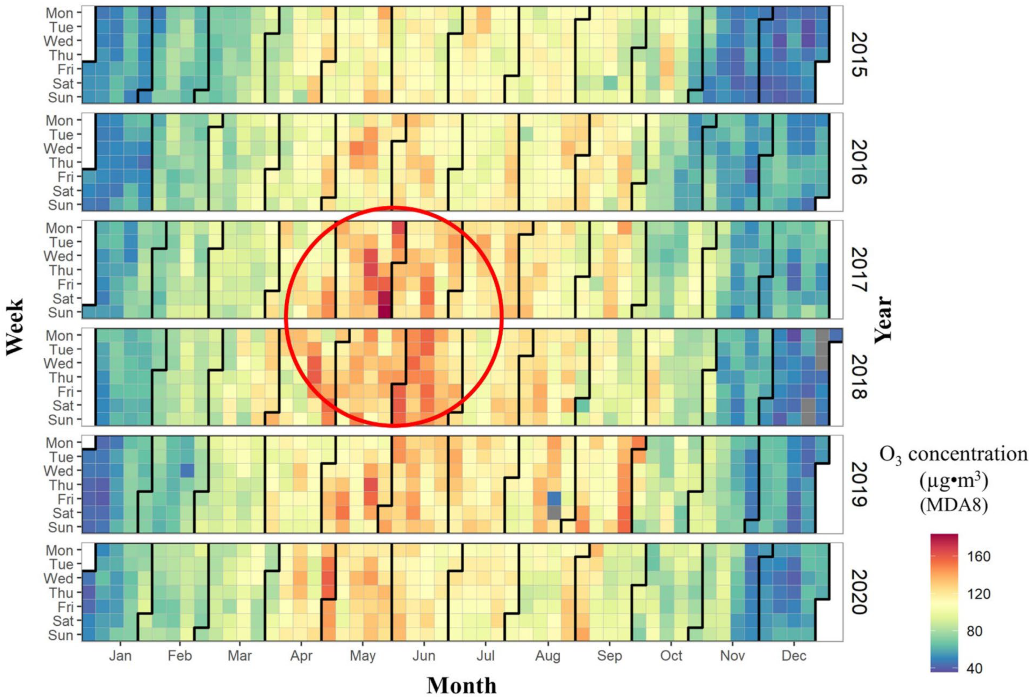
3.1.2. Monthly and Daily Variations of Urban O₃ Concentration

The monthly and daily variations of the urban O₃ concentration in mainland China from 2015 to 2020 are shown in Figure 1. On the monthly time scale, the O₃ concentration in November, December, and January was lower than that in other months, while the O₃ concentration in April, May, June, July, and August was higher than that in other months. The variations in the O₃ concentration have obvious seasonal characteristics (summer > spring > autumn > winter). The strong exchange between the stratosphere and the troposphere led to increased O₃ concentrations in spring and summer [36]. In addition, strong solar radiation generated a large number of hydroxyl radicals in the atmosphere, which stimulated the reaction of VOC and hydroxyl radicals to generate O₃ [37,38]. Compared to summer, in autumn and winter the atmospheric troposphere was relatively stable, and precipitation decreased, which slowed down the dilution and diffusion of air pollutants. In addition, weaker solar radiation also slowed down the production of O₃ in autumn and winter. However, the change of the O₃ concentration in May should be the focus of attention: the period from May to June in 2017 and 2018 was the time with the highest O₃ concentration in mainland China. On the daily time scale, the urban O₃ concentration exceeded the ambient air quality standards of China on 17 May (162 µg/m³), 18 May (165 µg/m³), 27 May (179 µg/m³), 28 May (183 µg/m³), 29 May (165 µg/m³), 2017, and 23 May 2019 (162 µg/m³) (grade II 160 µg/m³) (GB 3095-2012). The aforementioned phenomenon suggested that the urban O₃ concentration has clustering characteristics on the monthly and daily scales.

Two factors have contributed to the concentration of peak urban near-ground-level ozone concentrations in May and June. On the one hand, NO_x emissions from industrial agglomerations were elevated in May and June compared to other time periods [39]. On the other hand, the possibility of precursor phototransformation has been exacerbated by both the gradual increase in temperature and the increase in the duration of light.

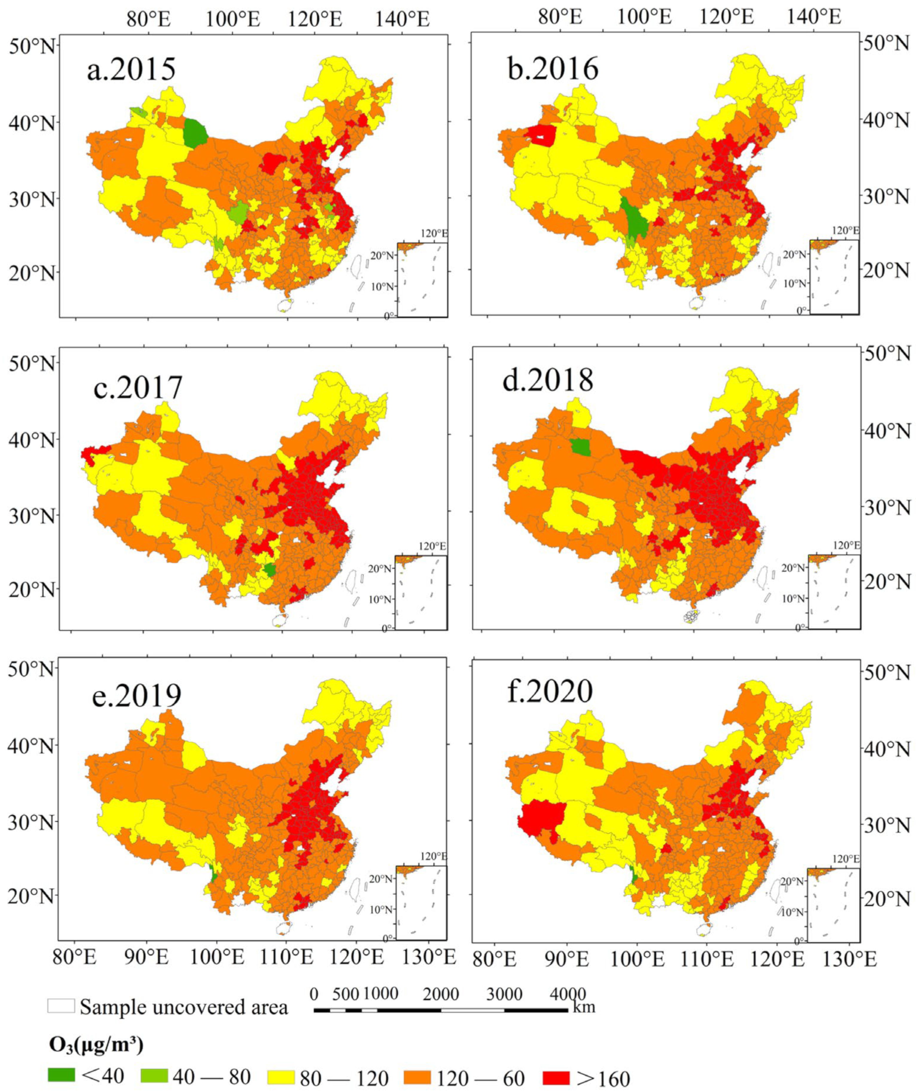
3.2. Spatial Distribution Characteristics of Urban O₃ Concentration

The trend analysis tool was used to perform a three-dimensional perspective analysis based on the urban O₃ concentration and geographic spatial coordinate projection of mainland China (Figure 2). In the east-west direction (shown by the green line in Figure 2), the best-fit trendline of the urban O₃ concentration presented a “J-shaped” curve, where the urban O₃ concentration showed a trend of low in the west and high in the east. In the north-south direction (blue line in Figure 2), the best-fit curve presented an “inverted U-shaped” curve, where the urban O₃ concentration in the mid-latitude regions of mainland China was higher than that in the low- and high-latitude regions. From a national perspective, the overlapping regions of the eastern coastal and mid-latitude regions (N30°~N40°) of mainland China were the key areas of urban O₃ pollution from 2015 to 2020.

Based on the data of urban monitoring points, the detailed spatial distribution characteristics of the urban O₃ concentration are plotted in Figure 3. From 2015 to 2016, the urban O₃ concentration pollution area exhibited a spot-like distribution, mainly concentrated in the Beijing-Tianjin-Hebei region, Shandong Peninsula, and the Yangtze River Delta region (Figure 3a,b). However, by 2018, the polluted area expanded from a spot-like shape to a surface-like shape. The areas of high O₃ concentration included most cities in North China, East China, and Central China, and even cities in Southwest China were also polluted by O₃ (Figure 3c,d). From 2018 to 2020, the area of O₃ pollution was significantly reduced, and it was confined to North China and a small part of the Yangtze River Delta (Figure 3e,f). For instance, since 2017, the near-ground O₃ concentration in the Yangtze River Delta region has shown a downward trend, which was due to the concentrations of O₃ precursors (NO_x and VOCs) emitted in 2017, which were at their peak during this time period. High concentrations of NO_x and VOCs directly contribute to elevated urban O₃ concentrations [39]. The results showed that although the concentration of O₃ in cities from mainland China has been at a high level, the degree and area of pollution are decreasing. The obvious regional aggregation characteristics of urban O₃ pollution can also be found in Figure 3. The core areas of pollution were mainly concentrated in the North China Plain and the Yangtze River Delta. From 2015 to 2018, the expansion of the O₃ pollution area in cities in China was affected by the reduction of atmospheric particulate matter (PM_2.5) and NO_x emissions [40]. Studies revealed that the reduction of PM_2.5 concentrations in the atmosphere slowed down the aerosol sink of hydroperoxyl-free radicals, thus promoting the production of O₃ [41]. In addition, the increase in temperature and the decrease in humidity on the urban surface also exacerbated the increase in the urban O₃ concentration [41]. From 2019 to 2020, the reduction in the extent of urban O₃ pollution was due to the strengthened management and control of air pollutant emissions by the government and the impact of the COVID-19 epidemic [42,43].

3.3. The Clustering Characteristics of Urban O₃ Concentration

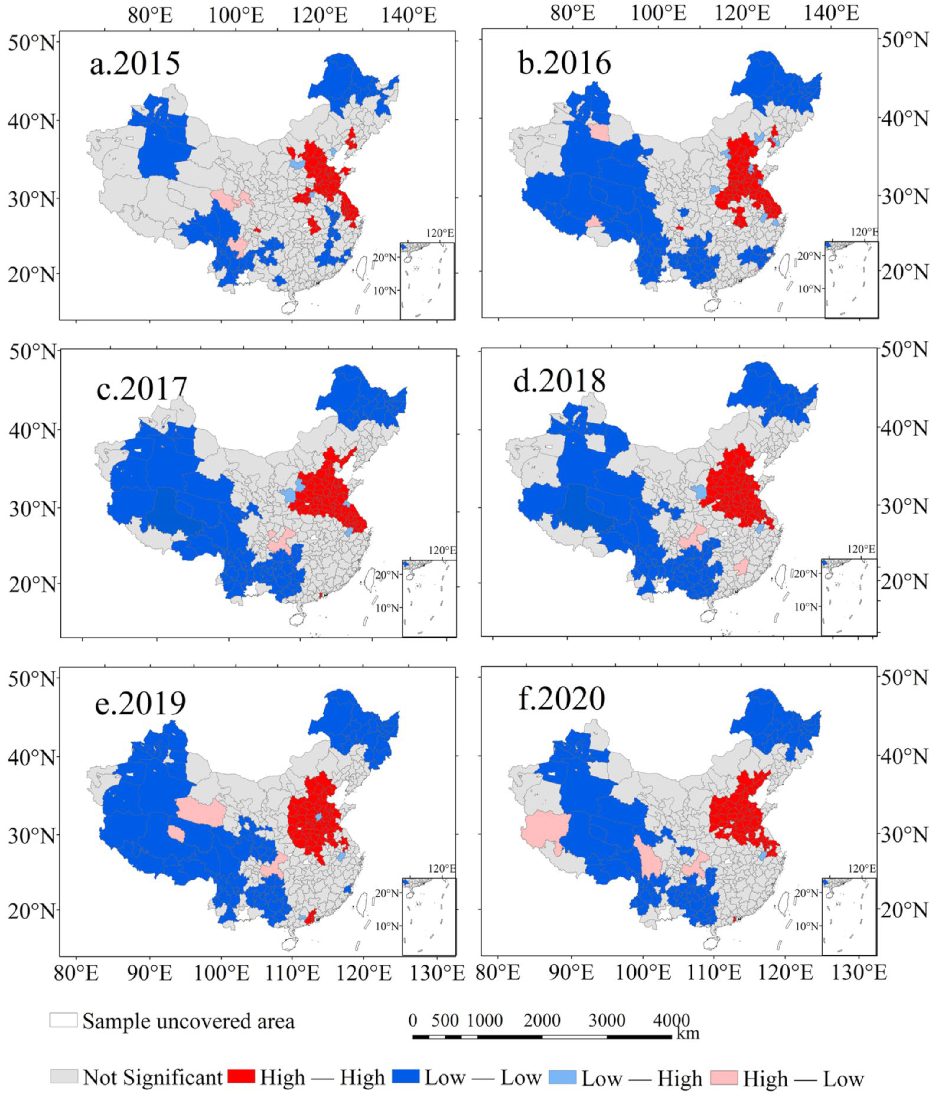
3.3.1. The Spatial Autocorrelation Characteristics of Urban O₃ Concentration

From 2015 to 2020, the distribution of the urban O₃ concentration in mainland China had significant spatial clustering characteristics (

Table 2. Results of spatial autocorrelation analysis of the urban O₃ concentration in mainland China.

Year	Moran’s I	E(I)	Z-Score	p-Value	Cluster	V(I)
2015	0.4908	−0.0030	14.1395	0.0001	Yes	0.0050
2016	0.6137	−0.0031	17.8051	0.0001	Yes	0.0032
2017	0.7496	−0.0030	21.5970	0.0001	Yes	0.0022
2018	0.7613	−0.0030	21.6733	0.0001	Yes	0.0021
2019	0.7538	−0.0030	21.7992	0.0001	Yes	0.0021
2020	0.7053	−0.0030	20.4490	0.0001	Yes	0.0024

). The difference in the global Moran’s index of O₃ distribution was statistically significant (p < 0.01, and Z > 2.58). The results indicated that urban O₃ distribution from 2015 to 2020 had a significant spatial positive correlation. The probability of the O₃ distribution showing randomness was less than 0.0001, and the clustering probability of the O₃ distribution was much greater than the probability of random distribution (Table 2). Overall, the distribution of O₃ has the characteristics of spatial dependence and aggregation. In addition, compared with the O₃ distribution characteristics in other years, the spatial clustering characteristics of the O₃ concentration in 2018 were the most obvious (Moran’s I = 0.7496).

A local spatial autocorrelation analysis (LISA) was used to analyze the spatial distribution characteristics of the O₃ concentrations in different local area units in mainland China (Figure 4). The results showed that the spatial distribution of urban O₃ presented the clustering characteristics of the same type in different regions (namely, the high-concentration area was adjacent to the high-concentration area (H-H), and the low-concentration area was adjacent to the low-concentration area (L-L)). Among them, the H-H distribution areas were mainly concentrated in Beijing-Tianjin-Hebei, Shandong, Jiangsu, Henan, and other regions. It has been confirmed that O₃ pollution was exacerbated by an interaction of atmospheric pollutants (PM₁₀, NO₂, CO, SO₂, and PM_2.5) and meteorological elements (average wind speed, sunshine duration, evaporation, precipitation, and temperature) in metropolitan areas [25]. Therefore, there are three main reasons for the concentration of O₃ in these areas. Firstly, these areas have a large population, rapid economic development, and a large number of motor vehicles, which have promoted a large amount of NO_x emissions. Secondly, compared with other regions in China, industrial enterprises such as petrochemicals, coal-fired power plants, and organic chemical industries gather in these places, resulting in more VOCs being emitted into the atmosphere [25,44]. Finally, the intense solar radiation and high temperatures in metropolitan areas in summer directly induce the photochemical behavior of O₃; in addition, the urban thermal circulation retards the dispersion of atmospheric pollutants. The L-L area was mainly concentrated in the southwestern region (such as Tibet, Xinjiang, Yunnan, and Guizhou province) and the northeastern region of China (such as Heilongjiang and Jilin provinces). The reason for the low concentration of clustering in the southwest is that NO_x and VOCs emissions were less than in other regions. In the northeast, the emission time of O₃ precursors was short and the photochemical reaction was weak, and hence most areas in this region exhibited the characteristics of low concentration clustering.

Hot spot analysis was used to further verify the accuracy of local spatial clustering of O₃ (Figure S2). The results showed that the area of O₃ clustering was wider than that calculated by LISA, and the clustering regions included North China, East China, and Central China. Moreover, from 2015 to 2020, the variations in the regions of urban O₃ clustering were not obvious, and the clustering regions had been concentrated in the above-mentioned regions. Overall, the hot spot analysis showed that the clustering area of O₃ was basically consistent with the results of the LISA analysis.

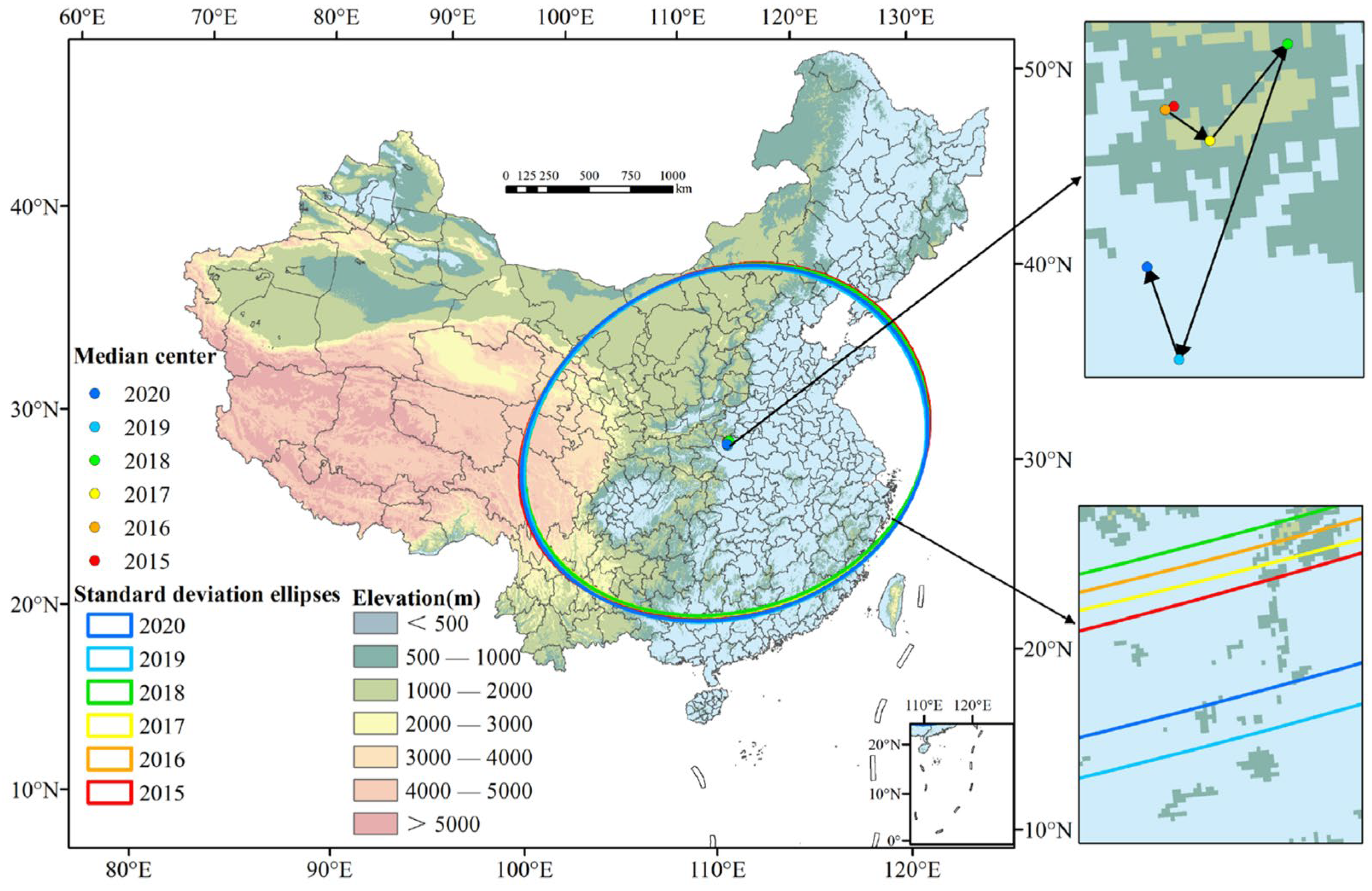
3.3.2. Spatiotemporal Evolution Pattern of Urban O₃ Concentration

To further investigate the characteristics of spatial clustering and temporal variation of the O₃ concentration, a standard deviation ellipse analysis (SDE) was used (Figure 5). In general, the standard deviation ellipse of the urban O₃ concentration covered the entire eastern part of mainland China, and the long axis of the ellipse showed a southwest-northeast trend. It is noteworthy that the direction of the long axis was basically parallel to the Chinese population boundary (Hu line), indicating that human activities played a leading role in the increasing O₃ concentrations. In addition, parts of the southwest and northwest regions of China were also included in the ellipse. The occurrence of this phenomenon may be related to the emission of air pollutants in Western China and the diffusion of pollutants in the atmosphere.

From 2015 to 2020, the length of the long and short axes of the standard deviation ellipse changed, and the mean center also moved (Figure S3 and Table S3). The length of the long axis and the short axis had both shortened and then elongated from 2015 to 2020. The combination of Figure 4 and Table S3 shows that, from 2015 to 2017, the area of the standard deviation ellipse had shrunk from 3,944,147.97 km² to 3,835,207.67 km². Subsequently, from 2018 to 2020, the area of the standard deviation ellipse had shown an expanding trend from 3,848,261.55 km² to 3,921,629.37 km². The results indicated that urban O₃ in mainland China presented a phenomenon of high concentration clustering and low concentration diffusion from 2015 to 2020. In addition, the geographic center of ozone pollution (mean center of the standard deviation ellipse) was in Nanyang City, Henan Province. The movement direction of the geographic center was first northeast and then southwest; among them, its maximum moving distance was 36.80 km from north to south and 27.84 km from east to west. Overall, the mean center tended to move to the south. This phenomenon implied that the reduction of the atmospheric O₃ concentration in North China played an important role in the prevention and control of national O₃ pollution. The emission control of O₃ precursors in urban agglomerations in southern China (e.g., Yangtze River Delta, Pearl River Delta, etc.) are conducive to the reduction of urban O₃ concentrations.

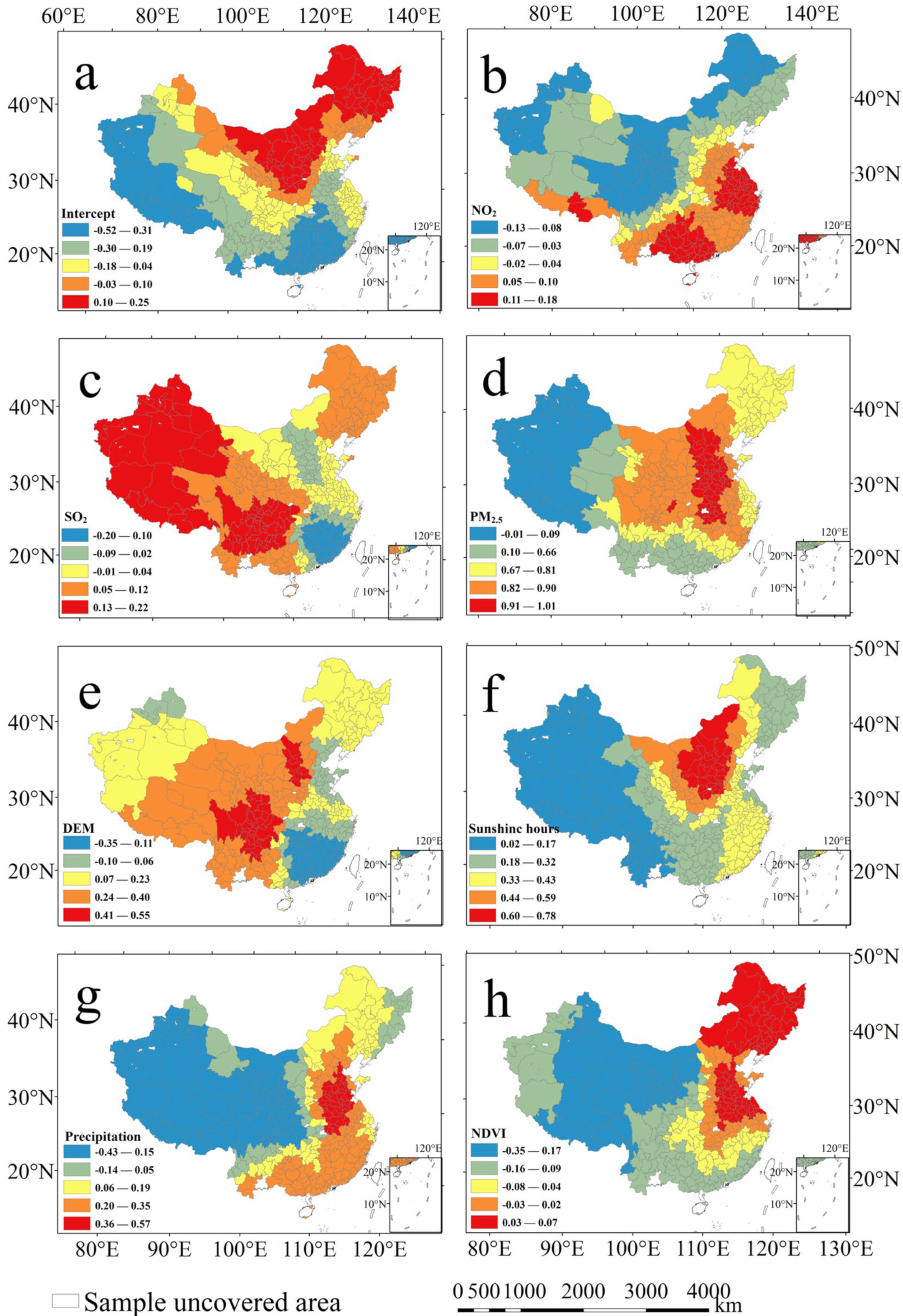
3.4. Factors Influencing the Distribution Characteristics of Urban O₃ Concentration

After multiple covariance testing and PCA analysis, NO₂, SO₂, PM_2.5, CO, DEM, temperature, sunshine hours, precipitation and NDVI were then respectively used as explanatory variables and were substituted into the OLS, GWR and MGWR model for fitting. Model fitting results show that the value of R² fitted by the MGWR model was higher than that of the OLS and GWR models, and the AIC value of MGWR fitting was lower than the AIC value of OLS and GWR fitting. The results indicated that compared with OLS and GWR, the MGWR model was more suitable for analyzing the influencing factors of the O₃ concentration in 2018 (Table S4). By the calculation of MGWR, it was found that the regression coefficients of the NO₂ concentration, the SO₂ concentration, the PM_2.5 concentration, Digital Elevation Model (DEM), sunshine hours, precipitation, and NDVI were significant overall. The regression coefficients of the other four variables (air pressure, wind speed, air temperature, and relative humidity) were not statistically significant. Among them, the concentration of SO₂, PM_2.5, DEM, sunshine hours, and precipitation were mainly positively correlated with the spatial distribution of O₃, while NDVI were negatively correlated with the spatial distribution of O₃ (Figure S4). On the spatial scale, emissions of atmospheric gas pollutants may contribute to urban O₃ formation, and the precursors of secondary particulate matter in PM_2.5, which also contains ozone precursors, can contribute to urban O₃ concentrations. There is a certain relationship between the photochemical oxidation of SO₂ and O₃. A high O₃ concentration greatly promotes the chemical conversion of SO₂ to sulfate [25]. Meteorological influences play an important role in influencing troposphere ozone concentrations, but the dominant factors show different effects on ozone in different regions [45,46]. The duration of light and the amount of evaporation are related to solar radiation. Intense solar radiation (sunshine hours) drives active photochemical reactions, which increase urban ozone concentrations. Similarly, solar radiation is stronger at higher altitudes than at lower altitudes due to the weakening effect of clouds and water vapor at lower altitudes that exacerbate the solar radiation. In addition, the effect of vegetation on regional O₃ pollution is also very closely related. Studies have shown that during drought, vegetation is less effective in removing O₃ through stomata than during wet periods, exacerbating the extreme effects of O₃ pollution [47].

Bandwidth directly reflected the spatial scale of different influencing factors in the spatial process [48,49]. The bandwidth value (BW) had a positive correlation with the spatial influence of the dependent variable. In other words, the larger the BW, the wider the influence range of the influencing factors on the independent variables; meanwhile, the spatial influence of the influence factor was similar and the spatial heterogeneity was smaller [46]. The NO₂ concentration (BW 314), DEM (BW 298), and sunshine hours (BW 318) had a wide range of effects on the spatial distribution of O₃, and the scope of their influence spread to the scale of the entire study area (Table S4). The concentration of SO₂ (BW 150), PM_2.5 (BW 56), precipitation (BW 108), and NDVI (BW 132) had an impact on the spatial distribution of urban O₃ on a local scale, and their influence had not spread to the entire study area.

Furthermore, the spatial pattern of different influencing factors on O₃ was analyzed (Figure 6). In East China, South China, Central China, and North China, the NO₂ concentration and the spatial distribution of O₃ showed a positive correlation (Figure 6b). On the one hand, these places had always been the main population distribution areas in China. Strong human activities (e.g., vehicle emissions, fossil fuel combustion, and industrial emissions) caused the emission of NO_x and VOCs. On the other hand, these regions are in low- and mid-latitude regions in China, and radiation and light stimulated the formation of O₃. Studies have shown that tropospheric O₃ is a secondary pollutant produced by the photochemical reaction of NO_x and VOCs [50]. Therefore, solar radiation, NO_x concentration, and VOCs concentration directly determined the local O₃ concentration. However, the correlation between the O₃ concentration and the NO₂ concentration in Northwest China, Northeast China, and Southwest China was not obvious, because the local emissions of VOCs and solar radiation were relatively small. The results showed that the variations of O₃ in these areas were affected by other factors. In the southwest, northwest, and northeast regions of mainland China, urban SO₂ concentration and O₃ concentration showed a positive correlation (Figure 6c). The above-mentioned areas are the main coal-burning areas in mainland China, and the SO₂ emitted during the coal-burning process is an important part of secondary inorganic aerosols [51]. However, in Eastern China, the relationship between O₃ concentration and SO₂ concentration was not obvious, which indicated that SO₂ was not the main factor influencing urban O₃ pollution in mainland China. Generally speaking, the concentration of PM_2.5 directly affected the local O₃ concentration in the entire mainland of China. The main component of PM_2.5 was composed of gaseous pollutants (such as carbon, organic carbon compound, sulfate, nitrate etc.) [52]. Among them, a minority of the chemical composition of PM_2.5 derived from direct emissions from pollution sources, and most of it originates from atmospheric photochemical transformations of SO₂, NO_x and VOCs [53]. NO_x and VOCs were the precursors of O₃ formation. Therefore, the O₃ concentration and PM_2.5 concentration had a mutual influence relationship, especially in North China, Central China, and Northwest China, where the local PM_2.5 concentration and O₃ concentration showed a clear positive correlation (Figure 6d).

On the time scale, the correlation between PM_2.5 and O₃ concentration in different seasons was further analyzed. Under the effect of different meteorological elements, the influence of PM_2.5 concentration on O₃ concentration was a complex process; however, urban PM_2.5 and O₃ concentrations showed a significant negative correlation in all seasons on the time scale. A significant negative correlation (r = −0.423) was found between O₃ and PM_2.5 in mainland Chinese cities from 2015–2020. Within the 99% confidence interval, the correlation coefficients between urban O₃ and PM_2.5 in different seasons were −0.293 (spring), −0.080 (summer), −0.272 (autumn) and −0.296 (winter). These phenomena have been attributed to the fact that high concentrations of particles lead to an increase in the optical thickness of the aerosol, which weakens the photochemical production rate of ozone and contributes to a decrease in ozone concentration. In addition, an increase in PM_2.5 concentration could weaken atmospheric radiation and thus suppress ozone levels through the disappearance of UV light [45]. On an hourly scale, we found a particularly interesting finding that urban O₃ concentrations are highly significantly negatively correlated with PM_2.5 concentration at 1, 6, 12, 18, 24, 48 and 72 h in advance (Figure S5).

The influence of physical geographic elements on the O₃ concentration suggested regional characteristics (Figure 6e–h). DEM had a significant positive correlation with the O₃ concentration in Southwest and Northwest China. On the one hand, Southwest and Northwest regions of China are at high altitudes, and the solar radiation there was stronger than it was in other regions. On the other hand, the rugged terrain interfered with the diffusion and dilution of atmospheric pollutants. Solar radiation and temperature directly drove the photoreaction of atmospheric pollutants [54,55]. Therefore, for all cities in mainland China (especially in North China and Northwest China), when the sunshine time increased, the O₃ concentration increased. The effect of precipitation on O₃ was due to the large cloud fraction along with precipitation, which weakens the intensity of insolation and affects the photochemical production of O₃. In addition, precipitation washes out O₃ precursors and limits the O₃ formation [56]. Vegetation removed air pollutants by preventing the migration and diffusion of atmospheric particles and plant transpiration. Especially in Southwest China, Northwest China, and Central China, the suppression effect of vegetation on local O₃ was more obvious than that in other regions. However, in Northeast China and East China, the inhibitory effect of vegetation on O₃ was not significant. The reason may be that the VOCs released by plants and the VOCs emitted by human activities increased the probability of local O₃ generation.

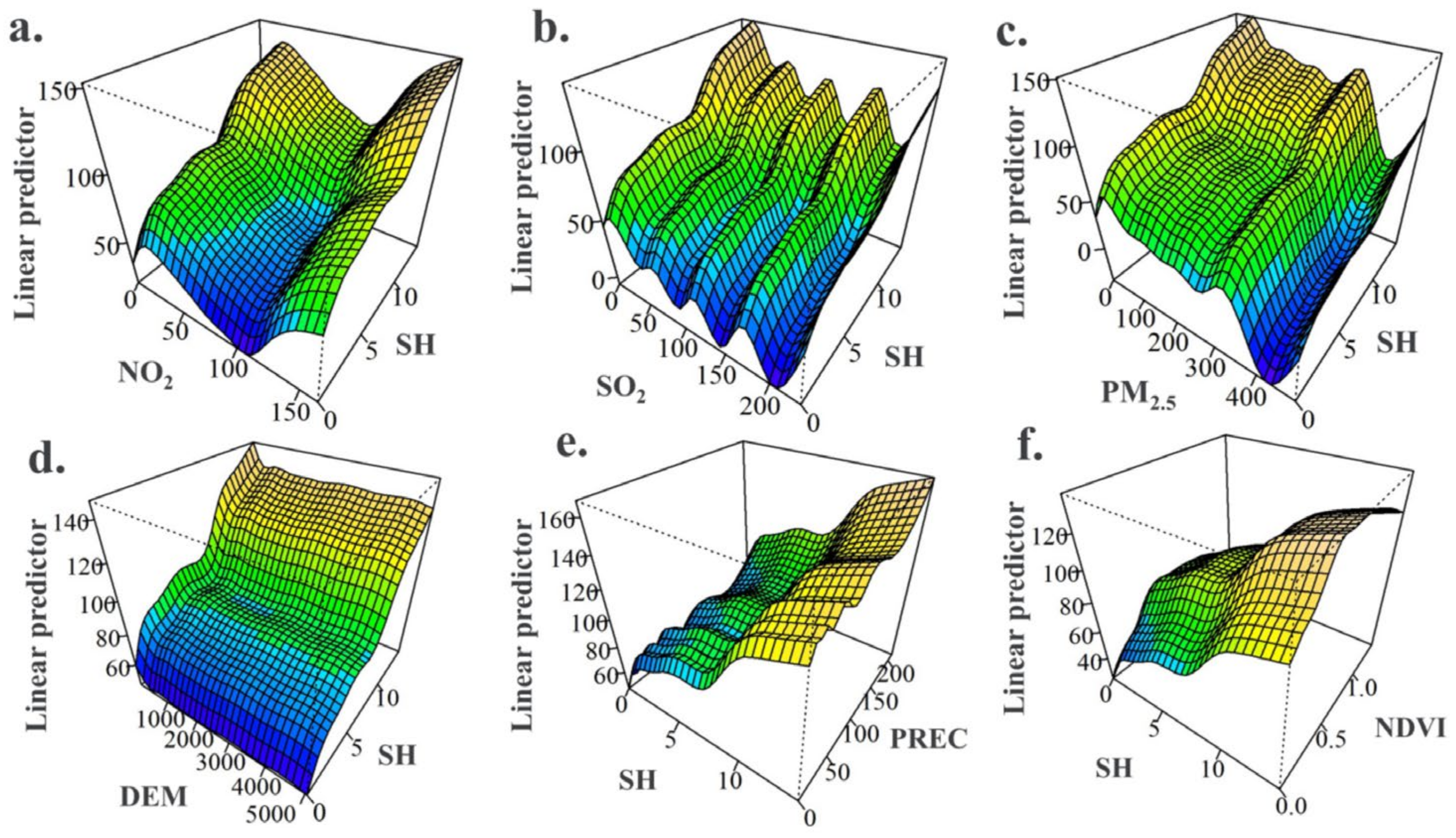
3.5. Interaction of Different Factors on the Variation of Urban O₃ Concentration

The variation of urban O₃ concentration was the result of the compound action of multiple factors, rather than a simple single factor control [57]. To further explore the main driving factors of atmospheric pollutants and meteorological factors on the variation of urban ozone concentration on the Chinese mainland, NO₂, SO₂, PM_2.5, DEM, SH, PREC and NDVI were selected as explanatory variables, and a GAM model under the interaction of multiple factors was constructed. Through pairwise combination, 21 groups of interaction terms were obtained. The results showed that these 21 groups of results all passed the significance test, and the effect on the change of ozone concentration was significant at the level of p < 0.01 (Table S5). In the model (GAM), the adjusted R² was 0.609, and the maximum variance explanation rate was 60.9%, indicating that each interaction term has a good explanation degree for O₃ concentration, and the model fitting effect reached the standard. In addition, the interaction F value of SH and PREC (5988.0), SH and NO₂ (5673.7), SH and DEM (5567.8), SH and SO₂ (5522.0), SH and PM_2.5 (5462.2) was higher than that of other factors, and the interaction between SH and other factors significantly affected the variation of O₃ concentration. Numerous studies have confirmed the significant contribution of sunshine hours to urban O₃ concentration, mainly because sunshine hours affected the intensity of solar radiation (ultraviolet light) and the temperature of photochemical reactions [57,58]. However, the interaction of sunshine hours and other factors on the change of O₃ requires further detailed analysis.

The interaction between SH and NO₂, SH and SO₂, SH and DEM, SH and PREC, SH and NDVI all showed stimulating effects on the increase of O₃ concentration (Figure 7a–f). This result indicated that the risk of urban ozone pollution was exacerbated by unfavorable conditions of both pollutants and meteorological elements in areas with strong solar radiation. In general, when the concentration of NO₂ was below 100 μg/m³, the response of O₃ concentration to the interaction of NO₂ and other factors was not obvious. However, when the NO₂ concentration exceeded the threshold (100 μg/m³), the O₃ concentration showed a rapid increase as the concentration of NO_2, and other pollutants increased (Figure S6a–c). PM_2.5 concentrations showed different characteristics from other atmospheric pollutants. With the increase of PM_2.5 concentration, the positive promotion effect of other factors on O₃ was shielded (Figure S5f,j–l). Some studies have confirmed that the O₃ pollution season has been extended from winter to spring under the background of reduced PM_2.5 and NO_x concentrations in the North China Plain [37]. However, it can be seen from the interaction relationship between PM_2.5 and other factors that reducing the emission of PM_2.5 containing sulfate, nitrate and organic components could significantly reduce the O₃ concentration. The role of precipitation was similar to that of PM_2.5, with high-intensity precipitation attenuating the contribution of other factors (Figure S6d,h,k,m), but high-intensity precipitation and prolonged sunshine promoted the production of O₃ (Figure 7e). When NDVI was lower than ~0.5, with the increase of NDVI and other pollutant concentrations, the O₃ concentration showed an increasing trend. When NDVI exceeded ~0.5, even if the concentration of other pollutants increased, NDVI suggested the phenomenon of inhibiting the production of O₃ (Figure S6e,i,l,n,o). This is because under low vegetation coverage, the BVOCs released by vegetation can participate in photochemical reactions and promote the generation of O₃, while under high vegetation coverage, the vegetation can block direct sunlight and inhibit the production of photochemical reactions [59,60]. In addition, VOCs (e.g., isoprene) released from plants contribute directly to ground-level O₃ formation, especially under high temperature conditions. VOC emissions increase during warm seasons with high insolation and especially during the flowering periods, often exhibiting exponential temperature dependence [61,62]. Some of the VOCs (e.g., monoterpenes and sesquiterpenes) released by plants can cause an increase in near-surface particulate matter concentrations [63,64]. However, the transfer of VOCs between the gas and solid phases can slow or exacerbate the formation of urban O₃ [61]. Under high temperature conditions, VOCs released by plants can promote the formation of O₃ in cities. However, plants can also prevent the formation of O₃ through surface adsorption and the weakening of light intensity. These two opposite behaviors have significant changes in different regions and times.

4. Conclusions

This study explored the spatial clustering and temporal dynamic evolution characteristics of the O₃ concentration in cities from mainland China on a long-term scale. The different effects of topography and vegetation characteristics on the distribution of O₃ in various regions of China were also verified. The results suggested that the O₃ concentration in China’s cities showed an upward trend from 2015 to 2018, followed by a downward trend after 2018. The variations in the O₃ concentration had obvious seasonal characteristics (summer > spring > autumn > winter), where the change of the O₃ concentration in May should be the focus of attention. From 2015 to 2016, the urban O₃ concentration pollution area exhibited a spot-like distribution mainly concentrated in the Beijing-Tianjin-Hebei region, the Shandong Peninsula, and the Yangtze River Delta region. However, by 2018, the polluted area expanded from spots to surface. The areas of high O₃ concentration included most cities in North China, East China, and Central China, and even some cities in Southwest China were also polluted by O₃. On the national scale, the distribution of O₃ had the characteristics of spatial dependence and aggregation. On a regional scale, the O₃ distribution areas of high concentration were mainly concentrated in Beijing-Tianjin-Hebei, Shandong, Jiangsu, Henan, and other regions. In addition, the standard deviation ellipse of the urban O₃ concentration covered the entire eastern part of mainland China. Overall, the mean center of the standard deviation ellipse tended to move to the south with the time variation. DEM had a significant positive correlation with the O₃ concentration in Southwest and Northwest China. Vegetation removed air pollutants by preventing the migration and diffusion of atmospheric particles and plant transpiration, especially in Southwest China, Northwest China, and Central China, where the suppression effect of vegetation on local O₃ was more obvious than that in other regions.

References

1. Derwent, R.G.; Jenkin, M.E.; Saunders, S.M. Photochemical ozone creation potentials for a large number of reactive hydrocarbons under European conditions. Atmos. Environ. 1996, 30, 181–199. [Google Scholar] [CrossRef]
2. Richter, A.; Burrows, J.P.; Nuss, H.; Granier, C.; Niemeier, U. Increase in tropospheric nitrogen dioxide over China observed from space. Nature 2005, 437, 129–132. [Google Scholar] [CrossRef] [PubMed]
3. Huffman, L.J.; Judy, D.J.; Brumbaugh, K.; Frazer, D.G.; Reynolds, J.S.; McKinney, W.G.; Goldsmith, W.T. Hyperthyroidism increases the risk of ozone-induced lung toxicity in rats. Toxicol. Appl. Pharmacol. 2001, 173, 18–26. [Google Scholar] [CrossRef] [PubMed]
4. Khatri, S.B.; Holguin, F.C.; Ryan, P.B.; Mannino, D.; Erzurum, S.C.; Teague, W.G. Association of ambient ozone exposure with airway inflammation and allergy in adults with Asthma. J. Asthma. 2009, 46, 777–785. [Google Scholar] [CrossRef]
5. Li, J.; Huang, J.; Cao, R.; Yin, P.; Wang, L.J.; Liu, Y.; Pan, X.C.; Li, G.X.; Zhou, M.G. The association between ozone and years of life lost from stroke, 2013–2017: A retrospective regression analysis in 48 major Chinese cities. J. Hazard. Mater. 2021, 405, 124220. [Google Scholar] [CrossRef]
6. Fuller, C.H.; Jones, J.W.; Roblin, D.W. Evaluating changes in ambient ozone and respiratory-related healthcare utilization in the Washington, DC metropolitan area. Environ. Res. 2020, 186, 109603. [Google Scholar] [CrossRef]
7. Debaje, S.B. Estimated crop yield losses due to surface ozone exposure and economic damage in India. Environ. Sci. Pollut. Res. 2014, 21, 7329–7338. [Google Scholar] [CrossRef] [Green Version]
8. Fine, R.; Miller, M.B.; Burley, J.; Jaffe, D.A.; Pierce, R.B.; Lin, M.Y.; Gustin, M.S. Variability and sources of surface ozone at rural sites in Nevada, USA: Results from two years of the Nevada Rural Ozone Initiative. Sci. Total Environ. 2015, 530, 471–482. [Google Scholar] [CrossRef]
9. He, G.W.; Deng, T.; Wu, D.; Wu, C.; Huang, X.F.; Li, Z.N.; Yin, C.Q.; Zou, Y.; Song, L.; Ouyang, S.S.; et al. Characteristics of boundary layer ozone and its effect on surface ozone concentration in Shenzhen, China: A case study. Sci. Total Environ. 2021, 791, 148044. [Google Scholar] [CrossRef]
10. Shu, L.; Wang, T.J.; Han, H.; Xie, M.; Chen, P.L.; Li, M.M.; Wu, H. Summertime ozone pollution in the Yangtze River Delta of eastern China during 2013–2017: Synoptic impacts and source apportionment. Environ. Pollut. 2020, 257, 113631. [Google Scholar] [CrossRef]
11. Deng, C.X.; Tian, S.; Li, Z.W.; Li, K. Spatiotemporal characteristics of PM2.5 and ozone concentrations in Chinese urban clusters. Chemosphere 2022, 295, 133813. [Google Scholar] [CrossRef]
12. Fang, X.Z.; Xiao, H.Y.; Sun, H.X.; Liu, C.; Zhang, Z.Y.; Xie, Y.J.; Liang, Y.; Wang, F. Characteristics of ground-Level ozone from 2015 to 2018 in BTH Area, China. Atmosphere 2020, 11, 130. [Google Scholar] [CrossRef] [Green Version]
13. Liu, H.L.; Zhang, M.G.; Han, X. A review of surface ozone source apportionment in China. Atmos. Ocean Sci. Lett. 2020, 13, 470–484. [Google Scholar] [CrossRef]
14. Ou, J.M.; Huang, Z.J.; Klimont, Z.; Jia, G.L.; Zhang, S.H.; Li, C.; Meng, J.; Mi, Z.F.; Zheng, H.R.; Shan, Y.L.; et al. Role of export industries on ozone pollution and its precursors in China. Nat. Commun. 2020, 11, 5492. [Google Scholar] [CrossRef]
15. Feng, T.; Bei, N.F.; Zhao, S.Y.; Wu, J.R.; Liu, S.X.; Li, X.; Liu, L.; Wang, R.N.; Zhang, X.; Tie, X.X.; et al. Nitrate debuts as a dominant contributor to particulate pollution in Beijing: Roles of enhanced atmospheric oxidizing capacity and decreased sulfur dioxide emission. Atmos. Environ. 2021, 244, 117995. [Google Scholar] [CrossRef]
16. Gao, C.; Xiu, A.J.; Zhang, X.L.; Chen, W.W.; Liu, Y.; Zhao, H.M.; Zhang, S.C. Spatiotemporal characteristics of ozone pollution and policy implications in Northeast China. Atmos. Pollut. Res. 2020, 11, 357–369. [Google Scholar] [CrossRef]
17. Xu, J.W.; Huang, X.; Wang, N.; Li, Y.Y.; Ding, A.J. Understanding ozone pollution in the Yangtze River Delta of eastern China from the perspective of diurnal cycles. Sci. Total Environ. 2021, 752, 141928. [Google Scholar] [CrossRef]
18. Rufeger, W.; Mieth, P. The DYMOS system and its application to urban areas. Environ. Model. Softw. 1998, 13, 287–294. [Google Scholar] [CrossRef]
19. Liu, B.S.; Liang, D.N.; Yang, J.M.; Dai, Q.L.; Bi, X.H.; Feng, Y.C.; Yuan, J.; Xiao, Z.M.; Zhang, Y.F.; Xu, H. Characterization and source apportionment of volatile organic compounds based on 1-year of observational data in Tianjin, China. Environ. Pollut. 2016, 218, 757–769. [Google Scholar] [CrossRef]
20. Zhang, J.; Wang, C.; Qu, K.; Ding, J.W.; Shang, Y.Q.; Liu, H.F.; Wei, M. Characteristics of ozone pollution, regional distribution and causes during 2014–2018 in Shandong Province, East China. Atmosphere 2019, 10, 509. [Google Scholar] [CrossRef] [Green Version]
21. Zhu, B.; Kang, H.Q.; Zhu, T.; Su, J.F.; Hou, X.W.; Gao, J.H. Impact of Shanghai urban land surface forcing on downstream city ozone chemistry. J. Geophys. Res. Atmos. 2015, 120, 4340–4351. [Google Scholar] [CrossRef]
22. Zhu, K.G.; Xie, M.; Wang, T.J.; Cai, J.X.; Li, S.B.; Feng, W. A modeling study on the effect of urban land surface forcing to regional meteorology and air quality over South China. Atmos. Environ. 2017, 152, 389–404. [Google Scholar] [CrossRef]
23. Chen, Z.Y.; Zhuang, Y.; Xie, X.M.; Chen, D.L.; Cheng, N.L.; Yang, L.; Li, R.Y. Understanding long-term variations of meteorological influences on ground ozone concentrations in Beijing During 2006–2016. Environ. Pollut. 2019, 245, 29–37. [Google Scholar] [CrossRef] [PubMed]
24. Li, X.L.; Hu, X.M.; Shi, S.Y.; Shen, L.D.; Luan, L.; Ma, Y.J. Spatiotemporal variations and regional transport of air pollutants in two urban agglomerations in Northeast China Plain. Chin. Geogr. Sci. 2019, 29, 917–933. [Google Scholar] [CrossRef] [Green Version]
25. Wang, Z.B.; Li, J.X.; Liang, L.W. Spatio-temporal evolution of ozone pollution and its influencing factors in the Beijing-Tianjin-Hebei Urban Agglomeration. Environ. Pollut. 2020, 256, 113419. [Google Scholar] [CrossRef]
26. He, J.J.; Gong, S.L.; Yu, Y.; Yu, L.J.; Wu, L.; Mao, H.J.; Song, C.B.; Zhao, S.P.; Liu, H.L.; Li, X.Y.; et al. Air pollution characteristics and their relation to meteorological conditions during 2014–2015 in major Chinese cities. Environ. Pollut. 2017, 223, 484–496. [Google Scholar] [CrossRef]
27. Ma, T.; Duan, F.K.; He, K.B.; Qin, Y.; Tong, D.; Geng, G.N.; Liu, X.Y.; Li, H.; Yang, S.; Ye, S.Q.; et al. Air pollution characteristics and their relationship with emissions and meteorology in the Yangtze River Delta region during 2014–2016. J. Environ. Sci. 2019, 83, 8–20. [Google Scholar] [CrossRef]
28. Guo, B.; Wang, X.; Pei, L.; Su, Y.; Zhang, D.; Wang, Y. Identifying the spatiotemporal dynamic of PM2.5 concentrations at multiple scales using geographically and temporally weighted regression model across China during 2015–2018. Sci. Total Environ. 2021, 751, 141765. [Google Scholar] [CrossRef]
29. Harris, P.; Brunsdon, C.; Fotheringham, A.S. Links, comparisons and extensions of the geographically weighted regression model when used as a spatial predictor. Stoch. Environ. Res. Risk Assess. 2011, 25, 123–138. [Google Scholar] [CrossRef] [Green Version]
30. Ma, Y.X.; Ma, B.J.; Jiao, H.R.; Zhang, Y.F.; Xin, J.Y.; Yu, Z. An analysis of the effects of weather and air pollution on tropospheric ozone using a generalized additive model in Western China: Lanzhou, Gansu. Atmos. Environ. 2020, 224, 117342. [Google Scholar] [CrossRef]
31. Chu, H.J.; Lin, C.Y.; Liau, C.J.; Kuo, Y.M. Identifying controlling factors of ground-level ozone levels over southwestern Taiwan using a decision tree. Atmos. Environ. 2012, 60, 142–152. [Google Scholar] [CrossRef]
32. Jiang, Z.J.; Li, J.; Lu, X.; Gong, C.; Zhang, L.; Liao, H. Impact of western Pacific subtropical high on ozone pollution over eastern China. Atmos. Chem. Phys. 2021, 21, 2601–2613. [Google Scholar] [CrossRef]
33. Li, K.; Jacob, D.J.; Liao, H.; Qiu, Y.L.; Shen, L.; Zhai, S.X.; Bates, K.H.; Sulprizio, M.P.; Song, S.J.; Lu, X.; et al. Ozone pollution in the North China Plain spreading into the late-winter haze season. Proc. Natl. Acad. Sci. USA 2021, 118, e2015797118. [Google Scholar] [CrossRef]
34. Zhou, Z.H.; Tan, Q.W.; Deng, Y.; Lu, C.W.; Song, D.L.; Zhou, X.L.; Zhang, X.; Jiang, X. Source profiles and reactivity of volatile organic compounds from anthropogenic sources of a megacity in southwest China. Sci. Total Environ. 2021, 790, 148149. [Google Scholar] [CrossRef]
35. Yang, J.; Sun, J.; Ge, Q.S.; Li, X.M. Assessing the impacts of urbanization-associated green space on urban land surface temperature: A case study of Dalian, China. Urban For. Urban Greening. 2017, 22, 1–10. [Google Scholar] [CrossRef]
36. Yamaji, K.; Ohara, T.; Uno, I.; Tanimoto, H.; Kurokawa, J.; Akimoto, H. Analysis of the seasonal variation of ozone in the boundary layer in East Asia using the Community Multi-scale Air Quality model: What controls surface ozone levels over Japan? Atmos. Environ. 2006, 40, 1856–1868. [Google Scholar] [CrossRef]
37. Li, R.; Cui, L.L.; Li, J.L.; Zhao, A.; Fu, H.B.; Wu, Y.; Zhang, L.W.; Kong, L.D.; Chen, J.M. Spatial and temporal variation of particulate matter and gaseous pollutants in China during 2014–2016. Atmos. Environ. 2017, 161, 235–246. [Google Scholar] [CrossRef]
38. Ou, J.M.; Zheng, J.Y.; Li, R.R.; Huang, X.B.; Zhong, Z.M.; Zhong, L.J.; Lin, H. Speciated OVOC and VOC emission inventories and their implications for reactivity-based ozone control strategy in the Pearl River Delta region, China. Sci. Total Environ. 2015, 530, 393–402. [Google Scholar] [CrossRef]
39. Yao, Y.R.; Wang, W.; Ma, K.; Tan, H.R.; Zhang, Y.; Fang, F.M.; He, C. Transmission paths and source areas of near-surface ozone pollution in the Yangtze River delta region, China from 2015 to 2021. J. Environ. Manag. 2023, 330, 117105. [Google Scholar] [CrossRef]
40. Li, K.; Jacob, D.J.; Liao, H.; Shen, L.; Zhang, Q.; Bates, K.H. Anthropogenic drivers of 2013–2017 trends in summer surface ozone in China. Proc. Natl. Acad. Sci. USA 2019, 116, 422–427. [Google Scholar] [CrossRef] [Green Version]
41. Chen, Z.Y.; Li, R.Y.; Chen, D.L.; Zhuang, Y.; Gao, B.B.; Yang, L.; Li, M.C. Understanding the causal influence of major meteorological factors on ground ozone concentrations across China. J. Clean. Prod. 2020, 242, 118498. [Google Scholar] [CrossRef]
42. Kang, M.J.; Zhang, J.; Zhang, H.L.; Ying, Q. On the Relevancy of observed ozone increase during COVID-19 lockdown to summertime ozone and PM2.5 control policies in China. Environ. Sci. Technol. Lett. 2021, 8, 289–294. [Google Scholar] [CrossRef]
43. Wan, S.; Cui, K.P.; Wang, Y.F.; Wu, J.L.; Huang, W.S.; Xu, K.J.; Zhang, J.J. Impact of the COVID-19 event on trip intensity and air quality in Southern China. Aerosol Air Qual. Res. 2020, 20, 1727–1747. [Google Scholar] [CrossRef]
44. Yang, G.F.; Liu, Y.H.; Li, X.N. Spatiotemporal distribution of ground-level ozone in China at a city level. Sci. Rep. 2020, 10, 7229. [Google Scholar] [CrossRef] [PubMed]
45. Lou, S.J.; Liao, H.; Yang, Y.; Mu, Q. Simulation of the interannual variations of tropospheric ozone over China: Roles of variations in meteorological parameters and anthropogenic emissions. Atmos. Environ. 2016, 122, 839–851. [Google Scholar] [CrossRef]
46. Xu, J.L.; Zhu, Y.X. Effects of the meteorological factors on the ozone pollution near the ground. Chin. J. Atmosph. Sci. 1994, 18, 751–757. [Google Scholar]
47. Lin, M.Y.; Horowitz, L.W.; Xie, Y.Y.; Paulot, F.; Malyshev, S.; Shevliakova, E.; Finco, A.; Gerosa, G.; Kubistin, D.; Pilegaard, K. Vegetation feedbacks during drought exacerbate ozone air pollution extremes in Europe. Nat. Clim. Change 2020, 10, 444–451. [Google Scholar] [CrossRef]
48. Fan, Z.Y.; Zhan, Q.M.; Yang, C.; Liu, H.M.; Zhan, M. How did distribution patterns of aarticulate matter air pollution (PM(2.5) and PM10) change in China during the COVID-19 outbreak: A spatiotemporal investigation at Chinese City-Level. Int. J. Environ. Res. Public Health 2020, 17, 6274. [Google Scholar] [CrossRef]
49. Fotheringham, A.S.; Yue, H.; Li, Z.Q. Examining the influences of air quality in China’s cities using multi-scale geographically weighted regression. Trans. GIS. 2019, 23, 1444–1464. [Google Scholar] [CrossRef]
50. Sillman, S. The use of NOy, H2O2, and HNO3 as indicators for ozone-NOx-hydrocarbon sensitivity in urban locations. J. Geophys. Res. Atmos. 1995, 100, 14175–14188. [Google Scholar] [CrossRef]
51. Turnock, S.T.; Mann, G.W.; Woodhouse, M.T.; Dalvi, M.; O’Connor, F.M.; Carslaw, K.S.; Spracklen, D.V. The impact of changes in cloud water pH on aerosol radiative forcing. Geophys. Res. Lett. 2019, 46, 4039–4048. [Google Scholar] [CrossRef] [Green Version]
52. Cui, H.Y.; Chen, W.H.; Dai, W.; Liu, H.; Wang, X.M.; He, K.B. Source apportionment of PM2.5 in Guangzhou combining observation data analysis and chemical transport model simulation. Atmos. Environ. 2015, 116, 262–271. [Google Scholar] [CrossRef]
53. Susaya, J.; Kim, K.H.; Shon, Z.H.; Brown, R.J.C. Demonstration of long-term increases in tropospheric O3 levels: Causes and potential impacts. Chemosphere 2013, 92, 1520–1528. [Google Scholar] [CrossRef]
54. Wang, T.; Xue, L.K.; Brimblecombe, P.; Lam, Y.F.; Li, L.; Zhang, L. Ozone pollution in China: A review of concentrations, meteorological influences, chemical precursors, and effects. Sci. Total Environ. 2017, 575, 1582–1596. [Google Scholar] [CrossRef]
55. Min, R.Q.; Wang, F.; Wang, Y.B.; Song, G.X.; Zheng, H.; Zhang, H.P.; Ru, X.T.; Song, H.Q. Contribution of local and surrounding area anthropogenic emissions to a high ozone episode in Zhengzhou, China. Environ. Res. 2022, 212, 113440. [Google Scholar] [CrossRef]
56. Toh, Y.Y.; Lim, S.F.; von Glasow, R. The influence of meteorological factors and biomass burning on surface ozone concentrations at Tanah Rata, Malaysia. Atmos. Environ. 2013, 70, 435–446. [Google Scholar] [CrossRef]
57. Hu, C.Y.; Kang, P.; Jaffe, D.A.; Li, C.K.; Zhang, X.L.; Wu, K.; Zhou, M.W. Understanding the impact of meteorology on ozone in 334 cities of China. Atmos. Environ. 2021, 248, 118221. [Google Scholar] [CrossRef]
58. Bai, J.H. Analysis of ultraviolet radiation in clear skies in Beijing and its affecting factors. Atmos. Environ. 2011, 45, 6930–6937. [Google Scholar] [CrossRef]
59. Youn, J.S.; Wang, Z.; Wonaschutz, A.; Arellano, A.; Betterton, E.A.; Sorooshian, A. Evidence of aqueous secondary organic aerosol formation from biogenic emissions in the North American Sonoran Desert. Geophys. Res. Lett. 2013, 40, 3468–3472. [Google Scholar] [CrossRef] [Green Version]
60. Richards, D.R.; Edwards, P.J. Quantifying street tree regulating ecosystem services using Google Street View. Ecol. Indic. 2017, 77, 31–40. [Google Scholar] [CrossRef]
61. Churkina, G.; Kuik, F.; Bonn, B.; Lauer, A.; Grote, R.; Tomiak, K.; Butler, T.M. Effect of VOC Emissions from Vegetation on Air Quality in Berlin during a Heatwave. Environ. Sci. Technol. 2017, 51, 6120–6130. [Google Scholar] [CrossRef] [PubMed]
62. Guenther, A.B.; Zimmerman, P.R.; Harley, P.C.; Monson, R.K.; Fall, R. Isoprene and monoterpene emission rate variability: Model evaluations and sensitivity analyses. J. Geophys. Res. 1993, 98, 12609–12617. [Google Scholar] [CrossRef] [Green Version]
63. Chameides, W.; Lindsay, R.; Richardson, J.; Kiang, C. The role of biogenic hydrocarbons in urban photochemical smog: Atlanta as a case study. Science 1988, 241, 1473–1475. [Google Scholar] [CrossRef] [PubMed]
64. Hoffmann, T.; Odum, J.; Bowman, F.; Collins, D.; Klockow, D.; Flagan, R.; Seinfeld, J. Formation of Organic Aerosols from the Oxidation of Biogenic Hydrocarbons. J. Atmos. Chem. 1997, 26, 189–222. [Google Scholar] [CrossRef]
65. Anand, V.; Panicker, A.S.; Beig, G. Gaseous pollutants over different sites in a metropolitan region (Pune) over India. SN Appl. Sci. 2020, 2, 682. [Google Scholar] [CrossRef] [Green Version]
66. Andreev, V.V.; Arshinov, M.Y.; Belan, B.D.; Davydov, D.K.; Elansky, N.F.; Zhamsueva, G.S.; Zayakhanov, A.S.; Ivlev, G.A.; Kozlov, A.V.; Kotel’nikov, S.N.; et al. Surface Ozone Concentration over Russian Territory in the First Half of 2020. Atmos. Ocean. Opt. 2020, 33, 671–681. [Google Scholar] [CrossRef]
67. Ezimand, K.; Kakroodi, A.A. Prediction and Spatio–Temporal analysis of ozone concentration in a metropolitan area. Ecol. Indic. 2019, 103, 589–598. [Google Scholar] [CrossRef]
68. Kobza, J.; Geremek, M.; Dul, L. Ozone Concentration Levels in Urban Environments-Upper Silesia Region Case Study. Int. J. Environ. Res. Public Health 2021, 18, 1473. [Google Scholar] [CrossRef]
69. Krug, A.; Fenner, D.; Mucke, H.G.; Scherer, D. The contribution of air temperature and ozone to mortality rates during hot weather episodes in eight German cities during the years 2000 and 2017. Nat. Hazards Earth Syst. Sci. 2020, 20, 3083–3097. [Google Scholar] [CrossRef]
70. Sicard, P.; Serra, R.; Rossello, P. Spatiotemporal trends in ground-level ozone concentrations and metrics in France over the time period 1999–2012. Environ. Res. 2016, 149, 122–144. [Google Scholar] [CrossRef]
Figure 1. The heat map of urban O3 concentration (MDA8) in mainland China from the year of 2015 to 2020. (The “grey” colour in Figure 1 represents the days when there were less than 14 valid MDA8 data and the MDA8 value did not exceed the limit value criteria between 08:00 and 24:00. Missing dates are 22–26 December 2018).
Ijerph 20 03810 g001
Figure 2. Trend surface analysis of the urban O3 concentration (the 90th percentile of MDA8) in mainland China from 2015 to 2020.
Ijerph 20 03810 g002
Figure 3. The spatial distribution of the urban O3 concentration (the 90th percentile of MDA8) in the mainland of China from the years 2015 to 2020. (a) 2015; (b) 2016; (c) 2017; (d) 2018; (e) 2019; (f) 2020. (Note: Urban O3 concentrations are derived from the average values of the effective monitoring stations in each city).
Ijerph 20 03810 g003
Figure 4. The spatial clustering pattern of the urban O3 concentration in mainland China from 2015 to 2020. (a) 2015; (b) 2016; (c) 2017; (d) 2018; (e) 2019; (f) 2020. (Note: Urban O3 concentrations are derived from the average values of the effective monitoring stations in each city).
Ijerph 20 03810 g004
Figure 5. Time series of the mean center and standard deviational ellipse of the O3 concentration in mainland China in 2015–2020. (Note: Urban O3 concentrations are derived from the average values of the effective monitoring stations in each city).
Ijerph 20 03810 g005
Figure 6. Spatial patterns of coefficients in the MGWR. (a) Intercept, (b) NO2, (c) SO2, (d) PM2.5, (e) DEM, (f) sunshine hours, (g) precipitation, (h) NDVI.
Ijerph 20 03810 g006
Figure 7. Interaction of different factors on the variation of urban O3 concentration Three-dimensional effect plots. (a) NO2 and sunshine hours (SH); (b) SO2 and sunshine hours (SH); (c) PM2.5 and sunshine hours (SH); (d) Digital Elevation Model (DEM) and sunshine hours (SH); (e) precipitation (PREC) and sunshine hours (SH); (f) normalized difference vegetation index (NDVI) and sunshine hours (SH).
Ijerph 20 03810 g007