

A Study of Urban Haze and Its Association with Cold Surge and Sea Breeze for Greater Bangkok

 , ,
, ,
Abstract
:1. Introduction
2. Data and Methods
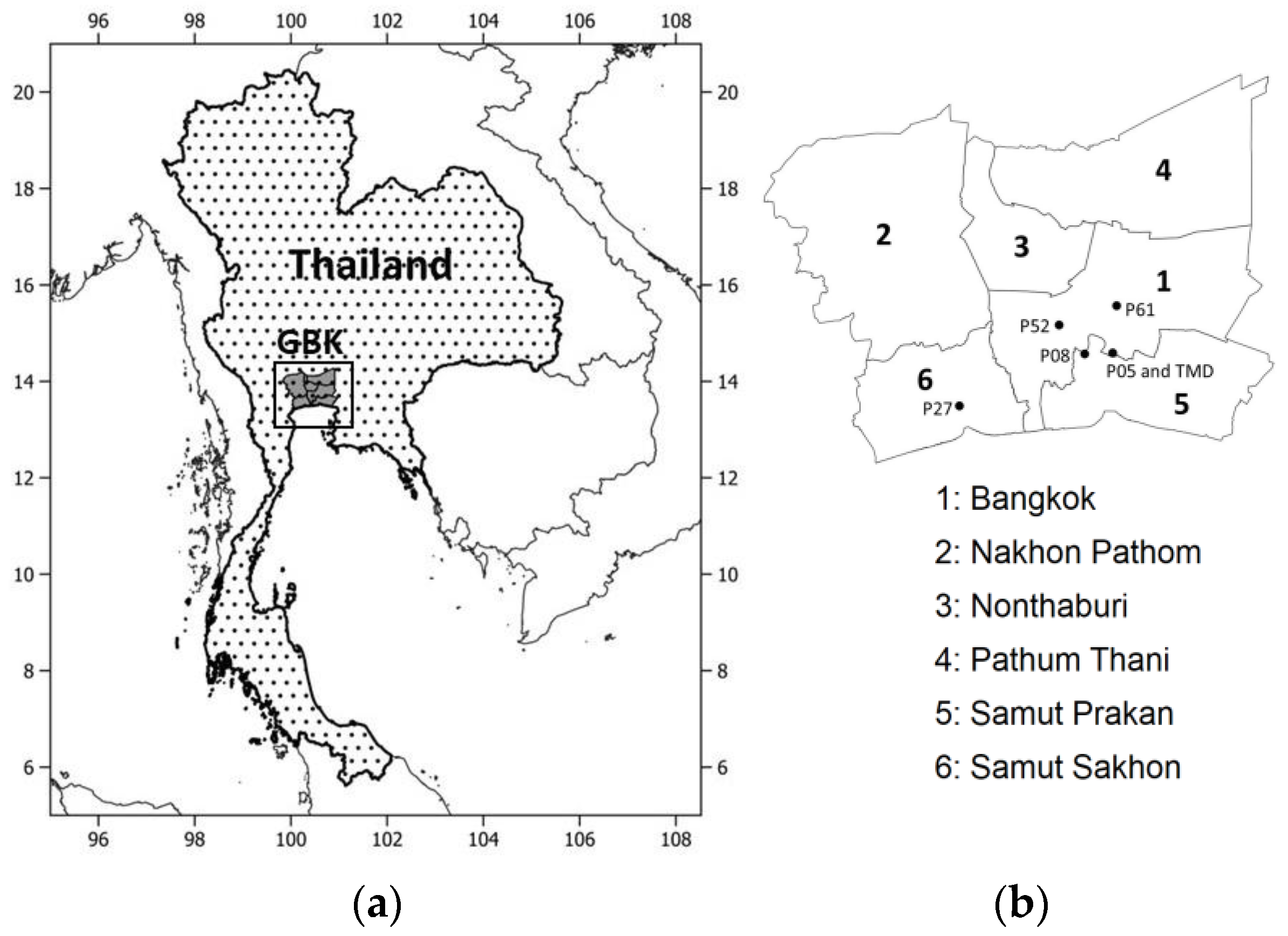
2.1. Study Area
2.2. Data
2.3. Haze Days and Episodes
2.4. Cold Surge Identification
2.5. Sea Breeze Identification
2.6. Biomass Burning and Back-Trajectories
2.7. Identification of Different Haze Types
- (a)
- Type I: Haze episodes are associated with the arrival of cold surges in GBK during the pre-haze period, which brings cool and relatively strong winds. After a few days of its arrival, it creates stagnant air conditions with limited vertical motion and calm winds. These conditions suppress the vertical dilution of air pollutants and are also not transported horizontally, leading to the accumulation of air pollutants and hence the haze conditions. In short, Type I corresponds to “cold-surge influenced”.
- (b)
- Type II: Haze episodes tend to be under the influence of sea breezes from the Gulf of Thailand for most of the days. This category represents haze episodes that are induced by the combined effect of (1) the recirculation of air pollutants by sea breezes, which brings them back to the city after being initially transported away from the city, (2) potentially developed thermal internal boundary layer due to the advection of cool and stable air over the hot land surface. Air is thermally unstable near the Earth’s surface below cool and stable air, which acts as a cap and prevents the vertical mixing of air pollutants. In short, Type II corresponds to “sea-breeze influenced”.
- (c)
- Type III: Haze episodes are synergistically influenced by the cold surge and sea breeze. A typical haze episode is triggered by the arrival of cold surges in the pre-haze period as suggested for Type I, but as cold surges dissipate, the sea breeze starts, which could potentially affect air pollution dispersion as mentioned in Type II. In some episodes, reverse patterns were also observed when SB days were identified for the first few days followed by CS days.
- (d)
- Type IV: Haze episodes are not affected by either cold surges or sea breeze. Most of the haze episodes are short 1-day episodes and are also affected by biomass burning.
2.8. Effect of Secondary Aerosols
3. Results
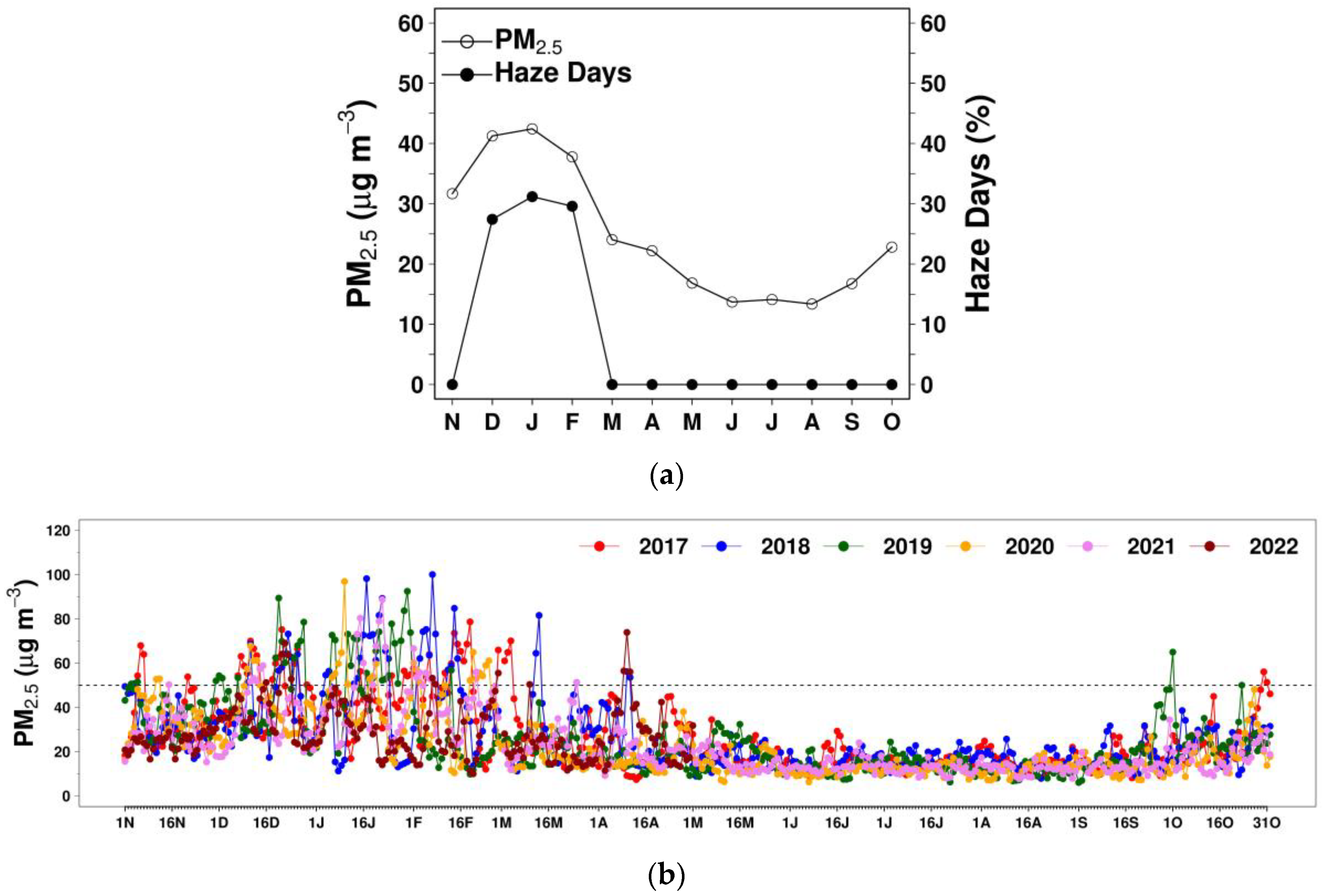
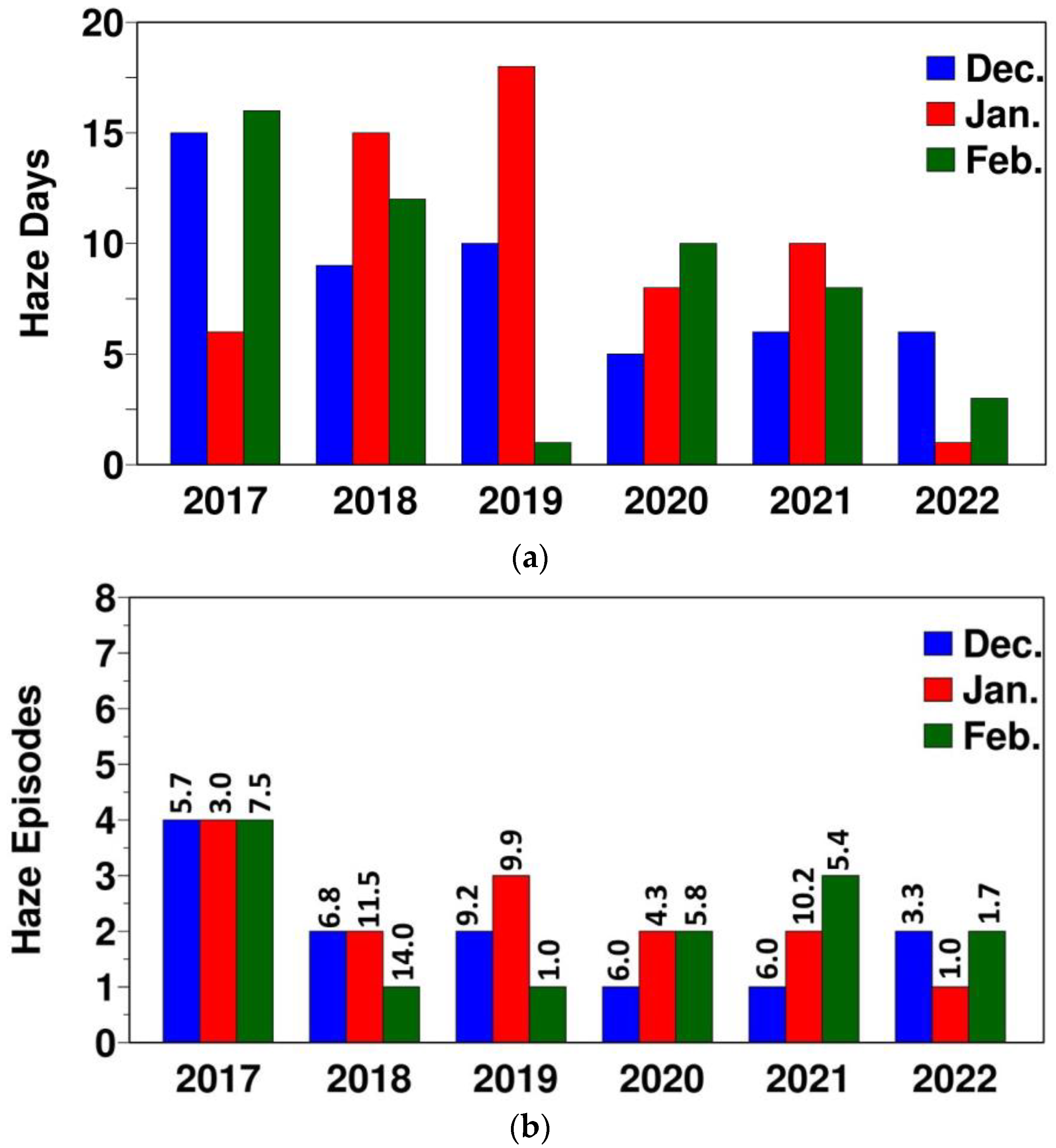
3.1. Temporal Characteristics of Identified Haze Days and Haze Episodes
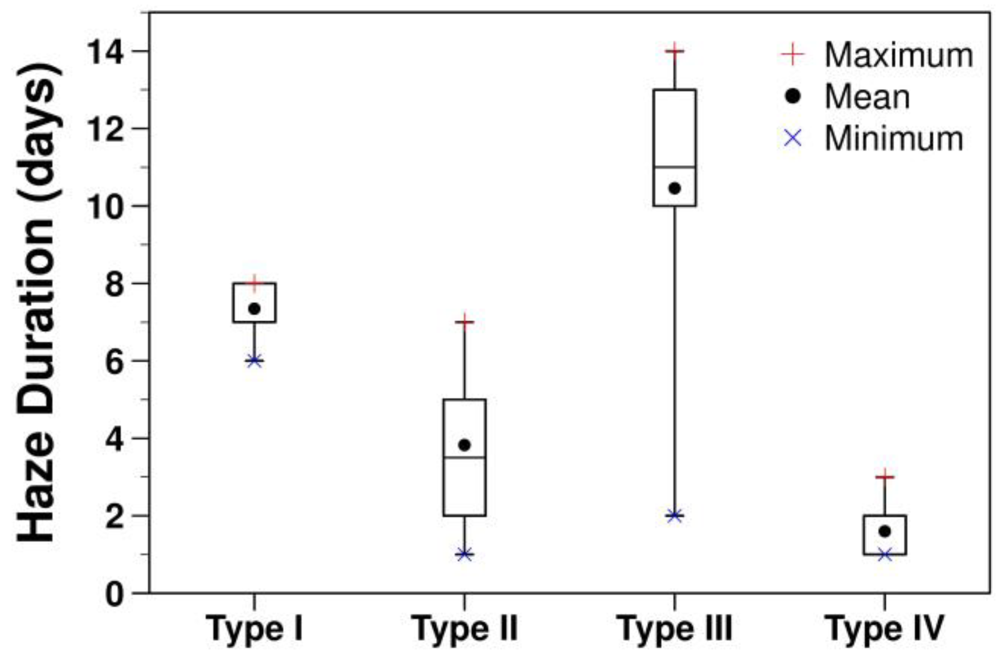
3.2. Characteristics of Different Haze Types
- (a)
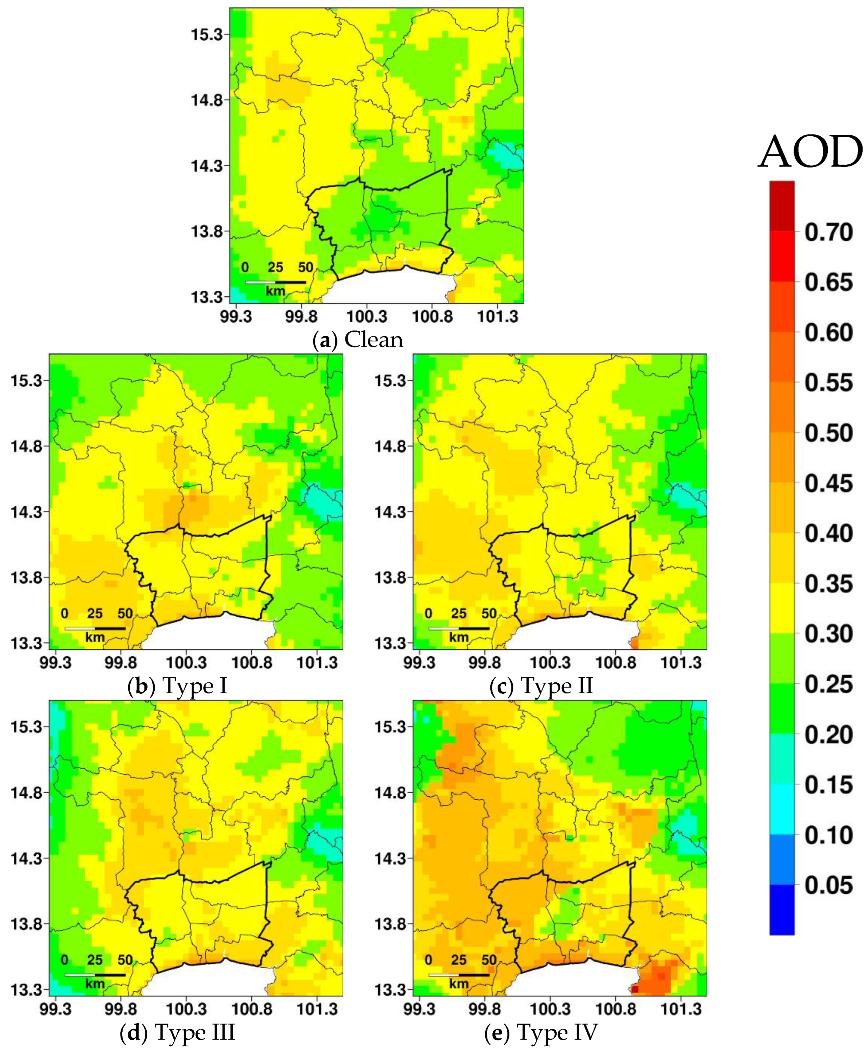
- Type I: Four haze episodes are categorized in this haze type. This is the second most persistent haze type, and the average duration of haze episodes is 7.3 days. It has two haze episodes of eight days and a haze episode each of six and seven days, respectively (Table 2). In terms of particulate pollution, this is the second most polluted haze type with an average PM2.5 of 58.5 μg m−3. As this haze type is triggered by the cold surge over Greater Bangkok, which brings cold and dry air, it has the lowest average temperature and average relative humidity (26.9 °C and 49.1%, respectively). A cold surge generally induces less cloud cover, which leads to an increase in global radiation as shown by the lowest average cloud cover of 4.9 and the second-highest average global radiation of 456.6 W m−2. Due to more stagnant weather conditions, wind recirculation is relatively low with an average recirculation factor of 0.12. The spatial variation of AOD suggests relatively higher AOD (ranges between 0.2 and 0.6) in Greater Bangkok and connected provinces on the northern and western sides as compared to those on the eastern side and far north. In comparison, AOD over clean days is relatively low over Greater Bangkok.
- (b)
- Type II: This is the most frequent haze type with 15 haze episodes. The average minimum and maximum durations of haze episodes are 3.8 days, 1 day, and 7 days respectively. Nine of the fifteen haze episodes are of only 1–2 days. The average PM2.5 is 56.8 μg m−3. As this haze type is influenced by SB, which brings humid air from the seaside, the highest average RH of 59.1% is reported, while the average temperature is 29.1 °C. The second-lowest average cloud cover and highest average global radiations of 5.1 and 471.1 W m−2, respectively, were reported. Due to the influences of sea breeze, a relatively higher average recirculation factor of 0.3 is found. The average SB duration and SB penetration are 7.6 h and 31.6 km, respectively. Compared with Type I, the aerosol loading is higher at a larger distance from Greater Bangkok and over larger regions, which can be attributed to the advection of air pollutants.
- (c)
- Type III: This is the second most frequent haze type with 11 haze episodes and the most persistent type with an average haze episode duration of 10.5 due to the synergetic effect of the cold surge and sea breeze. This is the most polluted haze type with an average PM2.5 of 62.8 μg m−3. The average values for temperature, relative humidity, cloud cover, global radiation, and recirculation factor are 27.6 °C, 58.1%, 5.2, 453.5 W m−2, and 0.3, respectively. Due to the interaction of the sea breeze with the cold surge from the opposite direction, the average SB duration and SB penetration are lower than those in type II (6.2 h and 20.5 km, respectively). The spread of haze or aerosols is over a larger area in the north, as suggested by higher AOD, which can be attributed to both the advection and dispersion of air pollutants, given multiple persistent haze episodes.
- (d)
- Type IV: This category consists of eight haze episodes, and seven of them are one-day episodes, while the remaining one is a three-day episode. The average PM2.5 under this haze type is 54.1 μg m−3. Many of the haze episodes are associated with biomass burning. The effect of biomass burning on different haze episodes is discussed and illustrated in Section 3.4. The average values for temperature, relative humidity, cloud cover, global radiation, and recirculation factor are 28.4 °C, 58.2%, 5.5, 414.1 W m−2, and 0.2, respectively. The sea breeze was reported on the last day of the 3-day haze episode with duration and penetration of 12 h and 36.2 km, respectively. The spread of aerosol is over larger regions as suggested by higher AOD over the region, which can be attributed to biomass burning.
3.3. Effect of Secondary Aerosols
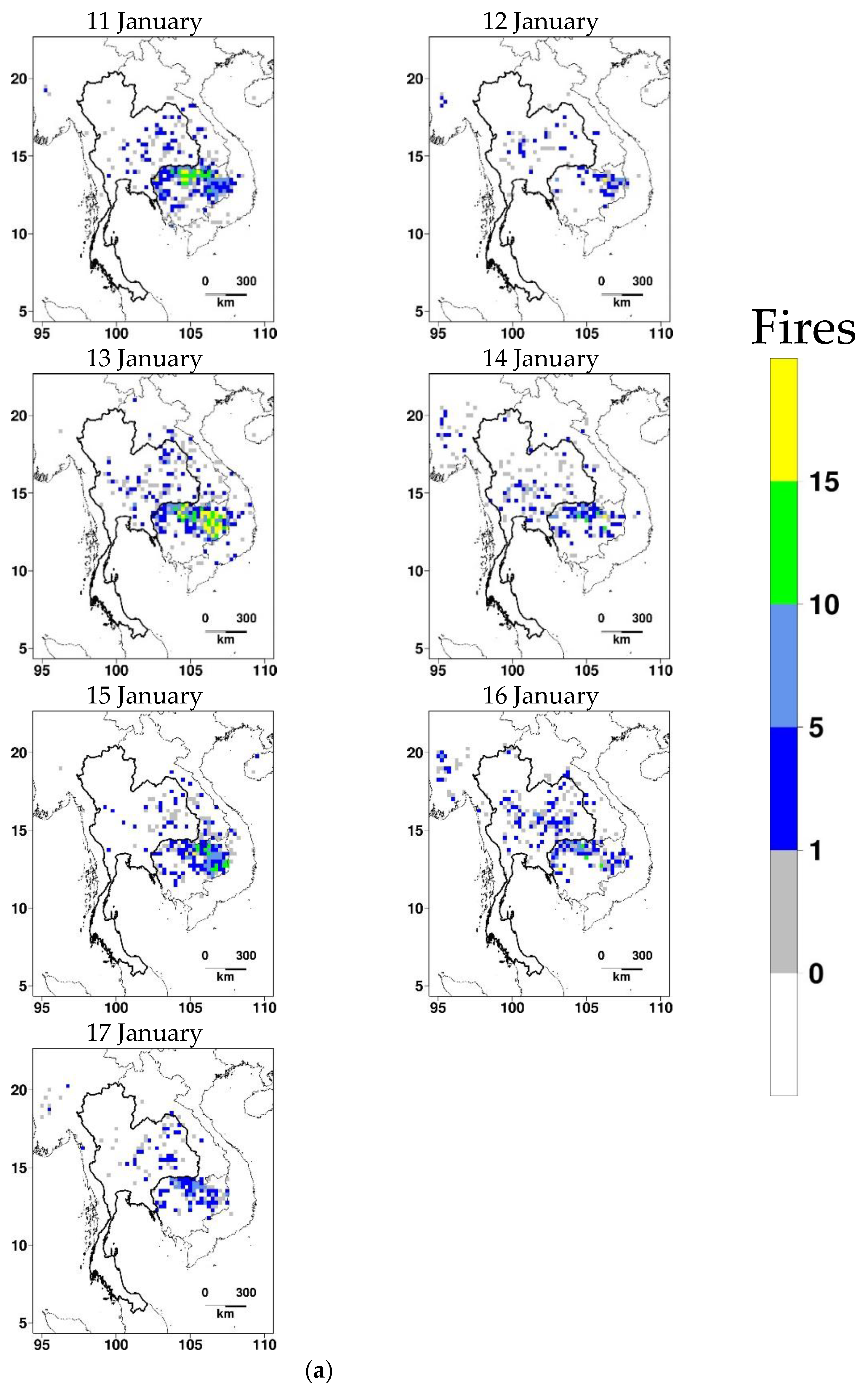
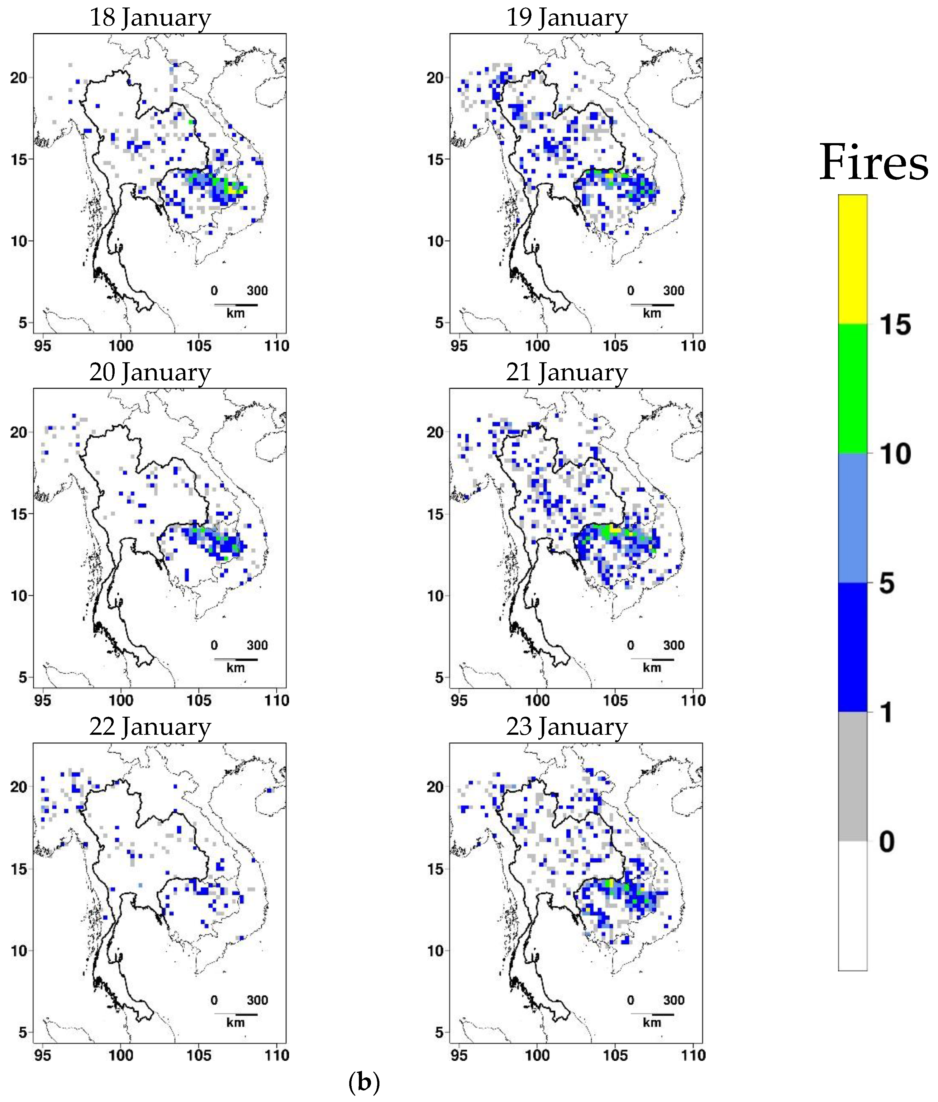
3.4. Effect of Biomass Burning
4. Discussion
5. Conclusions
Supplementary Materials
Author Contributions
Funding
Institutional Review Board Statement
Informed Consent Statement
Data Availability Statement
Acknowledgments
Conflicts of Interest
References
- Seinfeld, J.H.; Pandis, S.N. Atmospheric Chemistry and Physics from Air Pollution to Climate Change, 3rd ed.; John Wiley and Sons: New York, NY, USA, 2016; ISBN 978–1–118–94740–1. [Google Scholar]
- Zhang, R.; Wang, G.; Guo, S.; Zamora, M.L.; Ying, Q.; Lin, Y.; Wang, W.; Hu, M.; Wang, Y. Formation of urban fine particulate matter. Chem. Rev. 2015, 115, 3803–3855. [Google Scholar] [CrossRef] [PubMed]
- Health Effects Institute (HEI). State of Global Air 2020; A Special Report on Global Exposure to Air Pollution and Its Health Burden; Health Effects Institute, The Institute for Health Metrics and Evaluation, University of British Columbia, Boston, USA, 2018. Available online: https://www.stateofglobalair.org/sites/default/files/soga_2017_report.pdf (accessed on 8 January 2022).
- Lelieveld, J.; Evans, J.; Fnais, M.; Giannadaki, D.; Pozzer, A. The contribution of outdoor air pollution sources to premature mortality on a global scale. Nature 2015, 525, 367–371. [Google Scholar] [CrossRef] [PubMed]
- Huang, R.J.; Zhang, Y.; Bozzetti, C.; Ho, K.F.; Cao, J.J.; Han, Y.; Daellenbach, K.R.; Slowik, J.G.; Platt, S.M.; Canonaco, F.; et al. High secondary aerosol contribution to particulate pollution during haze events in China. Nature 2014, 514, 218–222. [Google Scholar] [CrossRef] [Green Version]
- Zhang, Y.L.; Cao, F. Fine particulate matter (PM2.5) in China at a city level. Sci. Rep. 2015, 5, 14884. [Google Scholar] [CrossRef] [PubMed] [Green Version]
- Aman, N.; Manomaiphiboon, K.; Pala-En, N.; Kokkaew, E.; Boonyoo, T.; Pattaramunikul, S.; Devkota, B.; Chotamonsak, C. Evolution of urban haze in Greater Bangkok and association with local meteorological and synoptic characteristics during two recent haze episodes. Int. J. Environ. Res. Public Health 2020, 17, 9499. [Google Scholar] [CrossRef]
- Aman, N.; Manomaiphiboon, K.; Pengchai, P.; Suwanathada, P.; Srichawana, J.; Assareh, N. Long–term observed visibility in eastern Thailand: Temporal variation, association with air pollutants and meteorological factors, and trends. Atmosphere 2019, 10, 122. [Google Scholar] [CrossRef] [Green Version]
- Mao, M.; Zhang, X.; Shao, Y.; Yin, Y. Spatiotemporal variations and factors of air quality in urban central China during 2013–2015. Int. J. Environ. Res. Public Health 2019, 17, 229. [Google Scholar] [CrossRef] [Green Version]
- Kumari, S.; Verma, N.; Lakhani, A.; Kumari, K.M. Severe haze events in the Indo–Gangetic Plain during post–monsoon: Synergetic effect of synoptic meteorology and crop residue burning emission. Sci. Total Environ. 2021, 768, 145479. [Google Scholar] [CrossRef]
- Chen, Z.; Chen, D.; Zhao, C.; Kwan, M.-P.; Cai, J.; Zhuang, Y.; Zhao, B.; Wang, X.; Chen, B.; Yang, J.; et al. Influences of meteorological conditions on PM2.5 concentrations across China: A review of methodology and mechanisms. Environ. Int. 2020, 139, 105558. [Google Scholar] [CrossRef]
- Pérez, I.A.; García, M.Á.; Sánchez, M.L.; Pardo, N.; Fernández-Duque, B. Key points in air pollution meteorology. Int. J. Environ. Res. Public Health 2020, 17, 8349. [Google Scholar] [CrossRef]
- Pollution Control Department (PCD). Thailand State of Pollution 2020; Pollution Control Department: Bangkok, Thailand, 2021; Available online: https://www.pcd.go.th/wp–content/uploads/2021/03/pcdnew–2021–04–07_06–54–58_342183.pdf (accessed on 19 September 2021).
- Chuersuwan, N.; Nimrat, S.; Lekphet, S.; Kerdkumrai, T. Levels and major sources of PM2.5 and PM10 in Bangkok Metropolitan Region. Environ. Int. 2008, 34, 671–677. [Google Scholar] [CrossRef] [PubMed]
- Wimolwattanapun, W.; Hopke, P.K.; Pongkiatkul, P. Source apportionment and potential source locations of PM2.5 and PM2.5–10 at residential sites in metropolitan Bangkok. Atmos. Pollut. Res. 2011, 2, 172–181. [Google Scholar] [CrossRef] [Green Version]
- ChooChuay, C.; Pongpiachan, S.; Tipmanee, D.; Suttinun, O.; Deelaman, W.; Wang, Q.; Li, X.; Li, G.; Han, Y.; Palakun, J.; et al. Impacts of PM2.5 sources on variations in particulate chemical compounds in ambient air of Bangkok, Thailand. Atmos. Pollut. Res. 2020, 11, 1657–1667. [Google Scholar] [CrossRef]
- Narita, D.; Oanh, N.T.K.; Sato, K.; Huo, M.; Permadi, D.A.; Chi, N.N.H.; Ratanajaratroj, T.; Pawarmart, I. Pollution characteristics and policy actions on fine particulate matter in a growing Asian economy: The case of Bangkok Metropolitan Region. Atmosphere 2019, 10, 227. [Google Scholar] [CrossRef] [Green Version]
- Phairuang, W.; Suwattiga, P.; Chetiyanukornkul, T.; Hongtieab, S.; Limpaseni, W.; Ikemori, F.; Hata, M.; Furuuchi, M. The influence of the open burning of agricultural biomass and forest fires in Thailand on the carbonaceous components in size–fractionated particles. Environ. Pollut. 2019, 247, 238–247. [Google Scholar] [CrossRef]
- Dejchanchaiwong, R.; Tekasakul, P.; Tekasakul, S.; Phairuang, W.; Nim, N.; Sresawasd, C.; Thongboon, K.; Thongyen, T.; Suwattiga, P. Impact of transport of fine and ultrafine particles from open biomass burning on air quality during 2019 Bangkok haze episode. J. Environ. Sci. 2020, 97, 238–247. [Google Scholar] [CrossRef]
- Aman, N.; Manomaiphiboon, K.; Suwattiga, P.; Assareh, N.; Limpaseni, W.; Suwanathada, P.; Soonsin, V.; Wang, Y. Visibility, aerosol optical depth, and low–visibility events in Bangkok during the dry season and associated local weather and synoptic patterns. Environ. Monit. Assess. 2022, 194, 322. [Google Scholar] [CrossRef]
- Stull, R.B. An Introduction to Boundary Layer Meteorology; Kluwer Academic Publishers: Dordrecht, Netherlands, 1998. [Google Scholar]
- Papanastasiou, D.K.; Melas, D. Climatology and impact on air quality of sea breeze in an urban coastal environment. Int. J. Climatol. 2009, 29, 305–315. [Google Scholar] [CrossRef]
- Chung-Shin, Y.; Bagtasa, G. Influence of local meteorology on the chemical characteristics of fine particulates in Metropolitan Manila in the Philippines. Atmos. Pollut. Res. 2020, 11, 1359–1369. [Google Scholar]
- Li, W.; Wang, Y.; Bernier, C.; Estes, M. Identification of sea breeze recirculation and its effects on ozone in Houston, TX, during DISCOVER–AQ 2013. J. Geophys. Res. Atmos. 2020, 125, e2020JD033165. [Google Scholar] [CrossRef]
- Miao, J.F.; Kroon, L.J.M.; Vilà-Guerau de Arellano, J.; Holtslag, A.A.M. Impacts of topography and land degradation on the sea breeze over eastern Spain. Meteorol. Atmos. Phys. 2003, 84, 157–170. [Google Scholar] [CrossRef]
- Abbs, D.J.; Physick, W.L. Sea breeze observations and modeling: A review. Aust. Meteorol. Mag. 1992, 41, 7–9. [Google Scholar]
- Wallance, J.M.; Hobbs, P.V. Atmospheric Science, 2nd ed.; Elsevier: New York, NY, USA, 2006; ISBN 978–0127329512. [Google Scholar]
- Arritt, R.W. Effects of the large–scale flow on characteristic features of the sea breeze. J. Appl. Meteor. 1993, 32, 116–125. [Google Scholar] [CrossRef]
- Azorin-Molina, C.; Chen, D. A climatological study of the influence of synoptic–scale flows on sea breeze evolution in the Bay of Alicante (Spain). Theor. Appl. Climatol. 2009, 96, 249–260. [Google Scholar] [CrossRef]
- Allende-Arandia, M.E.; Zavala-Hidalgo, J.; Torres-Freyermuth, A.; Appendini, C.M.; Cerezo-Mota, R.; Taylor-Espinosa, N. Sea–land breeze diurnal component and its interaction with a cold front on the coast of Sisal, Yucatan: A case study. Atmos. Res. 2020, 244, 105051. [Google Scholar] [CrossRef]
- Furberg, M.; Steyn, D.G.; Baldi, M. The climatology of sea breezes on Sardinia. Int. J. Climatol. 2002, 22, 917–932. [Google Scholar] [CrossRef]
- Hughes, C.P.; Veron, D.E. A characterization of the Delaware sea breeze using observations and modeling. J. Appl. Meteorol. Climatol. 2018, 57, 1405–1421. [Google Scholar] [CrossRef]
- Phan, T.T.; Manomaiphiboon, K. Observed and simulated sea breeze characteristics over Rayong coastal area, Thailand. Meteorol Atmos Phys. 2012, 116, 95–111. [Google Scholar] [CrossRef]
- Flocas, H.; Kelessis, A.; Helmis, C.; Petrakakis, M.; Zoumakis, M.; Pappas, K. Synoptic and local scale atmospheric circulation associated with air pollution episodes in an urban Mediterranean area. Theor. Appl. Climatol. 2009, 95, 265–277. [Google Scholar] [CrossRef]
- Mavrakou, T.; Philippopoulos, K.; Deligiorgi, D. The impact of sea breeze under different synoptic patterns on air pollution within Athens basin. Sci. Total Environ. 2012, 433, 31–43. [Google Scholar] [CrossRef]
- Ashfold, N.J.; Latif, M.T.; Samah, A.A.; Mead, M.I.; Harris, N.R.P. Influence of northeast monsoon cold surges on air quality in Southeast Asia. Atmos. Environ. 2017, 166, 498–509. [Google Scholar] [CrossRef] [Green Version]
- Hien, P.D.; Loc, P.D.; Dao, N.V. Air pollution episodes associated with East Asian winter monsoons. Sci. Total Environ. 2011, 409, 5063–5068. [Google Scholar] [CrossRef] [PubMed]
- Ly, B.T.; Matsumi, Y.; Nakayama, T.; Sakamoto, Y.; Kajii, Y.; Nghiem, T.D. Characterizing PM2.5 in Hanoi with new high temporal resolution sensor. Aerosol Air Qual. Res. 2018, 18, 2487–2497. [Google Scholar] [CrossRef]
- Wangwongchai, A.; Sixiong, Z.; Qingcun, Z. A case study on a strong tropical disturbance and record heavy rainfall in Hat Yai, Thailand during the winter monsoon. Adv. Atmos. Sci. 2005, 22, 436–450. [Google Scholar] [CrossRef]
- Wongsaming, P.; Exell, R.H.B. Criteria for forecasting cold surges associated with strong high pressure areas over Thailand during the winter monsoon. J. Sustain. Energy Environ. 2011, 2, 145–156. [Google Scholar]
- Department of Provincial Administration (DOPA). Statistic of Population by Province in 2020. 2021. Available online: https://stat.bora.dopa.go.th/new_stat/webPage/statByYear.php (accessed on 28 September 2021). (In Thai).
- National Economic and Social Development Board (NESDB). Gross Regional and Provincial Product, Chain Volume Measures: QGDP 1st Quarter 2020–4th Quarter 2020 Edition; Office of the National Economic and Social Development Board: Bangkok, Thailand, 2020; Available online: https://www.nesdc.go.th/nesdb_en/more_news.php?cid=155 (accessed on 28 September 2021).
- Land Development Department (LDD). Land Use and Land Cover Data for Thailand for the Years 2012–2016; CD–ROM Product; Land Development Department: Bangkok, Thailand, 2016. [Google Scholar]
- Thai Meteorological Department (TMD). The climate of Thailand. Thai Meteorological Department. 2021. Available online: https://www.tmd.go.th/en/archive/thailand_climate.pdf. (accessed on 28 September 2021).
- Zahumenský, I. Guidelines on Quality Control Procedures for Data from Automatic Weather Stations. World Meteorolgical Organziation. 2004. Available online: https://www.wmo.int/pages/prog/www/IMOP/meetings/Surface/ET–STMT1_Geneva2004/Doc6.1(2).pdf (accessed on 13 February 2021).
- Allwine, K.J.; Whiteman, C.D. Single–station integral measures of atmospheric stagnation, recirculation and ventilation. Atmos. Environ. 1994, 28, 713–721. [Google Scholar] [CrossRef]
- Bessho, K.; Date, K.; Hayashi, M.; Ikeda, A.; Imai, T.; Inoue, H.; Kumagai, Y.; Miyakawa, T.; Murata, H.; Ohno, T.; et al. An Introduction to Himawari–8/9—Japan’s New–Generation Geostationary Meteorological Satellites. J. Meteorol. Soc. Jpn. Ser. II 2016, 94, 151–183. [Google Scholar] [CrossRef] [Green Version]
- Chang, C.P.; Harr, P.A.; Chen, H.J. Synoptic disturbances over the equatorial South China Sea and western Maritime Continent during boreal winter. Mon. Weather Rev. 2005, 133, 489–503. [Google Scholar] [CrossRef]
- Hai, O.S.; Samah, A.A.; Chenoli, S.N.; Subramaniam, K.; Mazuki, M.Y.A. Extreme rainstorms that caused devastating flooding across the east coast of Peninsular Malaysia during November and December 2014. Weather Forecast. 2017, 32, 849–872. [Google Scholar] [CrossRef]
- Ryoo, S.B.; Kwon, W.T.; Jhun, J.G. Surface and upper–level features associated with wintertime cold surge outbreaks in South Korea. Adv. Atmos. Sci. 2005, 22, 509–524. [Google Scholar] [CrossRef]
- Wu, M.C.; Chan, J.C.L. Surface features of winter monsoon surges over South China. Mon. Weather Rev. 1995, 123, 662–680. [Google Scholar] [CrossRef]
- Chen, T.C.; Yen, M.C.; Huang, W.R.; Gallus, W.A. An East Asia cold surge: A case study. Mon. Weather Rev. 2002, 130, 2271–2290. [Google Scholar] [CrossRef]
- Borne, K.; Chen, D.; Nunez, M. A method for finding sea breeze days under stable synoptic conditions and its application to the Swedish west coast. Int. J. Climatol. 1998, 18, 901–914. [Google Scholar] [CrossRef]
- Giglio, L.; Schroeder, W.; Justice, C.O. The collection 6 MODIS active fire detection algorithm and fire products. Remote Sens. Environ. 2016, 178, 31–41. [Google Scholar] [CrossRef] [PubMed] [Green Version]
- Stein, A.F.; Draxler, R.R.; Rolph, G.D.; Stunder, B.J.B.; Cohen, M.D.; Ngan, F. NOAA’s HYSPLIT atmospheric transport and dispersion modeling system. Bull. Am. Meteorol. Soc. 2015, 96, 2059–2077. [Google Scholar] [CrossRef]
- Zhang, Q.; Quan, J.; Tie, X.; Li, X.; Liu, Q.; Gao, Y.; Zhao, D. Effects of meteorology and secondary particle formation on visibility during heavy haze events in Beijing, China. Sci. Total Environ. 2015, 502, 578–584. [Google Scholar] [CrossRef]
- Lovrić, M.; Antunović, M.; Šunić, I.; Vuković, M.; Kecorius, S.; Kröll, M.; Bešlić, I.; Godec, R.; Pehnec, G.; Geiger, B.C.; et al. Machine learning and meteorological normalization for assessment of particulate matter changes during the COVID-19 lockdown in Zagreb, Croatia. Int. J. Environ. Res. Public Health 2022, 19, 6937. [Google Scholar] [CrossRef]
- Onchang, R.; Hirunkasi, K.; Janchay, S. Establishment of a city-based index to communicate air pollution-related health risks to the public in Bangkok, Thailand. Sustainability 2022, 14, 16702. [Google Scholar] [CrossRef]
- Rattanapotanan, T.; Thongyen, T.; Bualert, S.; Choomanee, P.; Suwattiga, P.; Rungrattanaubon, T.; Utavong, T.; Phupijit, J.; Changplaiy, N. Secondary sources of PM2.5 based on the vertical distribution of organic carbon, elemental carbon, and water-soluble ions in Bangkok. Environ. Adv. 2023, 11, 100337. [Google Scholar] [CrossRef]
- Sun, J.; Gong, J.; Zhou, L.; Liu, J.; Liang, L. Analysis of PM2.5 pollution episodes in Beijing from 2014 to 2017: Classification, interannual variations and associations with meteorological features. Atmos. Environ. 2019, 213, 384–394. [Google Scholar] [CrossRef]
- Ma, Z.; Dey, S.; Christopher, S.; Liu, R.; Bi, J.; Balyan, P.; Liu, Y. A review of statistical methods used for developing large-scale and long-term PM2.5 models from satellite data. Remote Sens. Environ. 2022, 269, 112827. [Google Scholar] [CrossRef]


| Station | Coordinates (Latitude, Longitude) | Province | Variables | Background |
|---|---|---|---|---|
| P05 | 13.67, 100.61 | Bangkok | PM2.5, PM10, NOx, SO2, CO, T, RH, WS, WD | General area |
| P08 | 13.66, 100.54 | Samut Prakan | WS, WD | General area |
| P27 | 13.55, 100.26 | Samut Sakhon | PM2.5, PM10, T, GR | Mixed (roadside and general area) |
| P52 | 13.73, 100.49 | Bangkok | PM2.5, PM10, T, RH | Roadside |
| P61 | 13.77, 100.61 | Bangkok | PM2.5, PM10, T | General area |
| TMD (WMO484530) | 13.67, 100.61 | Bangkok | CC | General area |
| Duration (Days) | No. of Haze Episodes | No. of Episodes by Haze Type (I-II-III-IV) | Coefficient of Variation of Daily PM2.5 (Standard Deviation/Mean) |
|---|---|---|---|
| 1 | 11 | 0-4-0-7 | 0.1 |
| 2 | 7 | 0-5-2-0 | 0.16 |
| 3 | 3 | 0-2-0-1 | 0.1 |
| 4 | 3 | 0-1-2-0 | 0.12 |
| 5 | 2 | 0-2-0-0 | 0.21 |
| 6 | 2 | 1-0-1-0 | 0.1 |
| 7 | 2 | 1-1-0-0 | 0.09 |
| 8 | 2 | 2-0-0-0 | 0.15 |
| 10 | 2 | 0-0-2-0 | 0.16 |
| 11 | 1 | 0-0-1-0 | 0.29 |
| 13 | 2 | 0-0-2-0 | 0.21 |
| 14 | 1 | 0-0-1-0 | 0.25 |
| Total | 38 | 4-15-11-8 |
| Variable | Clean | Type I | Type II | Type III | Type IV |
|---|---|---|---|---|---|
| PM2.5 (μg m−3) | 31.3 ± 10.1 | 58.4 ± 1.8 | 56.8 ± 5.7 | 62.8 ± 6.4 | 54.1 ± 5.8 |
| T (°C) | 27.9 ± 1.5 | 26.9 ± 2.2 | 29.1 ± 0.7 | 27.6 ± 1.1 | 28.4 ± 1.3 |
| RH (%) | 64.1 ± 11.8 | 49.1 ± 4.8 | 59.1 ± 5.7 | 58.1 ± 6.3 | 58.2 ± 9.7 |
| CC (Fraction) | 6.0 ± 1.7 | 4.9 ± 1.5 | 5.1 ± 1.2 | 5.2 ± 1.5 | 5.5 ± 2.2 |
| GR (W m−2) | 428.6 ± 89.6 | 456.6 ± 36.9 | 471.1 ± 24.5 | 453.5 ± 40.5 | 414.1 ± 102.5 |
| RF (unitless) | 0.1 ± 0.2 | 0.1 ± 0.1 | 0.3 ± 0.2 | 0.3 ± 0.1 | 0.2 ± 0.1 |
| SB Duration (h) | 7.6 ± 4.0 | NA | 7.6 ± 3.2 | 6.2 ± 2.6 | 12.0 |
| SB Penetration (km) | 36.5 ± 35.8 | NA | 31.6 ± 25.3 | 20.5 ± 17.1 | 36.2 |
| Episode | Type | PM2.5/CO | NOx/CO | SO2/CO | |||
|---|---|---|---|---|---|---|---|
| Clean | Episodic | Clean | Episodic | Clean | Episodic | ||
| 1 | Type I | 56.5 | 57.2 | 55.9 | 53.1 | 2.9 | 2.5 |
| 6 | Type II | 56.5 | 63.6 | 55.9 | 54.5 | 2.9 | 2.7 |
| 7 | Type IV | 56.5 | 66.3 | 55.9 | 50.6 | 2.9 | 3.6 |
| 11 | Type IV | 56.5 | 83.8 | 55.9 | 52.2 | 2.9 | 2.9 |
| 12 | Type II | 66.4 | 79.1 | 59.9 | 54.5 | 2.7 | 4.2 |
| 16 | Type III | 66.4 | 83.4 | 59.9 | 50.61 | 2.7 | 2.5 |
| 21 | Type III | 52.8 | 57.1 | 50.3 | 48.6 | 1.7 | 1.8 |
| 22 | Type II | 52.8 | 63.7 | 50.3 | 44.8 | 1.7 | 1.7 |
| 25 | Type IV | 56.9 | 67.2 | 57.8 | 46.9 | 1.8 | 0.9 |
| 26 | Type II | 56.9 | 61.6 | 57.8 | 48.6 | 1.8 | 1.5 |
| 27 | Type I | 56.9 | 66.3 | 57.8 | 38.1 | 1.8 | 2.3 |
| 37 | Type II | 47.0 | 51.7 | 36.7 | 31.2 | 2.1 | – |
| 38 | Type II | 47.0 | 56.2 | 36.7 | 35.9 | 2.1 | – |
| Episode | Duration (Days) | No. of Days Affected by Biomass Burning (Day Number) | Impact |
|---|---|---|---|
| 04 | 1 | 1 (1st) | High |
| 07 | 1 | 1 (1st) | High |
| 08 | 5 | 1 (2nd) | Low |
| 10 | 10 | 4 (1st to 4th) | Low |
| 11 | 1 | 1 (1st) | High |
| 15 | 13 | 4 (4th, 6th, 8th and 13th) | Low |
| 16 | 14 | 5 (1st, 3rd, 4th, 10th and 14th) | Low |
| 18 | 10 | 1 (6th) | Low |
| 19 | 2 | 2 (1st and 2nd) | High |
| 20 | 4 | 1 (2nd) | Low |
| 21 | 13 | 4 (4th, 5th, 7th and 9th) | Low |
| 24 | 5 | (2nd and 5th) | Low |
| 25 | 3 | 2 (1st and 2nd) | High |
| 26 | 3 | 2 (2nd and 3rd) | High |
| 27 | 7 | 6 (1st, 2nd, 3rd, 4th, 5th and 6th) | High |
| 30 | 11 | 2 (4th and 9th) | Low |
| 32 | 1 | 1 (1st) | High |
| 33 | 2 | 1 (1st) | High |
| 37 | 2 | 2 (1st and 2nd) | High |
Disclaimer/Publisher’s Note: The statements, opinions and data contained in all publications are solely those of the individual author(s) and contributor(s) and not of MDPI and/or the editor(s). MDPI and/or the editor(s) disclaim responsibility for any injury to people or property resulting from any ideas, methods, instructions or products referred to in the content. |
© 2023 by the authors. Licensee MDPI, Basel, Switzerland. This article is an open access article distributed under the terms and conditions of the Creative Commons Attribution (CC BY) license (https://creativecommons.org/licenses/by/4.0/).
Share and Cite
Aman, N.; Manomaiphiboon, K.; Pala-En, N.; Devkota, B.; Inerb, M.; Kokkaew, E. A Study of Urban Haze and Its Association with Cold Surge and Sea Breeze for Greater Bangkok. Int. J. Environ. Res. Public Health 2023, 20, 3482. https://doi.org/10.3390/ijerph20043482
Aman N, Manomaiphiboon K, Pala-En N, Devkota B, Inerb M, Kokkaew E. A Study of Urban Haze and Its Association with Cold Surge and Sea Breeze for Greater Bangkok. International Journal of Environmental Research and Public Health. 2023; 20(4):3482. https://doi.org/10.3390/ijerph20043482
Chicago/Turabian StyleAman, Nishit, Kasemsan Manomaiphiboon, Natchanok Pala-En, Bikash Devkota, Muanfun Inerb, and Eakkachai Kokkaew. 2023. "A Study of Urban Haze and Its Association with Cold Surge and Sea Breeze for Greater Bangkok" International Journal of Environmental Research and Public Health 20, no. 4: 3482. https://doi.org/10.3390/ijerph20043482