
Mapping Health Fragility and Vulnerability in Air Pollution–Monitoring Networks in Dallas–Fort Worth


Abstract
:1. Introduction
2. Materials and Methods
3. Results
4. Discussion
5. Conclusions
Author Contributions
Funding
Institutional Review Board Statement
Informed Consent Statement
Data Availability Statement
Acknowledgments
Conflicts of Interest
References
- Landrigan, P.J.; Fuller, R.; Acosta, N.; Adeyi, O.; Arnold, R.; Basu, N.N.; Baldé, A.B.; Bertollini, R.; Bose-O’Reilly, S.; Boufford, J.I.; et al. The Lancet Commission on Pollution and Health. Lancet 2017, 391, 462–512. [Google Scholar] [CrossRef] [PubMed] [Green Version]
- Lefohn, A.S.; Jackson, W.; Shadwick, D.S.; Knudsen, H.P. Effect of surface ozone exposures on vegetation grown in the Southern Appalachian Mountains: Identification of possible areas of concern. Atmos. Environ. 1997, 31, 1695–1708. [Google Scholar] [CrossRef]
- U.S. Environmental Protection Agency (EPA). Air Sensors Guidebook. 2014. Available online: https://www.epa.gov/air-sensor-toolbox/how-use-air-sensors-air-sensor-guidebook (accessed on 25 March 2021).
- Lefohn, A.S.; Malley, C.S.; Smith, L.; Wells, B.; Hazucha, M.; Simon, H.; De Marco, A. Tropospheric ozone assessment report: Global ozone metrics for climate change, human health, and crop/ecosystem research. Elementa 2018, 1, 1. [Google Scholar] [CrossRef] [PubMed] [Green Version]
- Cutler, D.; Dominici, F. A breath of bad air: Cost of the Trump environmental agenda may lead to 80 000 extra deaths per decade. Jama 2018, 319, 2261–2262. [Google Scholar] [CrossRef] [Green Version]
- Northeim, K.; Marks, C.; Tiwari, C. Evaluating spatial patterns of seasonal ozone exposure and incidence of respiratory emergency room visits in Dallas—Fort Worth. PeerJ 2021, 10, e5678. [Google Scholar] [CrossRef]
- Jerrett, M.; Burnett, R.T.; Pope, C.A., III; Ito, K.; Thurston, G.; Krewski, D.; Shi, Y.; Calle, E.; Thun, M. Long-Term Ozone Exposure and Mortality. N. Engl. J. Med. 2009, 360, 1085–1095. [Google Scholar] [CrossRef] [Green Version]
- Caiazzo, F.; Ashok, A.; Waitz, I.A.; Yim, S.H.L.; Barrett, S.R.H. Air Pollution and Early Deaths in the United States. Part I: Quantifying the Impact of Major Sectors in 2005. Atmos. Environ. 2013, 79, 198–208. [Google Scholar]
- Duyzer, J.; van den Hout, D.; Zandveld, P.; van Ratingen, S. Representativeness of air quality monitoring networks. Atmos. Environ. 2015, 104, 88–101. [Google Scholar] [CrossRef]
- Shahraiyni, H.T.; Sodoudi, S.; Kerschbaumer, A.; Cubasch, U. New technique for ranking of air pollution monitoring stations in the urban areas based upon spatial representativity (Case study: PM monitoring stations in Berlin). Aerosol Air Qual. Res. 2015, 15, 743–748. [Google Scholar] [CrossRef] [Green Version]
- Reames, T.G.; Bravo, M.A. People, place and pollution: Investigating relationships between air quality perceptions, health concerns, exposure, and individual-and area-level characteristics. Environ. Int. 2019, 122, 244–255. [Google Scholar] [CrossRef] [PubMed]
- U.S. Environmental Protection Agency (EPA). Electronic Federal Records. 2021. Available online: https://www.ecfr.gov/cgi-bin/retrieveECFR?gp=&r=PART&n=40y6.0.1.1.6 (accessed on 27 March 2021).
- Koman, P.D.; Hogan, K.A.; Sampson, N.; Mandell, R.; Coombe, C.M.; Tetteh, M.M.; Woodruff, T.J. Examining Joint Effects of Air Pollution Exposure and Social Determinants of Health in Defining “At-Risk” Populations Under the Clean Air Act: Susceptibility of Pregnant Women to Hypertensive Disorders of Pregnancy. World Med. Health Policy 2018, 10, 7–54. [Google Scholar] [CrossRef]
- Miranda, M.L.; Edwards, S.E.; Keating, M.H.; Paul, C.J. Making the environmental justice grade: The relative burden of air pollution exposure in the United States. Int. J. Environ. Res. Public Health 2011, 8, 1755–1771. [Google Scholar] [CrossRef] [PubMed]
- Medina-Ramon, M.; Schwartz, J. Who is more vulnerable to die from ozone air pollution? Epidemiology 2008, 19, 672–679. [Google Scholar] [CrossRef] [PubMed]
- Oppong, J.R. A vulnerability interpretation of the geography of HIV/AIDS in Ghana, 1986–1995. Prof. Geogr. 1998, 50, 437–448. [Google Scholar] [CrossRef]
- Makri, A.; Stilianakis, N.I. Vulnerability to air pollution health effects. Int. J. Hyg. Environ. Health 2008, 211, 326–336. [Google Scholar] [CrossRef]
- World Health Organization (WHO). 2018. Available online: https://www.who.int/news-room/detail/02-05-2018-9-out-of-10-people-worldwide-breathe-polluted-air-but-more-countries-are-taking-action (accessed on 17 October 2019).
- Flanagan, B.; Hallisey, E.; Adams, E.; Lavery, A. Measuring Community Vulnerability to Natural and Anthropogenic Hazards: The Centers for Disease Control and Prevention’s Social Vulnerability Index. J. Environ. Health 2018, 80, 34–36. [Google Scholar]
- Cutter, S. Vulnerability to environmental hazards. Hum. Geogr. 1996, 20, 529–539. [Google Scholar] [CrossRef]
- Cutter, S.; Mitchell, J.; Scott, M. Revealing the Vulnerability of People and Places: A Case Study of Georgetown County, South Carolina. Ann. Assoc. Am. Geogr. 2000, 90, 713–737. [Google Scholar] [CrossRef]
- Cutter, S.; Emrich, C.; Mitchell, J.; Boruff, B.; Gall, M.; Schmidtlein, M.; Burton, C.; Melton, G. The Long Road Home: Race, Class, and Recovery from Hurricane Katrina. Environ. Sci. Policy Sustain. Dev. 2006, 48, 10–20. [Google Scholar] [CrossRef]
- Oppong, J.R.; Harold, A. Disease, Ecology and Environment. In A Companion to Health and Medical Geography; Brown, T., McLafferty, S., Moon, G., Eds.; Blackwell-Wiley: Chichester, UK, 2010. [Google Scholar]
- Sabrin, S.; Karimi, M.; Nazari, R. Developing Vulnerability Index to Quantify Urban Heat Islands Effects Coupled with Air Pollution: A Case Study of Camden, NJ. ISPRS Int. J. Geo-Inf. 2020, 9, 349. [Google Scholar] [CrossRef]
- Wright, C.Y.; Diab, R. Air Pollution and Vulnerability: Solving the Puzzle of Prioritization. J. Environ. Health 2011, 73, 55–56. [Google Scholar]
- Mahady, J.A.; Octaviano, C.; Araiza Bolaños, O.S.; López, E.R.; Kammen, D.M.; Castellanos, S. Mapping Opportunities for Transportation Electrification to Address Social Marginalization and Air Pollution Challenges in Greater Mexico City. Environ. Sci. Technol. 2020, 54, 2103–2111. [Google Scholar] [CrossRef] [PubMed] [Green Version]
- U.S. Center for Disease Control (CDC). CDC SVI Fact Sheet. 2021. Available online: https://www.atsdr.cdc.gov/placeandhealth/svi/fact_sheet/fact_sheet.html (accessed on 3 March 2021).
- Texas Center for Environmental Quality (TCEQ). Dallas-Fort Worth: Current Attainment Status. 2022. Available online: https://www.tceq.texas.gov/airquality/sip/dfw/dfw-status (accessed on 28 December 2022).
- U.S. Environmental Protection Agency (EPA). Ozone National Ambient Air Quality Standards. 2022. Available online: https://www.epa.gov/ground-level-ozone-pollution/ozone-national-ambient-air-quality-standards-naaqs (accessed on 29 December 2022).
- American Community Survey (ACS). 2018 Data Release; New and Notable. Available online: https://www.census.gov/programs-surveys/acs/news/data-releases/2018/release.html (accessed on 25 March 2021).
- Northeim, K.; Tiwari, C.; Oppong, J. Surface ozone monitoring and policy: A geospatial decision support tool for suitable location of monitoring stations in urban areas. Environ. Sci. Policy 2021, 126, 48–59. [Google Scholar] [CrossRef]
- Diem, J.E. A critical examination of ozone mapping from a spatial-scale perspective. Environ. Pollut. 2003, 125, 369–383. [Google Scholar] [CrossRef]
- Pope, C.A., 3rd. Epidemiology of fine particulate air pollution and human health: Biologic mechanisms and who’s at risk? Environ. Health Perspect. 2000, 108 (Suppl. S4), 713–723. [Google Scholar] [CrossRef] [PubMed]
- Charafeddine, R.; Boden, L.I. Does income inequality modify the association between air pollution and health? Environ. Res. 2008, 106, 81–88. [Google Scholar] [CrossRef] [PubMed]
- U.S. Center for Disease Control (CDC). CDC SVI Fact Sheet. 2022. Available online: https://www.atsdr.cdc.gov/placeandhealth/svi/documentation/pdf/SVI2018Documentation-H.pdf (accessed on 18 December 2022).
- Kanaroglou, P.S.; Jerrett, M.; Morrison, J.; Beckerman, B.; Arain, M.A.; Gilbert, N.L.; Brook, J.R. Establishing an air pollution monitoring network for intra-urban population exposure assessment: A location-allocation approach. Atmos. Environ. 2005, 39, 2399–2409. [Google Scholar] [CrossRef]
- Frumkin, H. Urban Sprawl and Public Health. Public Health Rep. 2002, 117, 201–217. [Google Scholar] [CrossRef]
- Seilkop, S.K.; Campen, M.J.; Lund, A.K.; McDonald, J.D.; Mauderly, J.L. Identification of Chemical Components of Combustion Emissions that Affect Pro-Atherosclerotic Vascular Responses in Mice. Inhal. Toxicol. 2012, 24, 270–287. [Google Scholar] [CrossRef]
- Simoni, M.; Baldacci, S.; Maio, S.; Cerrai, S.; Sarno, G.; Viegi, G. Adverse effects of outdoor pollution in the elderly. J. Thorac. Dis. 2015, 7, 34. [Google Scholar]
- Conway, M.; Shakya, K.; Kremer, P. Mapping Social Vulnerability to Air Pollution in Philadelphia, PA. Veritas Villanova Res. J. 2020, 2, 122–130. [Google Scholar]
- Karaye, I.M.; Horney, J.A. The impact of social vulnerability on COVID-19 in the US: An analysis of spatially varying relationships. Am. J. Prev. Med. 2020, 59, 317–325. [Google Scholar] [CrossRef] [PubMed]
- Ge, Y.; Zhang, H.; Dou, W.; Chen, W.; Liu, N.; Wang, Y.; Rao, W. Mapping social vulnerability to air pollution: A case study of the Yangtze River Delta region, China. Sustainability 2017, 9, 109. [Google Scholar] [CrossRef] [Green Version]
- U.S. Census. The Urban and Rural Classifications. 2021. Available online: https://www2.census.gov/geo/pdfs/reference/GARM/Ch12GARM.pdf (accessed on 3 July 2021).
- Matthews, K.A.; Croft, J.B.; Liu, Y.; Lu, H.; Kanny, D.; Wheaton, A.G.; Cunningham, T.J.; Khan, L.K.; Caraballo, R.S.; Holt, J.B.; et al. Health-related behaviors by urban-rural county classification—United States, 2013. MMWR Surveill. Summ. 2017, 66, 1. [Google Scholar] [CrossRef] [PubMed]
- Marsden, T. Beyond the Rural-Urban Divide: Cross-Continental Perspectives on the Differentiated Countryside and Its Regulation; Emerald Group Publishing: Bingley, UK, 2009. [Google Scholar]
- Douthit, N.; Kiv, S.; Dwolatzky, T.; Biswas, S. Exposing some important barriers to health care access in the rural USA. Public Health 2015, 129, 611–620. [Google Scholar] [CrossRef] [PubMed]
- Ahmadi, M.; John, K. Statistical evaluation of the impact of shale gas activities on ozone pollution in North Texas. Sci. Total Environ. 2015, 536, 457–467. [Google Scholar] [CrossRef] [PubMed]
- Texas Center for Environmental Quality (TCEQ). Air Quality Monitoring. 2023. Available online: https://www.tceq.texas.gov/airquality/monops/ (accessed on 12 January 2023).


| Scale | Not Covered = Outside Spatial Scale | Covered = Inside Spatial Scale | ||
|---|---|---|---|---|
| Variable | Description | Variable | Description | |
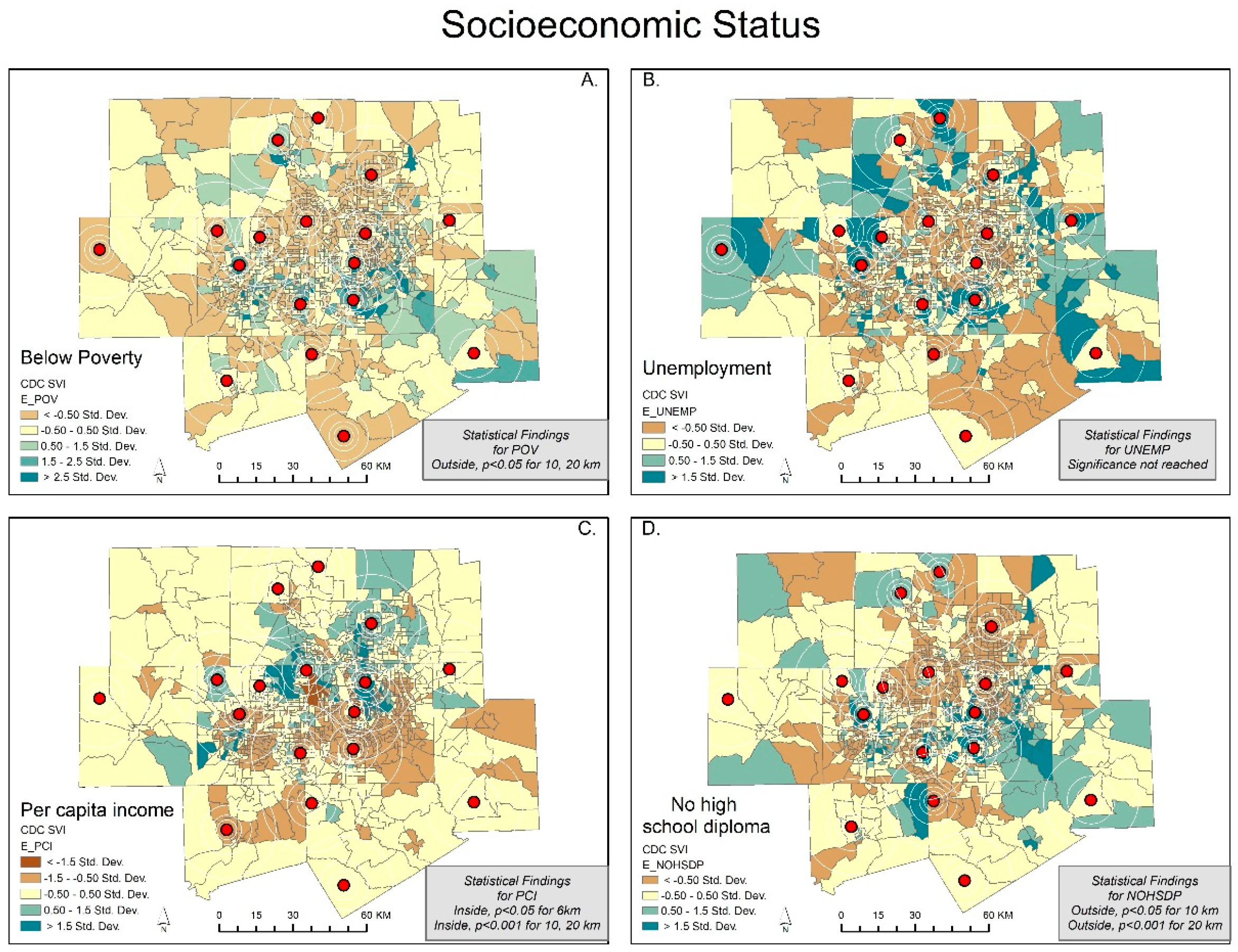
| 4 km | – | not significant | – | not significant |
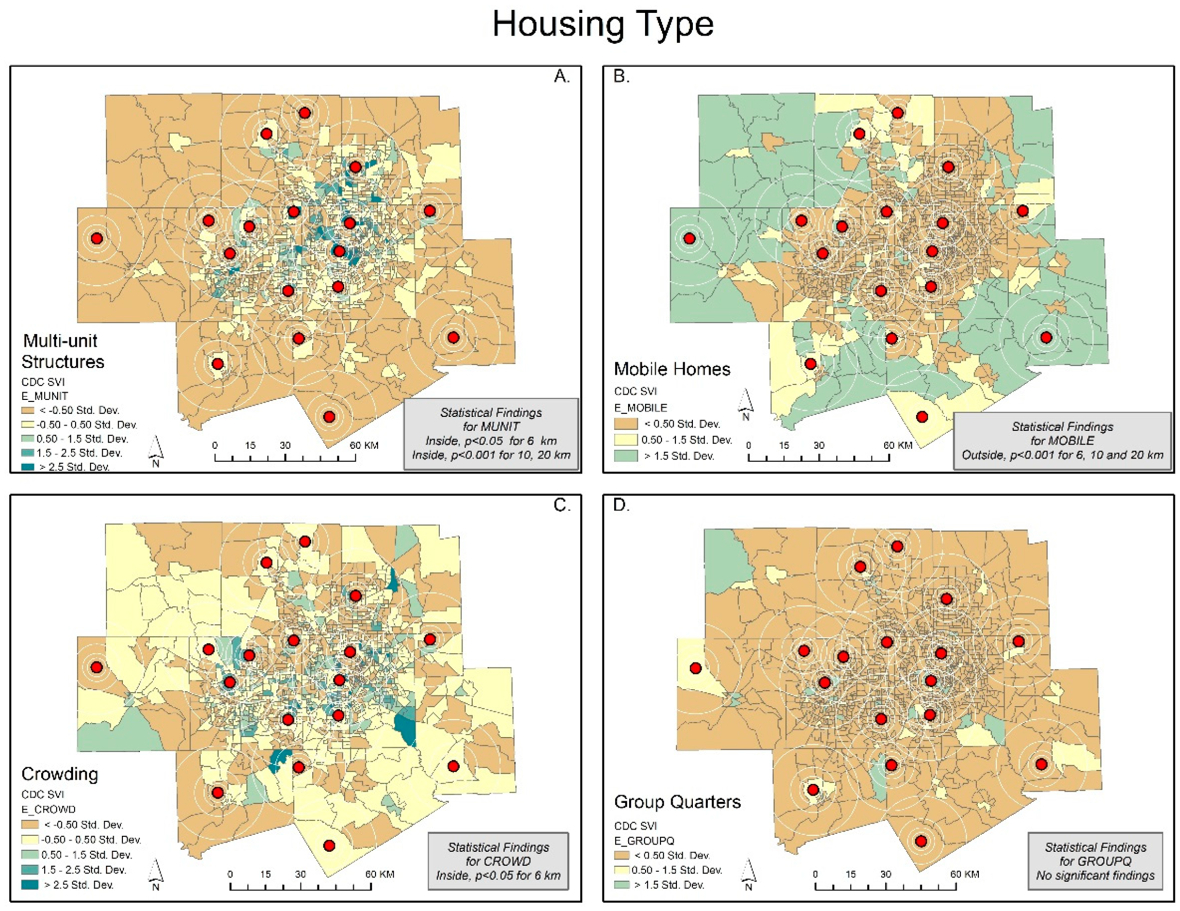
| 6 km | E_MOBILE ** | Mobile homes | E_PCI * | Per capita income |
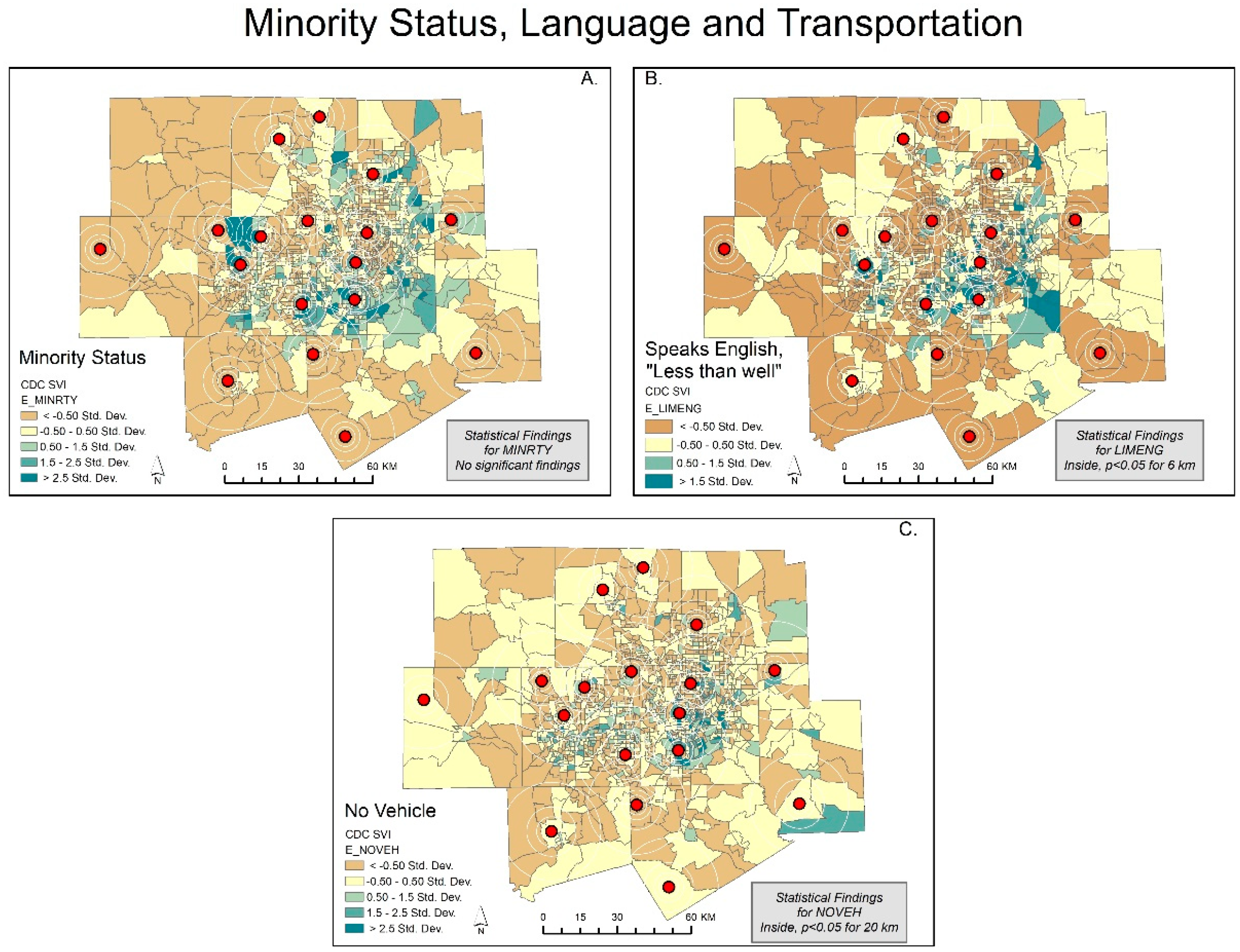
| E_LIMENG * | Speaks English “less than well” | |||
| E_MUNIT * | Multiunit structures | |||
| E_CROWD * | Crowding | |||
| 10 km | E_POV * | Below Poverty | E_PCI ** | Per capita income |
| E_NOHSDP * | No High School Diploma | E_MUNIT ** | Multiunit structures | |
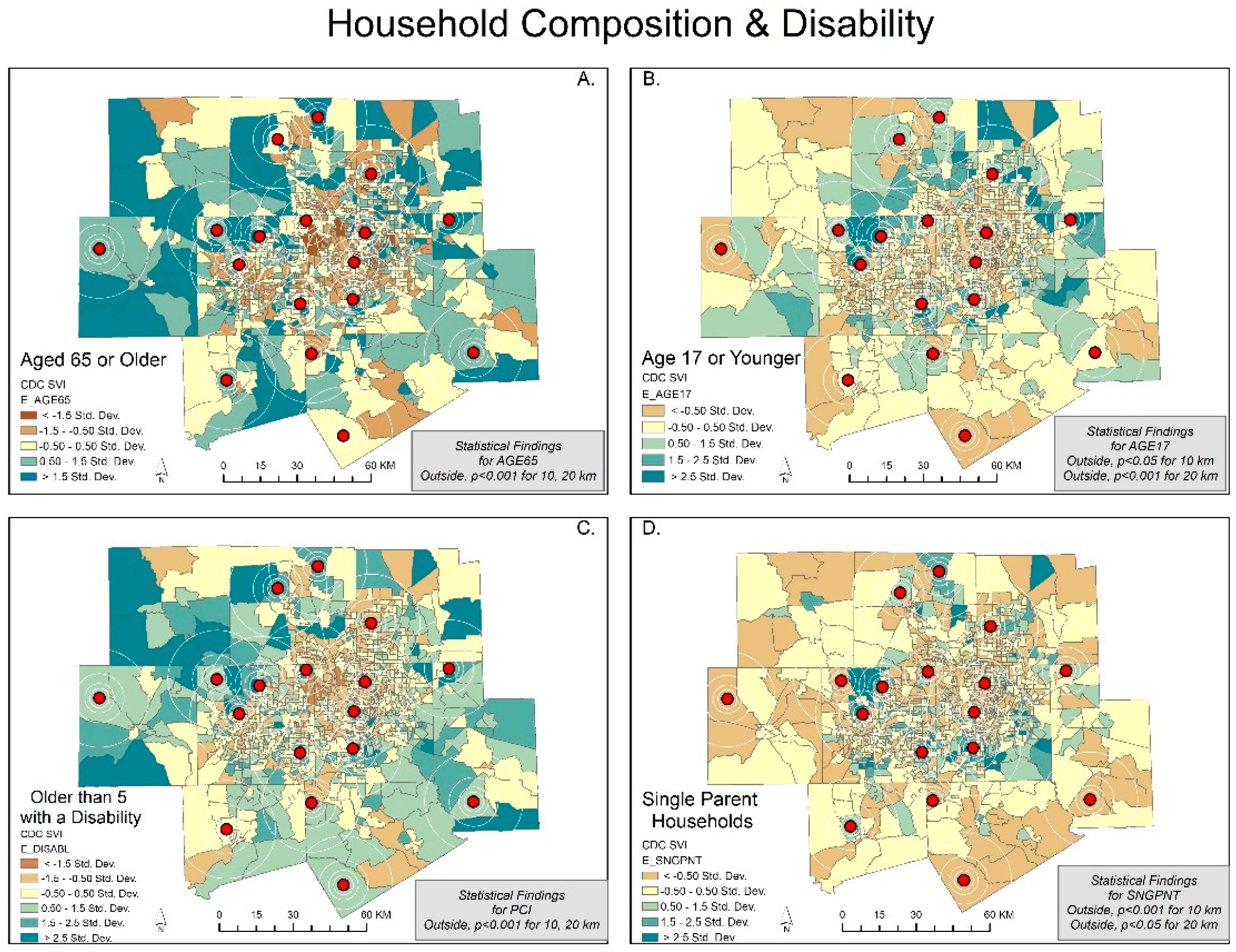
| E_AGE65 ** | Aged 65 or Older | |||
| E_AGE17 * | Aged 17 or Younger | |||
| E_DISABL ** | Older than Age 5 with a Disability | |||
| E_SNGPNT * | Single-Parent Households | |||
| E_MOBILE ** | Mobile Homes | |||
| 20 km | E_POV * | Below Poverty | E_PCI ** | Per capita income |
| E_NOHSDP ** | No High School Diploma | E_MUNIT ** | Multiunit structures | |
| E_AGE65 ** | Aged 65 or Older | E_NOVEH * | No Vehicle | |
| E_AGE17 ** | Aged 17 or Younger | |||
| E_DISABL ** | Older than Age 5 with a Disability | |||
| E_SNGPNT * | Single-Parent Households | |||
| E_MOBILE ** | Mobile Homes | |||
| Variable | Description | Odds Ratio (95% CI) | |
|---|---|---|---|
| – | 10 km | 20 km | |
| F_POV | Below Poverty | 0.563 (0.288–1.101) | 0.619 (0.142–2.694) |
| F_UNEMP | Unemployment | 0.847 (0.485–1.481) | 0.585 (0.169–2.024) |
| F_PCI | Per Capita Income | 1.753 (0.913–3.3640) | 1.138 (0.377–3.437) |
| F_NOHSDP | No High School Diploma | 0.958 (0.541–1.697) | 1.715 (0.638–4.613) |
| F_AGE65 | Aged 65 or Older | 0.955 (0.576–1.583) | 0.841 (0.304–2.326) |
| F_AGE17 | Aged 17 or Younger | 1.018 (0.679–1.528) | 2.177 (1.159–4.092) |
| F_DISABL | Older than Age 5 with a Disability | 0.717 (0.302–1.700) | 2.189 (0.498–9.628) |
| F_SNGPNT | Single-Parent Households | 1.886 (1.242–2.863) | 2.094 (1.066–4.117) |
| F_MINRTY | Minority Status | 0.939 (0.524–1.682) | 0.493 (0.142–1.711) |
| F_LIMENG | Speaks English “Less Than Well” | 0.521 (0.292–0.931) | 0.762 (0.259–2.242) |
| F_MUNIT | Multiunit Structures | 0.392 (0.281–0.548) | 0.130 (0.037–0.457) |
| F_MOBILE | Mobile Homes | 4.831 (2.500–9.338) | 8.066 (4.390–14.820) |
| F_CROWD | Crowding | 0.972 (0.609–1.549) | 0.453 (0.174–1.176) |
| F_NOVEH | No Vehicle | 1.467 (0.885–2.432) | 0.367 (0.091–1.479) |
| F_GROUPQ | Group Quarters | 0.723 (0.432–1.209) | 2.593 (1.224–5.493) |
Disclaimer/Publisher’s Note: The statements, opinions and data contained in all publications are solely those of the individual author(s) and contributor(s) and not of MDPI and/or the editor(s). MDPI and/or the editor(s) disclaim responsibility for any injury to people or property resulting from any ideas, methods, instructions or products referred to in the content. |
© 2023 by the authors. Licensee MDPI, Basel, Switzerland. This article is an open access article distributed under the terms and conditions of the Creative Commons Attribution (CC BY) license (https://creativecommons.org/licenses/by/4.0/).
Share and Cite
Northeim, K.; Oppong, J.R. Mapping Health Fragility and Vulnerability in Air Pollution–Monitoring Networks in Dallas–Fort Worth. Int. J. Environ. Res. Public Health 2023, 20, 1807. https://doi.org/10.3390/ijerph20031807
Northeim K, Oppong JR. Mapping Health Fragility and Vulnerability in Air Pollution–Monitoring Networks in Dallas–Fort Worth. International Journal of Environmental Research and Public Health. 2023; 20(3):1807. https://doi.org/10.3390/ijerph20031807
Chicago/Turabian StyleNortheim, Kari, and Joseph R. Oppong. 2023. "Mapping Health Fragility and Vulnerability in Air Pollution–Monitoring Networks in Dallas–Fort Worth" International Journal of Environmental Research and Public Health 20, no. 3: 1807. https://doi.org/10.3390/ijerph20031807