
Social Factors as Major Determinants of Rural Development Variation for Predicting Epidemic Vulnerability: A Lesson for the Future


Abstract
:1. Introduction
2. Materials and Methods
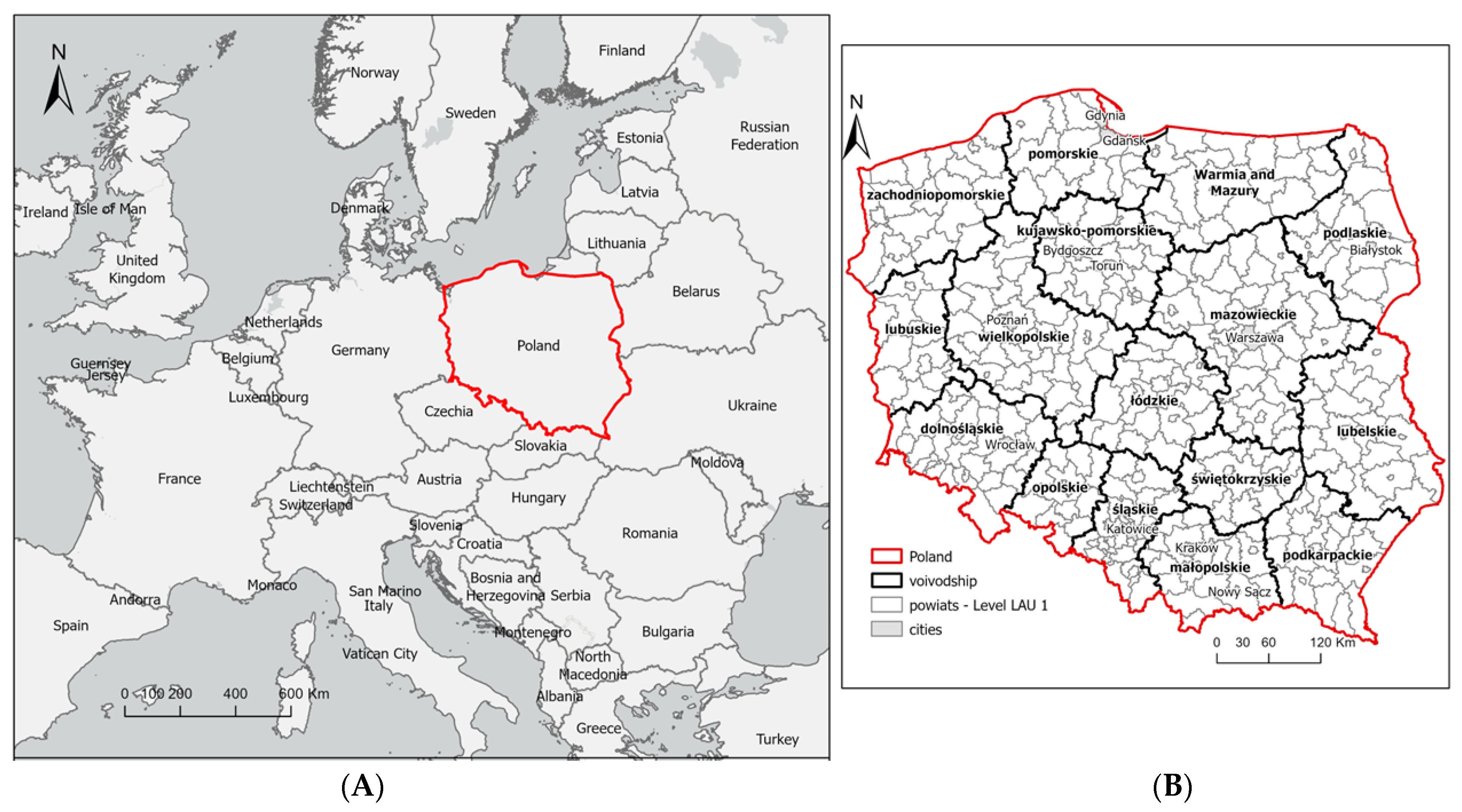
2.1. Materials
2.2. Methods

| Factor | Social Interactions | Type of Factor | Factor Selection | Literature Subject | |||||
|---|---|---|---|---|---|---|---|---|---|
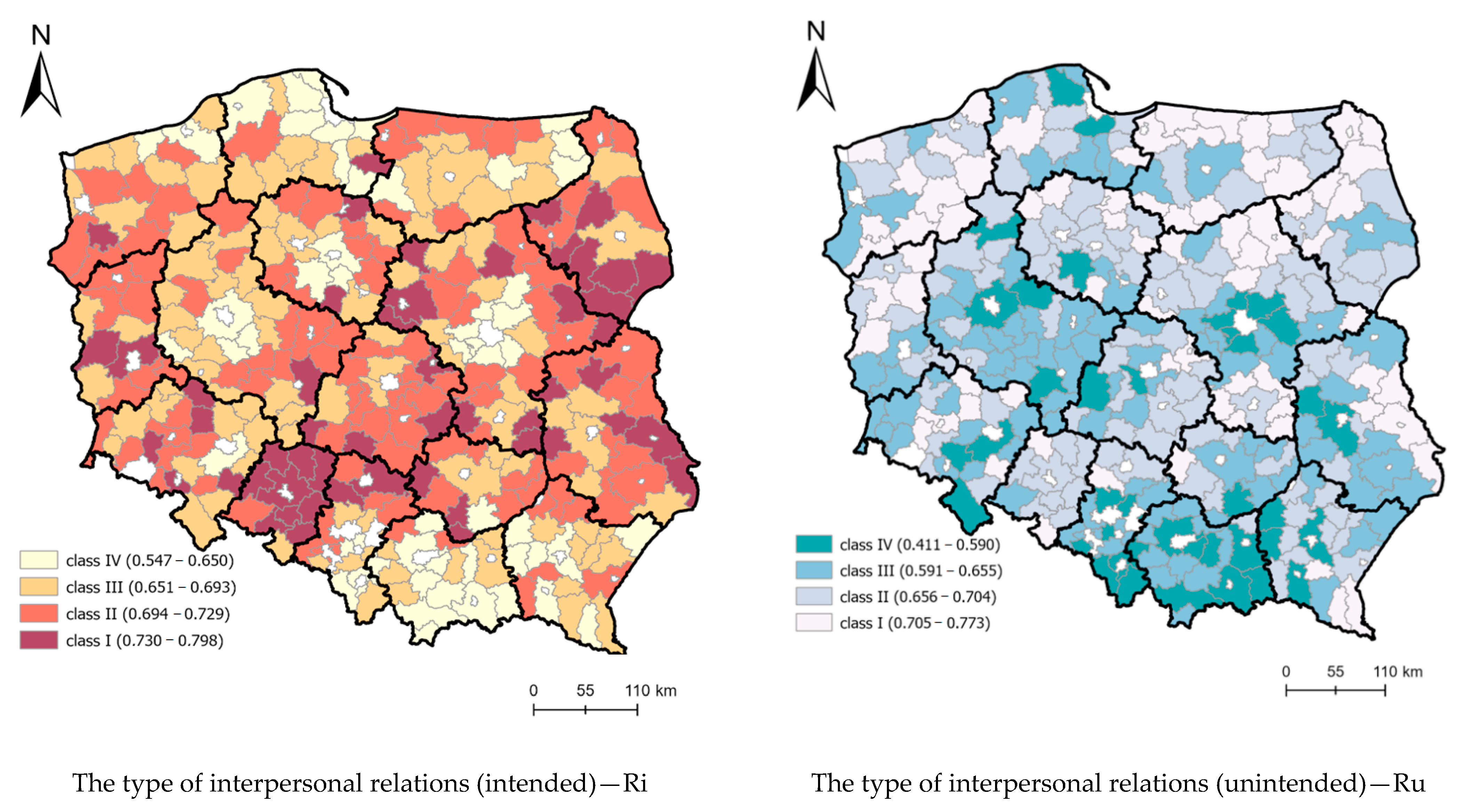
| Nature of the Factors | Type of Interpersonal and Social Relations | ||||||||
| D | S | L | E | I | U | ||||
| X1—population per 1 km2 | x | x | x | destimulant | accept | [32,52] | |||
| X2—share of population aged 6–19 years and more (%) | x | x | destimulant | accept | [53] | ||||
| X3—share of population aged 60 and over (%) | x | x | x | destimulant | reject | [32] | |||
| X4—population per township | x | x | destimulant | reject | [32,52] | ||||
| X5—balance of internal migration per 1000 population | x | x | x | destimulant | accept | [17,32] | |||
| X6—balance of foreign migration per 1000 population | x | x | x | destimulant | accept | [17] | |||
| X7—registered unemployment rate (%) | x | x | stimulant | accept | [17,32,52] | ||||
| X8—average number of persons per 1 apartment | x | x | destimulant | reject | [32,52] | ||||
| X9—average number of persons per 1 room | x | x | destimulant | accept | [32,52] | ||||
| X10—number of accommodation establishments over 10 people | x | x | x | destimulant | reject | [17,32] | |||
| X11—number of vehicles per 1000 population | x | x | destimulant | accept | [32,52] | ||||
| X12—hypermarkets (number) | x | x | destimulant | accept | [54] | ||||
| X13—supermarkets (number) | x | x | destimulant | reject | [54] | ||||
| X14—marketplaces (number) | x | x | destimulant | accept | [54] | ||||
| X15—village centers (number) | x | x | destimulant | reject | [54] | ||||
| X16—events (number) | x | x | destimulant | reject | [55] | ||||
| X17—number of event attendees per 1000 population | x | x | destimulant | accept | [55] | ||||
| X18—number of people per facility (cultural center, community center, club, community hall) | x | x | destimulant | accept | [55] | ||||
| X19—number of beds in sanatoria | x | x | destimulant | reject | [54] | ||||
| X20—population density in housing areas (person/1 km2) * | x | x | destimulant | accept | [56] | ||||
| X21—population density of built-up and urbanized areas (person/km2) * | x | x | destimulant | accept | [56,57] | ||||
| X22—average useful floor area of a dwelling per 1 person | x | x | stymulant | reject | [57,58] | ||||
| X23—population density of industrial areas (person/1 km2) * | x | x | x | destimulant | accept | [17,57,58] | |||
| X24—number of towns | x | x | destimulant | accept | [58] | ||||
| X25—business entities by size classes per 1000 inhabitants in total | x | x | x | destimulant | accept | [17] | |||
| X26—ambulatory health care—medical consultations per 1000 population | x | x | destimulant | Reject | [59] | ||||
| X27—physicians (total working staff) per 10,000 population | x | x | destimulant | accept | [59] | ||||
| X28—residents of nursing homes per 1000 inhabitants | x | x | destimulant | accept | [60] | ||||
| X29—children in pre-school education establishments per 1000 children aged 3–5 years | x | x | destimulant | accept | [61] | ||||
| X30—national economy entities employing more than 49 persons per 10 thousand population | x | x | x | destimulant | reject | [17] | |||
| X31—number of bed places per 1000 population | x | x | x | destimulant | reject | [17,32] | |||
| X32—tourists using accommodation per 1000 population | x | x | destimulant | accept | [17,32] | ||||
| X33—% degree of utilisation of accommodation% | x | x | x | destimulant | accept | [17,32] | |||
3. Results of Empirical Surveys
4. Discussion
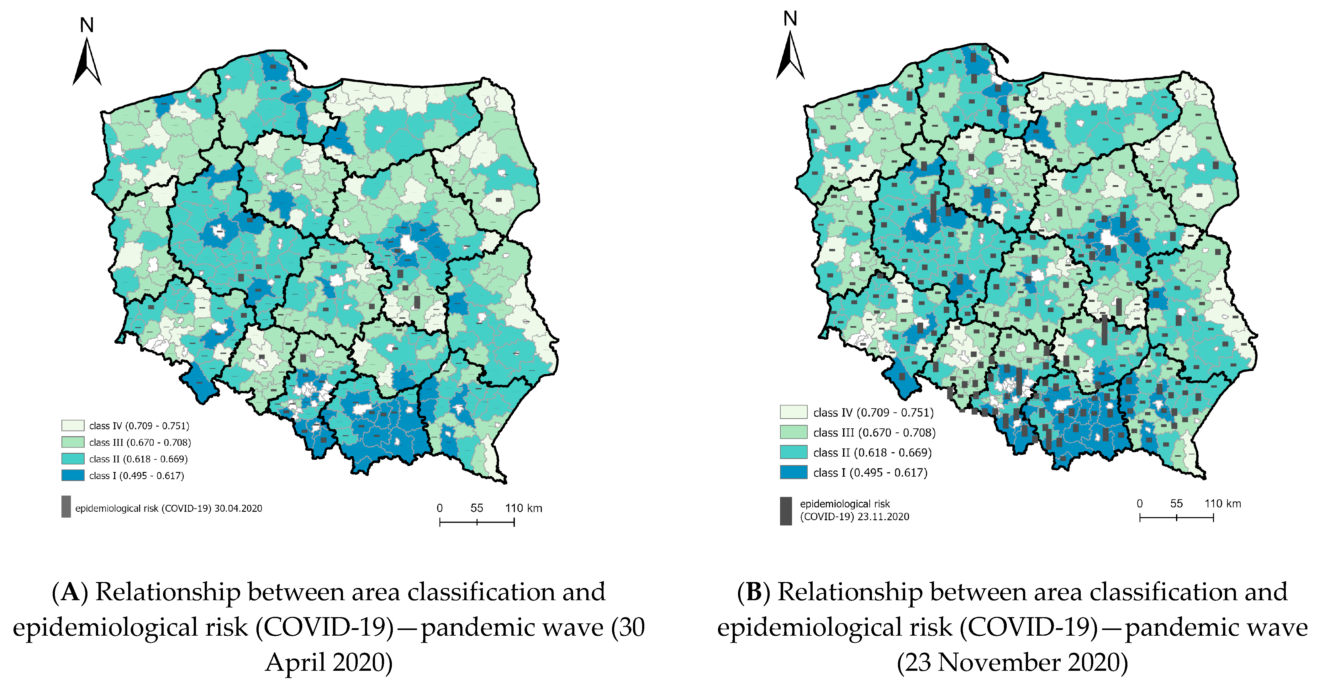
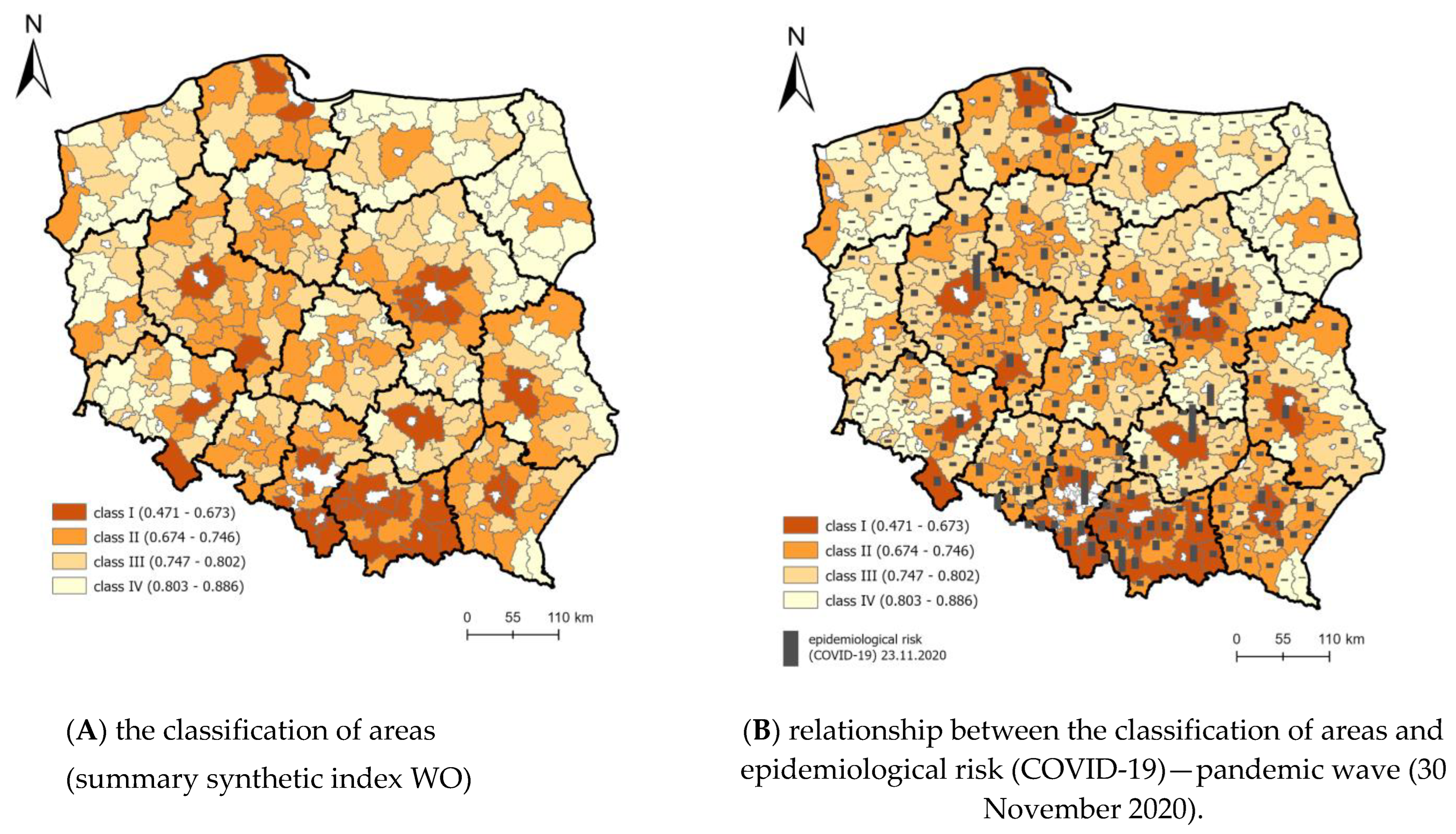
4.1. Strength of the Relationship between the Classification of Areas in the KLE Model and the Spread of COVID-19
4.2. Correlation between Component Models and the COVID-19 Spread Pattern
4.3. Revised Model of Vulnerability to Epidemic Threats—Poland
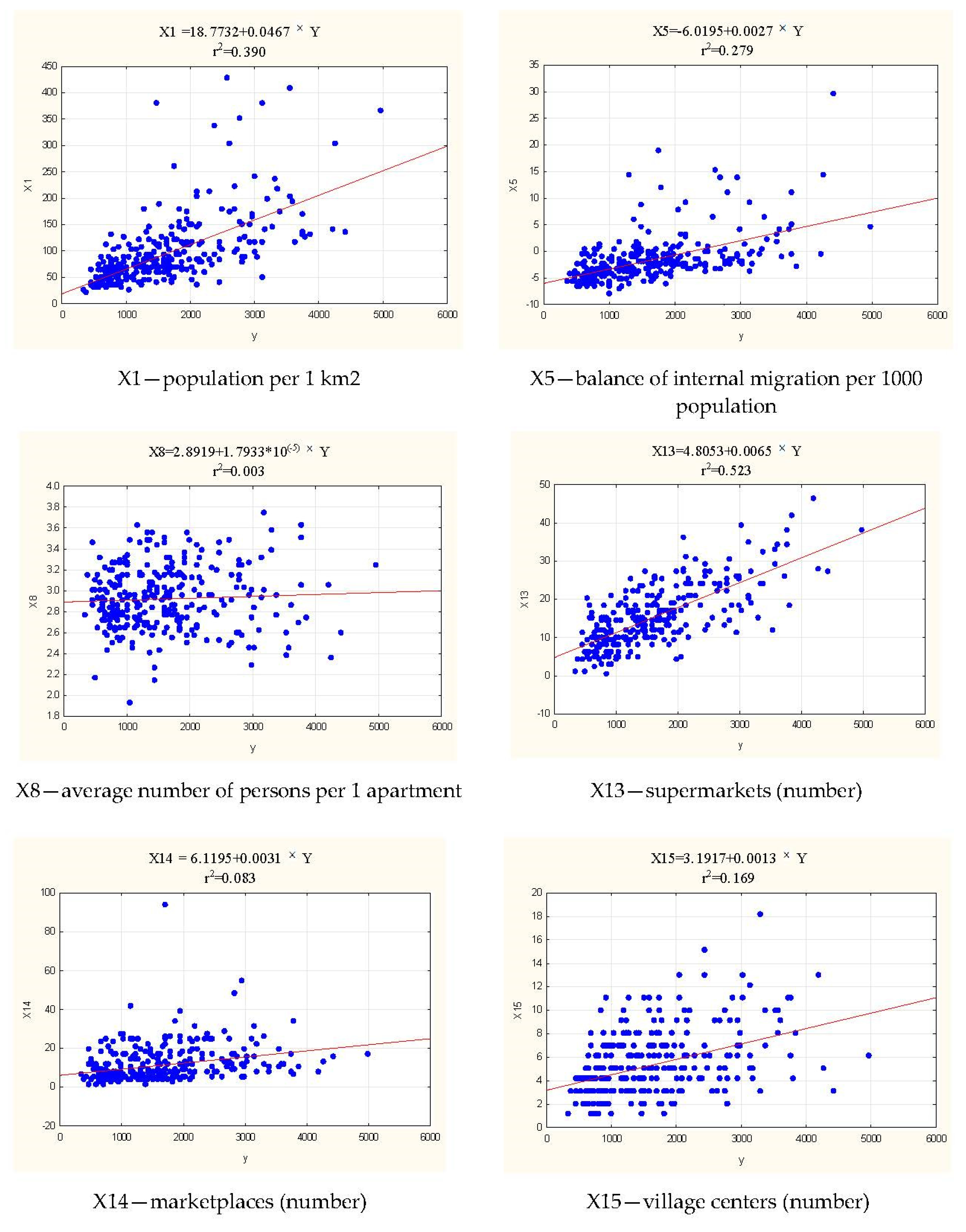
- If the value of the variable X13 (supermarkets (number)) increases by one unit, the value of the WO(pop) composite index increases by 0.0065.
- If the value of the variable X1 (population per 1 km2) increases by one unit, the value of the composite index WO(pop) increases by 0.0467 (Figure 11).
- If the value of the variable X5 (balance of internal migration per 1000 population) increases by one unit, the value of the composite WO(pop) index increases by 0.0027.
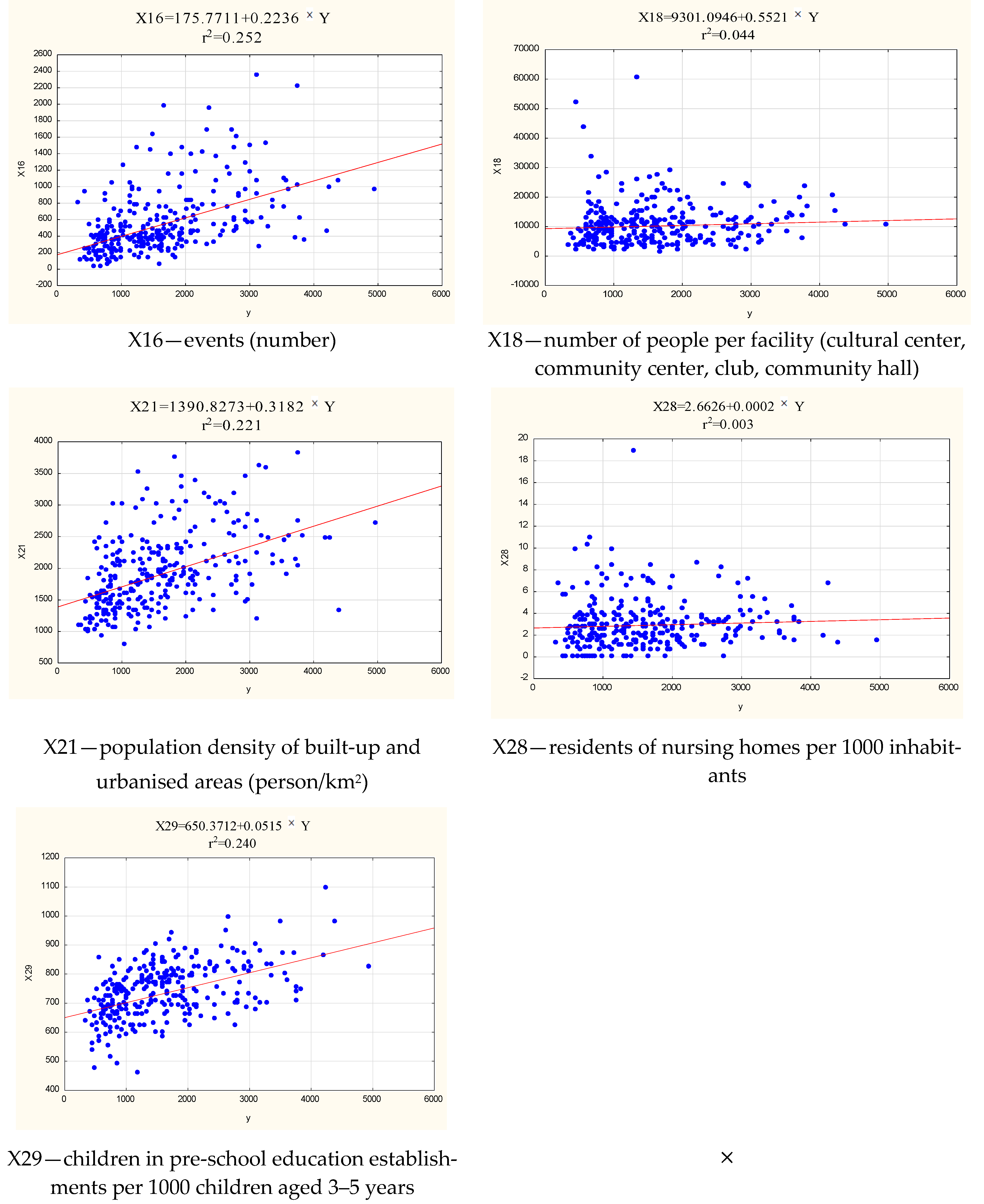
- If the value of the variable X16 (events (number)) increases by one unit, the value of the composite WO(pop) indicator will increase by 0.2236.
- If the value of the variable X21 (population density of built-up and urbanized areas (person/km2)) increases by one unit, the value of the composite WO(pop) index increases by 0.3182.
- If the value of the variable X29 (children in pre-school education establishments per 1000 children aged 3–5 years) increases by one unit, the value of the WO(pop) composite indicator will increase by 0.0515.
5. Conclusions
Limitations
Author Contributions
Funding
Institutional Review Board Statement
Informed Consent Statement
Data Availability Statement
Conflicts of Interest
References
- World Health Organization. Coronavirus Disease (COVID-2019) Situation Reports; World Health Organization: Geneva, Switzerland, 2019.
- Tyson, A. Republicans Remain Far Less Likely than Democrats to View COVID-19 as a Major Threat to Public Health; Pew Research Center: Washington, DC, USA, 2020. [Google Scholar]
- Rothgerber, H.; Wilson, T.; Whaley, D.; Rosenfeld, D.L.; Humphrey, M.; Moore, A.; Bihl, A. Politicizing the COVID-19 pandemic: Ideological differences in adherence to social distancing. PsyArXiv 2020. [Google Scholar] [CrossRef]
- Sirkeci, I.; Yucesahin, M.M. Coronavirus and Migration: Analysis of Human Mobility and the Spread of COVID-19. Migr. Lett. 2020, 17, 379–398. [Google Scholar] [CrossRef] [Green Version]
- Elleby, C.; Dominguez, I.P.; Adenauer, M.; Genovese, G. Impacts of the COVID-19 Pandemic on the Global Agricultural Markets. Environ. Resour. Econ. 2020, 76, 1067–1079. [Google Scholar] [CrossRef] [PubMed]
- Villulla, J.M. COVID-19 in Argentine agriculture: Global threats, local contradictions and possible responses. Agric. Hum. Values 2020, 37, 595–596. [Google Scholar] [CrossRef]
- Dev, S.M.; Sengupta, R. Covid-19: Impact on the Indian economy. In Indira Gandhi Institute of Development Research, Mumbai April; Indira Gandhi Institute of Development Research: Mumbai, India, 2020. [Google Scholar]
- Adekunle, I.A.; Onanuga, A.T.; Akinola, O.O.; Ogunbanjo, O.W. Modelling spatial variations of coronavirus disease (COVID-19) in Africa. Sci. Total Environ. 2020, 729, 138998. [Google Scholar] [CrossRef] [PubMed]
- Bartscher, A.K.; Nationalbank, D.; Seitz, S.; Siegloch, S.; Slotwinski, M.; Wehrhöfer, N. Social capital and the spread of Covid-19: Insights from European countries. J. Health Econ. 2021, 80, 102531. [Google Scholar] [CrossRef] [PubMed]
- Wright, A.L.; Sonin, K.; Driscoll, J.; Wilson, J. Poverty and economic dislocation reduce compliance with COVID-19 shelter-in-place protocols. J. Econ. Behav. Organ. 2020, 180, 544–554. [Google Scholar] [CrossRef]
- Franch-Pardo, I.; Napoletano, B.M.; Rosete-Verges, F.; Billa, L. Spatial analysis and GIS in the study of COVID-19. A review. Sci. Total Environ. 2020, 739, 140033. [Google Scholar] [CrossRef]
- Philip, R.N.; Bell, J.A.; Davis, D.J.; Beem, M.O.; Beigelman, P.M.; Engler, J.L.; Mellin, G.W.; Johnson, J.H.; Lerner, A.M. Epidemiologie Studies on Influenza in Familial and General Population Croups, 1951–1956. II Characteristics of Occurrence. Am. J. Hyg. 1961, 73, 123–137. [Google Scholar]
- Bouyer, J. Épidémiologie: Principes et Méthodes Quantitatives; Lavoisier: Paris, France, 2009. [Google Scholar]
- Cameron, D.; Jones, I.G. John Snow, the Broad Street pump and modern epidemiology. Int. J. Epidemiol. 1983, 12, 393–396. [Google Scholar] [CrossRef]
- Nyberg, F.; Pershagen, G. Epidemiologie studies on the health effects of ambient paniculate. Part Ambient Air A Health Risk Assess. 2000, 26, 49. [Google Scholar]
- Jończyk, J.A. Sytuacja Demograficzno-Epidemiologiczna a Zarządzanie Opieką Zdrowotną w Regionie: Studium Województwa Podlaskiego; Przedsiębiorczość I Zarządzanie: Warszawa, Poland, 2014; Volume 15. [Google Scholar]
- Ascani, A.; Faggian, A.; Montresor, S. The geography of COVID-19 and the structure of local economies: The case of Italy. J. Reg. Sci. 2021, 61, 407–441. [Google Scholar] [CrossRef]
- Velavan, T.P.; Meyer, C.G. The COVID-19 epidemic. Trop. Med. Int. Health 2020, 25, 278. [Google Scholar] [CrossRef] [Green Version]
- Folland, S. Does “community social capital” contribute to population health? Soc. Sci. Med. 2007, 64, 2342–2354. [Google Scholar] [CrossRef]
- Dobrzyński, M. Klimat organizacyjny jako regulator zachowania się ludzi. Organ. I Kier. 1981, 23. [Google Scholar]
- Borkowski, J. Podstawy Psychologii Spolecznej. Warszawa. (Basics of Social Psychology); ELIPSA Publishing House: Warsaw, Poland, 2003; pp. 37–67. [Google Scholar]
- Turowski, J. Socjologia: Małe Struktury Społeczne; Towarzystwo Naukowe Katolickiego Uniwersytetu Lubelskiego: Lublin, Poland, 2001. [Google Scholar]
- Znaniecki, F. Relacje Społeczne i Role Społeczne: Niedokończona Socjologia Systematyczna; Wydawnictwo Naukowe PWN: Warszawa, Poland, 2011. [Google Scholar]
- Adler, R.B.; Proctor, R.F.; Rosenfeld, L.B.; Skoczylas, G. Relacje Interpersonalne: Proces Porozumiewania Się; Dom Wydawniczy REBIS: Poznan, Poland, 2016. [Google Scholar]
- Mercer, A.J. Updating the epidemiological transition model. Epidemiol. Infect. 2018, 146, 680–687. [Google Scholar] [CrossRef] [Green Version]
- Badr, H.S.; Du, H.R.; Marshall, M.; Dong, E.S.; Squire, M.M.; Gardner, L.M. Association between mobility patterns and COVID-19 transmission in the USA: A mathematical modelling study. Lancet Infect. Dis. 2020, 20, 1247–1254. [Google Scholar] [CrossRef]
- Scheinkman, J.A. Social interactions. New Palgrave Dict. Econ. 2008, 2, 1–11. [Google Scholar]
- Gardner, W.; States, D.; Bagley, N. The Coronavirus and the Risks to the Elderly in Long-Term Care. J. Aging Soc. Policy 2020, 32, 310–315. [Google Scholar] [CrossRef] [Green Version]
- Jezierska-Thöle, A. Development of Rural Areas of Northern and Western Poland and Eastern Germany; Scientific Publishing House of the Nicolaus Copernicus University: Toruń, Poland, 2018. [Google Scholar]
- Mikhael, E.M.; Al-Jumaili, A.A. Can developing countries face novel coronavirus outbreak alone? The Iraqi situation. Public Health Pract. 2020, 1, 100004. [Google Scholar] [CrossRef]
- Tanne, J.H.; Hayasaki, E.; Zastrow, M.; Pulla, P.; Smith, P.; Rada, A.G. GLOBAL HEALTH Covid-19: How doctors and healthcare systems are tackling coronavirus worldwide. BMJ Br. Med. J. 2020, 368. [Google Scholar] [CrossRef] [Green Version]
- Stojkoski, V.; Utkovski, Z.; Jolakoski, P.; Tevdovski, D.; Kocarev, L. The socio-economic determinants of the coronavirus disease (COVID-19) pandemic. arXiv 2020, arXiv:2004.07947. [Google Scholar] [CrossRef]
- Kuebart, A.; Stabler, M. Infectious Diseases as Socio-Spatial Processes: The COVID-19 Outbreak in Germany. Tijdschr. Voor Econ. En Soc. Geogr. 2020, 111, 482–496. [Google Scholar] [CrossRef] [PubMed]
- Di Marco, M.; Baker, M.L.; Daszak, P.; De Barro, P.; Eskew, E.A.; Godde, C.M.; Harwood, T.D.; Herrero, M.; Hoskins, A.J.; Johnson, E.; et al. Sustainable development must account for pandemic risk. Proc. Natl. Acad. Sci. USA 2020, 117, 3888–3892. [Google Scholar] [CrossRef]
- Śleszyński, P.; Nowak, M.; Blaszke, M. Spatial policy in cities during the Covid-19 pandemic in Poland. TeMA-J. Land Use Mobil. Environ. 2020, 13, 427–444. [Google Scholar]
- Golinowska, S.; Zabdyr-Jamroz, M. Zarządzanie kryzysem zdrowotnym w pierwszym półroczu pandemii COVID-19. Analiza porównawcza na podstawie opinii ekspertów z wybranych krajów. Zesz. Nauk. Ochr. Zdrowia Zdr. Publiczne I Zarządzanie 2020, 18, 1–31. [Google Scholar] [CrossRef]
- Zahid, M.N.; Perna, S. Continent-wide analysis of COVID 19: Total cases, deaths, tests, socio-economic, and morbidity factors associated to the mortality rate, and forecasting analysis in 2020–2021. Int. J. Environ. Res. Public Health 2021, 18, 5350. [Google Scholar] [CrossRef]
- Manda, S.O.; Darikwa, T.; Nkwenika, T.; Bergquist, R. A Spatial Analysis of COVID-19 in African Countries: Evaluating the Effects of Socio-Economic Vulnerabilities and Neighbouring. Int. J. Environ. Res. Public Health 2021, 18, 10783. [Google Scholar] [CrossRef]
- Gwiazdzinska-Goraj, M.; Pawlewicz, K.; Jezierska-Thole, A. Differences in the Quantitative Demographic Potential-A Comparative Study of Polish-German and Polish-Lithuanian Transborder Regions. Sustainability 2020, 12, 9414. [Google Scholar] [CrossRef]
- Agnoletti, M.; Manganelli, S.; Piras, F. Covid-19 and rural landscape: The case of Italy. Landsc. Urban Plan. 2020, 204, 103955. [Google Scholar] [CrossRef]
- Laroze, D.; Neumayer, E.; Plumper, T. COVID-19 does not stop at open borders: Spatial contagion among local authority districts during England’s first wave. Soc. Sci. Med. 2021, 270, 113655. [Google Scholar] [CrossRef] [PubMed]
- Dutta, A.; Fischer, H.W. The local governance of COVID-19: Disease prevention and social security in rural India. World Dev. 2021, 138, 105234. [Google Scholar] [CrossRef] [PubMed]
- Sarwar, S.; Waheed, R.; Khan, A. COVID-19 challenges to Pakistan: Is GIS analysis useful to draw solutions? Sci. Total Environ. 2020, 730, 139089. [Google Scholar] [CrossRef] [PubMed]
- Wielechowski, M.; Czech, K.; Grzeda, L. Decline in Mobility: Public Transport in Poland in the time of the COVID-19 Pandemic. Economies 2020, 8, 78. [Google Scholar] [CrossRef]
- Ren, H.Y.; Zhao, L.; Zhang, A.; Song, L.Y.; Liao, Y.L.; Lu, W.L.; Cui, C. Early forecasting of the potential risk zones of COVID-19 in China’s megacities. Sci. Total Environ. 2020, 729, 138995. [Google Scholar] [CrossRef] [PubMed]
- Paul, A.; Englert, P.; Varga, M. Socio-economic disparities and COVID-19 in the USA. J. Phys. Complex. 2021, 2, 3. [Google Scholar] [CrossRef]
- Mollalo, A.; Vahedi, B.; Rivera, K.M. GIS-based spatial modeling of COVID-19 incidence rate in the continental United States. Sci. Total Environ. 2020, 728, 138884. [Google Scholar] [CrossRef]
- Kisielińska, J.; Stańko, S. Wielowymiarowa analiza danych w ekonomice rolnictwa. Rocz. Nauk Roln. Ser. G Ekon. Roln 2009, 96, 63–76. [Google Scholar]
- Sanchez-Zamora, P.; Gallardo-Cobos, R.; Cena-Delgado, F. Rural areas face the economic crisis: Analyzing the determinants of successful territorial dynamics. J. Rural Stud. 2014, 35, 11–25. [Google Scholar] [CrossRef]
- Dudzinska, M.; Bacior, S.; Prus, B. Considering the level of socio-economic development of rural areas in the context of infrastructural and traditional consolidations in Poland. Land Use Policy 2018, 79, 759–773. [Google Scholar] [CrossRef]
- Obilor, E.I.; Amadi, E.C. Test for significance of Pearson’s correlation coefficient. Int. J. Innov. Math. Stat. Energy Policies 2018, 6, 11–23. [Google Scholar]
- Gargiulo, C.; Gaglione, F.; Guida, C.; Papa, R.; Zucaro, F.; Carpentieri, G. The role of the urban settlement system in the spread of Covid-19 pandemic. The Italian case. TeMA-J. Land Use Mobil. Environ. 2020, 189–212. [Google Scholar]
- Prem, K.; Cook, A.R.; Jit, M. Projecting social contact matrices in 152 countries using contact surveys and demographic data. PLoS Comput. Biol. 2017, 13, e1005697. [Google Scholar] [CrossRef] [PubMed] [Green Version]
- Xu, Q.; Chraibi, M. On the effectiveness of the measures in supermarkets for reducing contact among customers during COVID-19 period. Sustainability 2020, 12, 9385. [Google Scholar] [CrossRef]
- Yezli, S.; Khan, A. COVID-19 social distancing in the Kingdom of Saudi Arabia: Bold measures in the face of political, economic, social and religious challenges. Travel Med. Infect. Dis. 2020, 37, 101692. [Google Scholar] [CrossRef]
- Salama, A.M. Coronavirus questions that will not go away: Interrogating urban and socio-spatial implications of COVID-19 measures. Emerald Open Res. 2020, 2, 14. [Google Scholar] [CrossRef] [Green Version]
- Pourghasemi, H.R.; Pouyan, S.; Heidari, B.; Farajzadeh, Z.; Shamsi, S.R.F.; Babaei, S.; Khosravi, R.; Etemadi, M.; Ghanbarian, G.; Farhadi, A. Spatial modeling, risk mapping, change detection, and outbreak trend analysis of coronavirus (COVID-19) in Iran (days between February 19 and June 14, 2020). Int. J. Infect. Dis. 2020, 98, 90–108. [Google Scholar] [CrossRef]
- Megahed, N.A.; Ghoneim, E.M. Antivirus-built environment: Lessons learned from Covid-19 pandemic. Sustain. Cities Soc. 2020, 61, 102350. [Google Scholar] [CrossRef]
- Mollalo, A.; Vahedi, B.; Bhattarai, S.; Hopkins, L.C.; Banik, S.; Vahedi, B. Predicting the hotspots of age-adjusted mortality rates of lower respiratory infection across the continental United States: Integration of GIS, spatial statistics and machine learning algorithms. Int. J. Med. Inform. 2020, 142, 104248. [Google Scholar] [CrossRef]
- Sugg, M.M.; Spaulding, T.J.; Lane, S.J.; Runkle, J.D.; Harden, S.R.; Hege, A.; Iyer, L.S. Mapping community-level determinants of COVID-19 transmission in nursing homes: A multi-scale approach. Sci. Total Environ. 2021, 752, 141946. [Google Scholar] [CrossRef]
- Yoosefi Lebni, J.; Abbas, J.; Moradi, F.; Salahshoor, M.R.; Chaboksavar, F.; Irandoost, S.F.; Nezhaddadgar, N.; Ziapour, A. How the COVID-19 pandemic effected economic, social, political, and cultural factors: A lesson from Iran. Int. J. Soc. Psychiatry 2021, 67, 298–300. [Google Scholar] [CrossRef] [PubMed]
- Bandura, R. A Survey of Composite Indices Measuring Country Performance: 2008 Update; United Nations Development Programme, Office of Development Studies (UNDP/ODS Working Paper): New York, NY, USA, 2008. [Google Scholar]
- Wu, C.; Barnes, D. A literature review of decision-making models and approaches for partner selection in agile supply chains. J. Purch. Supply Manag. 2011, 17, 256–274. [Google Scholar] [CrossRef]
- Prete, C.; Cozzi, M.; Viccaro, M.; Romano, S.; Ventura, G. Well-being and rurality: A spatial tool for rural development programs evaluation. Ital. Rev. Agric. Econ. 2017, 72, 267–287. [Google Scholar]
- Kocur-Bera, K.; Pszenny, A. Conversion of agricultural land for urbanization purposes: A case study of the suburbs of the capital of Warmia and Mazury, Poland. Remote Sens. 2020, 12, 2325. [Google Scholar] [CrossRef]
- Krzysztofik, R.; Kantor-Pietraga, I.; Runge, A.; Sporna, T. Is the Suburbanisation Stage Always Important in the Transformation of Large Urban Agglomerations? The Case of the Katowice Conurbation. Geogr. Pol. 2017, 90, 71–85. [Google Scholar] [CrossRef]
- Kaczorek, K. Wpływ pandemii COVID-19 na powrót polskiej kadry inżynierskiej z emigracji. Builder 2020, 276, 26–28. [Google Scholar] [CrossRef]
- Wspaniały, Ł. COVID-19: Liczba Chorych Bezobjawowych Jest Większa Niż Sądzono. Available online: https://www.uj.edu.pl/wiadomosci/-/journal_content/56_INSTANCE_d82lKZvhit4m/10172/145226636 (accessed on 3 March 2020).
- Parmet, W.E.; Sinha, M.S. Covid-19—The Law and Limits of Quarantine. N. Engl. J. Med. 2020, 382, e28. [Google Scholar] [CrossRef]
- Fu, Y.C.; Lee, H.W. Daily Contacts Under Quarantine amid Limited Spread of COVID-19 in Taiwan. Int. J. Sociol. 2020, 50, 434–444. [Google Scholar] [CrossRef]
- Alexander, D.; Karger, E. Do Stay-at-Home Orders Cause People to Stay at Home? Effects of Stay-at-Home Orders on Consumer Behavior; Working Paper Series WP 2020-12; Federal Reserve Bank of Chicago: Chicago, IL, USA, 2021. [Google Scholar]
- Abouk, R.; Heydari, B. The Immediate Effect of COVID-19 Policies on Social-Distancing Behavior in the United States. Public Health Rep. 2021, 136, 245–252. [Google Scholar] [CrossRef]
- Cronin, C.J.; Evans, W.N. Private precaution and public restrictions: What drives social distancing and industry foot traffic in the COVID-19 era? Natl. Bur. Econ. Res. 2020. Available online: http://www.nber.org/papers/w27531 (accessed on 9 March 2020).
- Zhou, P.; Yang, X.L.; Wang, X.G.; Hu, B.; Zhang, L.; Zhang, W.; Si, H.R.; Zhu, Y.; Li, B.; Huang, C.L.; et al. A pneumonia outbreak associated with a new coronavirus of probable bat origin. Nature 2020, 579, 270–273. [Google Scholar] [CrossRef] [PubMed] [Green Version]
- Andersen, K.G.; Rambaut, A.; Lipkin, W.I.; Holmes, E.C.; Garry, R.F. The proximal origin of SARS-CoV-2. Nat. Med. 2020, 26, 450–452. [Google Scholar] [CrossRef] [PubMed]
- Czech, K.; Karpio, A.; Wielechowski, M.W.; Woźniakowski, T.; Żebrowska-Suchodolska, D. Polska Gospodarka w Początkowym Okresie Pandemii COVID-19; Wydawnictwo SGGW: Warszawa, Poland, 2020. [Google Scholar]


| Factor | Social Interactions | |||||
|---|---|---|---|---|---|---|
| Nature of the Factors | Type of Interpersonal and Social Relations | |||||
| Md | Ms | Me | Isd | Ri | Ru | |
| Correlation Means Coefficients Significant with p < 0.500, n = 293 | ||||||
| 30 March 2020 | −0.298 | −0.126 | −0.165 | −0.292 | −0.109 | −0.315 |
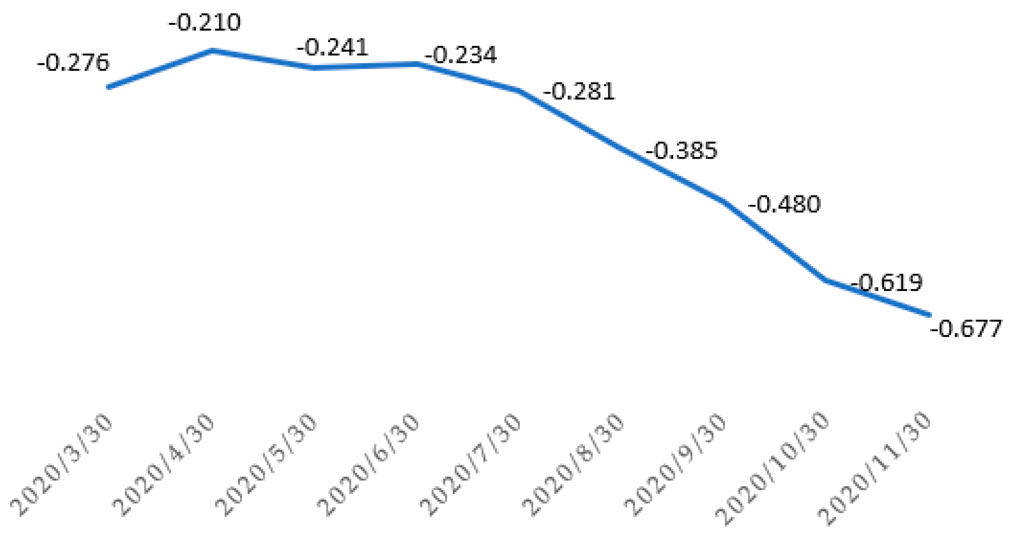
| 30 April 2020 | −0.176 | −0.091 | −0.163 | −0.180 | −0.046 | −0.241 |
| 30 May 2020 | −0.175 | −0.121 | −0.204 | −0.192 | −0.079 | −0.277 |
| 30 June 2020 | −0.171 | −0.094 | −0.196 | −0.177 | −0.098 | −0.270 |
| 30 July 2020 | −0.202 | −0.122 | −0.211 | −0.214 | −0.152 | −0.304 |
| 30 August 2020 | −0.286 | −0.170 | −0.257 | −0.301 | −0.224 | −0.401 |
| 30 September.2020 | −0.372 | −0.209 | −0.304 | −0.387 | −0.303 | −0.484 |
| 30 October 2020 | −0.454 | −0.256 | −0.413 | −0.472 | −0.386 | −0.607 |
| 30 November 2020 | −0.530 | −0.288 | −0.484 | −0.547 | −0.415 | −0.683 |
| Independent Variable | Coefficient b | Sdev. | t-Student | p | Nature of the Factors |
|---|---|---|---|---|---|
| X1—population per 1 km2 | 2.31 | 0.64 | 3.61 | 0.0004 | D (i,u) |
| X5—balance of internal migration per 1000 population | 43.12 | 6.92 | 6.23 | 0.0001 | D (i,u) |
| X8—average number of persons per 1 apartment | 416.43 | 96.55 | 4.31 | 0.0001 | S (i) |
| X13—supermarkets (number) | 40.30 | 4.22 | 9.55 | 0.0001 | E (u) |
| X14—marketplaces (number) | 61.61 | 10.14 | 6.08 | 0.0001 | E (u) |
| X15—village centers (number) | 8.33 | 4.06 | 2.05 | 0.0412 | S (i) |
| X16—events (number) | 0.21 | 0.10 | 2.11 | 0.0360 | S (i) |
| X18—number of people per facility (cultural center, community center, club, community hall) | 0.01 | 0.001 | 2.03 | 0.0436 | S (i) |
| X21—population density of built-up and urbanised areas (person/km2) | 0.20 | 0.06 | 3.22 | 0.0014 | L (u) |
| X28—residents of nursing homes per 1000 inhabitants | 23.08 | 11.10 | 2.08 | 0.0385 | S (i) |
| X29—children in pre-school education establishments per 1000 children aged 3–5 years | 1.10 | 0.34 | 3.23 | 0.0014 | S (i) |
| constant | 810.33 | 354.02 | 2.90 | 0.0001 | |
| R | 0.880 | ||||
| Adjusted R2 | 0.766 | ||||
| Number of observations | 298 | ||||
| F(11,298) | 86.138 |
Publisher’s Note: MDPI stays neutral with regard to jurisdictional claims in published maps and institutional affiliations. |
© 2022 by the authors. Licensee MDPI, Basel, Switzerland. This article is an open access article distributed under the terms and conditions of the Creative Commons Attribution (CC BY) license (https://creativecommons.org/licenses/by/4.0/).
Share and Cite
Dudzińska, M.; Gwiaździńska-Goraj, M.; Jezierska-Thöle, A. Social Factors as Major Determinants of Rural Development Variation for Predicting Epidemic Vulnerability: A Lesson for the Future. Int. J. Environ. Res. Public Health 2022, 19, 13977. https://doi.org/10.3390/ijerph192113977
Dudzińska M, Gwiaździńska-Goraj M, Jezierska-Thöle A. Social Factors as Major Determinants of Rural Development Variation for Predicting Epidemic Vulnerability: A Lesson for the Future. International Journal of Environmental Research and Public Health. 2022; 19(21):13977. https://doi.org/10.3390/ijerph192113977
Chicago/Turabian StyleDudzińska, Małgorzata, Marta Gwiaździńska-Goraj, and Aleksandra Jezierska-Thöle. 2022. "Social Factors as Major Determinants of Rural Development Variation for Predicting Epidemic Vulnerability: A Lesson for the Future" International Journal of Environmental Research and Public Health 19, no. 21: 13977. https://doi.org/10.3390/ijerph192113977