Article

Factors Influencing O3 Concentration in Traffic and Urban Environments: A Case Study of Guangzhou City

1
College of Geographical Science, Harbin Normal University, Harbin 150025, China
2
Guangdong Open Laboratory of Geospatial Information Technology and Application, Lab of Guangdong for Utilization of Remote Sensing and Geographical Information System, Guangzhou Institute of Geography, Guangdong Academy of Sciences, Guangzhou 510070, China
3
Southern Marine Science and Engineering Guangdong Laboratory (Guangzhou), Guangzhou 511485, China
*
Authors to whom correspondence should be addressed.
These authors contributed equally to this work.
Int. J. Environ. Res. Public Health 2022, 19(19), 12961; https://doi.org/10.3390/ijerph191912961
Submission received: 26 August 2022 / Revised: 1 October 2022 / Accepted: 6 October 2022 / Published: 10 October 2022

Abstract

:
Ozone (O3) pollution is a serious issue in China, posing a significant threat to people’s health. Traffic emissions are the main pollutant source in urban areas. NOX and volatile organic compounds (VOCs) from traffic emissions are the main precursors of O3. Thus, it is crucial to investigate the relationship between traffic conditions and O3 pollution. This study focused on the potential relationship between O3 concentration and traffic conditions at a roadside and urban background in Guangzhou, one of the largest cities in China. The results demonstrated that no significant difference in the O3 concentration was observed between roadside and urban background environments. However, the O3 concentration was 2 to 3 times higher on sunny days (above 90 μg/m3) than on cloudy days due to meteorological conditions. The results confirmed that limiting traffic emissions may increase O3 concentrations in Guangzhou. Therefore, the focus should be on industrial, energy, and transportation emission mitigation and the influence of meteorological conditions to minimize O3 pollution. The results in this study provide some theoretical basis for mitigation emission policies in China.

1. Introduction

Air pollution has become a crucial issue in China due to rapid economic development [1]. The Chinese government has exerted a significant effort to reduce air pollution in recent years. As a result, fine particulate matter (PM2.5) has significantly decreased due to strict emission mitigation policies [2]. Ozone (O3) has become the most prevalent pollutant in China. The O3 concentration has increased by 10.6% from 2015 to 2021 in 339 [3,4]. Excessive exposure to O3 can be extremely harmful to human health, causing substantial damage and irritation to the eyes, respiratory tract, and lungs [5,6,7].
Many studies have focused on O3 pollution in China, investigating the spatiotemporal variations [8,9,10,11,12], secondary formation mechanism [13,14,15], emission sources [16,17,18,19], and other factors. The Pearl River Delta (PRD) is one of the most developed regions in China and has experienced significant O3 pollution. The O3 concentration has increased in the PRD since 2015 [20]. The O3 pollution is the highest in autumn in the PRD due to high temperatures, strong solar radiation, and low relative humidity (RH) [21,22,23,24,25]. In addition, several studies confirmed the “weekend effect” [26,27] in China, i.e., the O3 concentration is higher on weekends than during working days in Beijing [28], Shanghai [29,30], and Guangzhou [31]. There are two reasons. First, the nitric oxide (NO) concentration is lower during the weekend due to fewer traffic emissions. Therefore, the inhibitory effect of NO on O3 is weaker, and more O3 is generated. Second, fewer aerosol particles are emitted during the weekend, resulting in less scattering and absorption of solar radiation. As a result, more O3 is formed due to the stronger solar radiation during weekends [32].
There are three major sources of near-ground O3 precursors: traffic emissions [33], industry emissions, and emissions by power plants [34]. Mitigating O3 pollution has become a crucial issue in the PRD region in recent years [35]. However, it is challenging to control O3 pollution due to the complex O3 generation mechanism [36]. After absorbing ultraviolet light, tropospheric O2 decomposes into two O atoms. The O atoms are combined with O2 to form O3 (Equations (1) and (2)). In urban areas, NO2 in traffic emissions is the main precursor of O3 (Equation (3)). O3 rapidly oxidize NO to form NO2, known as the titration effect (Equation (4)).
O 2 + U V   O + O
O + O 2 + M     O 3 + M
N O 2 + h v     N O + O
O 3 + N O     N O 2 + O 2
In these processes, a dynamic equilibrium exists during the formation and consumption of O3 by NOX. However, alkoxy radicals (RO) and hydroperoxyl radicals (HO2) generated by the reaction of volatile organic compounds (VOCs) and hydroxyl (OH) radicals in the atmosphere also react with NO (Equations (5)–(8)), destroying the dynamic balance between NOX and O3 and increasing the O3 concentration.
H O 2 + N O     H O + N O 2
R O 2 + N O     R O + N O 2
H O + R H + O 2     R O 2 + H 2 O
R O + O 2 + h v     H O 2 + R C H O
If large amounts of NOX are emitted, HO and RO2 react predominantly with NO2 (Equations (9) and (10)); if small amounts of NOX are emitted, the free radical reaction dominates (Equations (11) and (12)). According to the formation mechanism of O3, the O3 concentration is closely related to the NOX and VOCs concentrations because of the highly nonlinear relationship between O3 and its precursors. Therefore, it is more difficult to mitigate O3 than other pollutants.
R O 2 + N O 2     R O 2 N O 2
H O + N O 2     H N O 3
H O 2 + H O 2     H 2 O 2 + O 2
H O 2 + R O 2     R O 2 H + O 2
The O3 concentration depends on the O3 formation process and diffusion [37,38,39]. Accordingly, the photochemical reaction rate [40], human activities, and meteorological conditions are the three dominant factors affecting the local O3 concentration [41,42]. Many studies have demonstrated that low cloudiness [43,44], intense solar radiation [45], high temperature [46,47], and low RH [48] can accelerate the O3 production rate [49,50]. High road network density [51], frequent motor vehicle braking, rapid acceleration, and high traffic flow [52] lead to high NOX emissions [53]. Wind speed and direction can affect the horizontal distribution of O3 in local areas, and a low wind speed facilitates O3 accumulation [54,55].
Traffic emissions are the main pollutant source in urban areas. NOX and VOC from traffic emissions are the main precursors of O3. Therefore, it is necessary to investigate the relationship between traffic conditions and O3 pollution. However, there are very few studies focusing on the influence of traffic situations on O3. We investigate the potential relationship between the O3 concentration and traffic conditions at roadside and urban background stations in Guangzhou, one of the largest cities in the PRD and China. The results provide a scientific reference for policymakers to establish emission mitigation policies.

2. Materials and Methods

2.1. Study Area and Measurement Data

Guangzhou is one of the largest cities in China, with a developed economy, dense population, and advanced manufacturing industries. The atmospheric pollutant concentrations were obtained from three national monitoring stations: two roadside stations (Yangji station (YJ station) and Huangsha station (HS station)) and one urban background station (Luhu station (LH station)) (Figure 1). The YJ station is located at an intersection of the main road (Zhongshan road) in the city center, about 5 m higher above ground. The HS station is located on a three-layer viaduct. The measurement instruments were installed between the second and third layers, about 20 m above the ground. The LH station is situated in Luhu Park, allowing us to compare air pollution in traffic and an urban park. The national measurement data were obtained from Guangzhou Ecological Environment Bureau (http://sthjj.gz.gov.cn/, accessed on 1 July 2021). The temporal resolution of the measurement data is one hour.
Meteorological data were obtained from Guangzhou Weather website (http://www.tqyb.com.cn/gz/weatherLive/autoStation/, accessed on 1 July 2021), including ambient temperature, wind speed, wind direction, solar radiation, and RH. The dynamic traffic data were obtained from the Guangzhou Municipal Bureau of Transportation (http://jtj.gz.gov.cn/jtcx/lkcx/, accessed on 1 July 2021). All the data were quality-controlled and covered the period from January to June 2021.

2.2. Analysis Approaches

A stepwise regression model was used to investigate the relationship between the potential impact factors and O3 concentration. Stepwise regression analysis automatically selects the most important variables to establish a predictive or explanatory model. The influencing factor are incorporated into the model one by one, and the statistical significance was evaluated. The insignificant factors were removed from the model.

3. Results and Discussion

3.1. Temporal Variations of NO2 and O3

3.1.1. Daily Variations

Generally, pollutant concentrations are affected by several factors, such as emission sources, meteorological conditions, and pollutant formation mechanisms. The median diurnal variation of O3 and NO2 during the cold (from January to March) and warm (from April to June) seasons is shown in Figure 2. Similar diurnal patterns of O3 are observed at the three stations. The O3 concentration is low from 22:00 to the early morning on the following day. Then, it rapidly increases from around 8:00 in the morning and reaches the maximum around 14:00–16:00. As the solar radiation increases during the daytime, the O3 concentration increases [56,57] (Equations (1) and (2)). However, the O3 concentration remains low during the night. There are two reasons. First, less O3 is generated in the absence of sunlight. Second, NO can react with O3 to form NO2 and O2 during the night (Equation (4)), which is referred to as the titration effect of NO.
The diurnal variation of NO2 differs from that of O3. As shown in Figure 2d–f, the NO2 concentration is lower at 3:00–4:00 and 12:00–16:00 and higher at 6:00–8:00 and 20:00–22:00. The highest NO2 concentration occurs at 20:00–22:00. The NO2 concentration shows an increasing trend from 04:00–8:00 at the two roadside stations (HS and JY) because of traffic emissions. This increasing trend is not observed at the urban background station (LH). The solar radiation increases after 08:00. NO2 reacts with VOCs to produce O3, resulting in a decreasing trend at all three stations. The NO2 concentration increases after 16:00 due to lower solar radiation and a decrease in the photochemical reaction [58,59,60]. During the night, the NO2 concentration increases again due to the titration effect [61].
The seasonal difference in the pollutant concentration is larger for NO2 than for O3, as shown in Figure 2d–f. The NO2 concentration is higher in the cold season (from January to March) than in the warm season (from April to June). The decisive factor influencing the seasonal variation of the NO2 concentration is solar radiation. The average solar radiance in Guangzhou is 1352 kJ/ m2 in the cold season and 1806 kJ/ m2 in the warm season. Lower solar radiation leads to less O3 generation and less NO2 consumption. Another possible factor may be the lower RH in winter. In Guangzhou, the average RH is 59.04% and 86.2% in the cold and warm seasons, respectively [62,63]. A higher RH results in a stronger photochemical reaction and a lower NO2 concentration in the warm season. Another possible explanation is the seasonal change in the planetary boundary layer height. It is 717 m in winter and 1239 m in summer in Guangzhou [64,65]. A lower planetary boundary layer accumulates NO2, resulting in a higher NO2 concentration [66]. However, the seasonal difference in the O3 concentration is smaller than that of the NO2 concentration. The reason is that O3 is a secondary pollutant whose concentration is controlled by highly complex and nonlinear secondary formation mechanisms.

3.1.2. Weekly Variations

The weekly variations in the O3 and NO2 concentrations at the three stations are illustrated in Figure 3. In general, the weekly trends of the O3 and NO2 concentrations are similar at three stations, but the average concentrations are different. As shown in Figure 3a, the O3 concentration is significantly higher on weekends (Saturday and Sunday) than on weekdays (from Monday to Friday), indicating the weekend effect of O3. It is believed to be related to a change in the proportion of O3 precursor emissions and other pollutant emissions from human activities [67]. Fewer human activities on weekends lead to lower PM2.5 and a lower aerosol optical thickness and radiation extinction. Therefore, the O3 concentrations are higher on the weekend than on weekdays due to stronger photochemical reactions [68,69]. Moreover, high traffic flow during the morning rush hour results in a rapid increase in the NO concentration, inhibiting O3 formation on weekdays [70,71].
Differences in the O3 concentration are observed at the three stations. The highest O3 concentration was measured at the LH station, followed by the two roadside stations YJ and HS. The reason is the surrounding environment. The LH station is located in Luhu Park. VOCs generated by biological sources compete with NO, reducing the inhibition of NO on O3 and leading to a higher O3 concentration [72,73]. The YJ station is surrounded mostly by business and entertainment areas with frequent human activities. Large amounts of NOX are emitted from traffic inhibited O3 formation. In addition, the titration effect of NO is stronger at the YJ station, leading to a slightly lower O3 concentration at the YJ station than at the LH station. The HS station is a roadside station located near a park. It has higher vegetation cover than the YJ station.
The weekly variation in the NO2 concentration shows a significantly different pattern than that of the O3 concentration. The NO2 concentration is slightly higher on weekdays than on the weekend due to higher anthropogenic emissions, especially traffic emissions in urban areas [74,75,76,77]. The NO2 concentration is the highest at the HS station, followed by the YJ and LH stations, which is consistent with the traffic emissions and the local environment of the three stations.

3.2. Influencing Factors

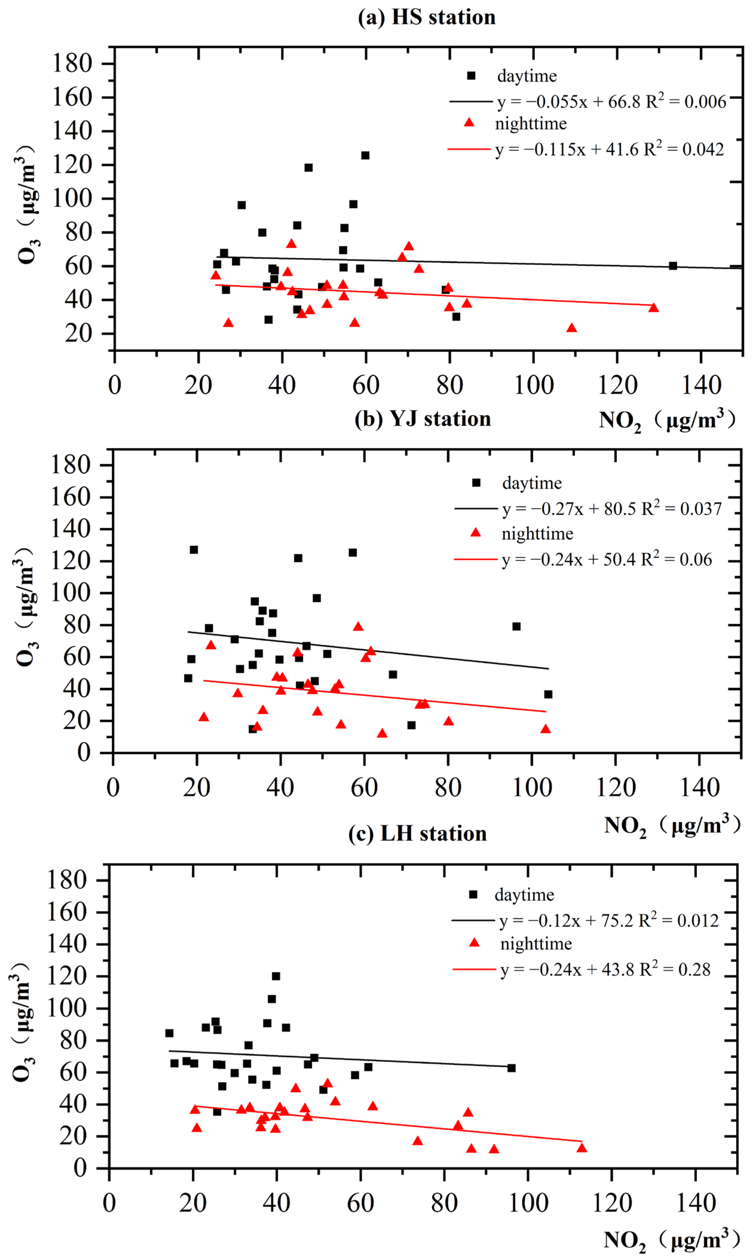
3.2.1. Synergistic Variation of O3 and NO2

Figure 4 shows the scatterplots of the O3 and NO2 concentrations during the daytime (07:00–19:00) and nighttime (20:00–06:00) at the three stations. The linear regression model has a negative slope for all three stations during the daytime and nighttime, indicating that the NO2 concentration decreases as the O3 concentration increases. However, differences are observed between daytime and nighttime. In the daytime, NO2 is consumed, and O3 is produced (Equations (2) and (3)). However, without a photochemical reaction during nighttime, O3 is converted to NO2 due to the titration effect (Equation (4)), leading to a lower O3 concentration. Due to the highly nonlinear and complex O3 formation mechanism, the R2 value is low for all fitting results. The R2 value is larger during nighttime at all three stations due to the absence of the photochemical reaction, the titration effect of NO, and weaker vertical diffusion [78,79]. The nighttime fitting degree is better at the LH station than at the roadside stations. The reason might be the surrounding environment of the LH station. The vegetation cover is higher; thus, vegetation respiration is stronger at night. Consequently, the NO2 and O3 concentrations are relatively stable, leading to a better fitting degree.
The fitted results of the three stations are similar. However, the dominant emission sources differ at the three stations. This result indicates no significant effect of traffic emissions on the O3 concentration at the roadside stations. Due to the absence of VOCs, a dynamic equilibrium exists between O3 and NOX in the atmosphere. Thus, O3 is not accumulated and does not exceed the air pollution standard [80,81]. However, the reaction between VOCs and NO weakens the inhibitory effect of NO on O3, resulting in high O3 pollution [82]. Controlling NOX emissions does not mitigate O3 pollution. Moreover, Guangzhou is in the VOC-limitation area [83,84]. Limiting vehicle emissions to reduce the NOX concentration may even increase the O3 concentration. Therefore, the focus should be on industrial, energy, and transportation emission mitigation and the influence of meteorological conditions to minimize O3 pollution.

3.2.2. Pearson Correlation and Stepwise Regression Analyses
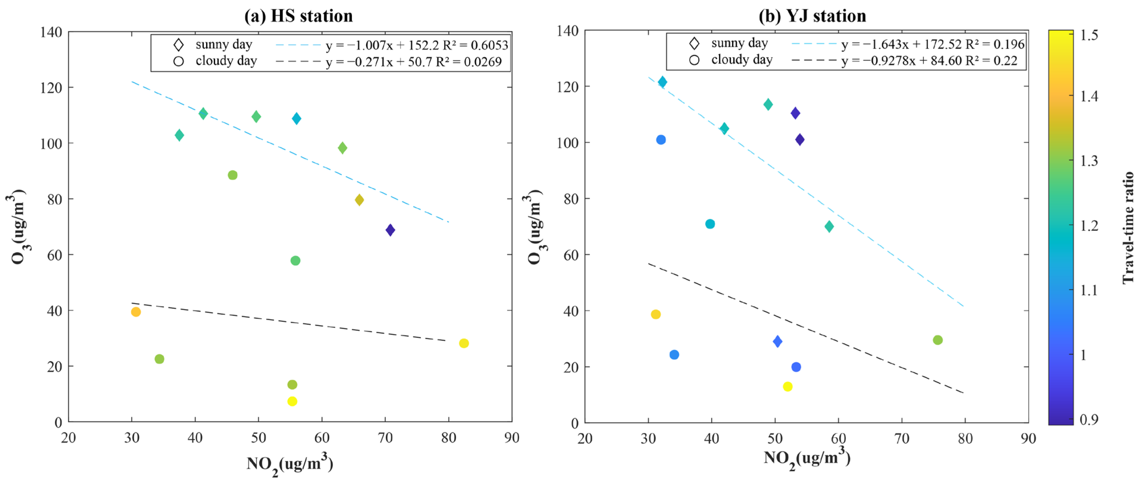
Pearson correlation analysis and stepwise regression analysis were conducted to describe the relationship between the pollutant concentration and other factors, such as meteorological parameters and dynamic traffic parameters. Table 1 and Table 2 show the results of Pearson’s correlation analysis and stepwise regression analysis, respectively. Pearson’s correlation shows the correlation between the O3 concentration and potential factors, and the stepwise regression model determines the significant impact factors. The beta values are used to quantify the contribution of the variables. Briefly, the O3 concentration is positively correlated with solar radiation, temperature, and travel-time ratio and negatively correlated with the NO2 concentration, wind speed, and vehicle speed (Table 1). The stepwise regression model shows that the significant factors affecting O3 concentration are temperature, NO2 concentration, and RH. As shown in Table 1, the O3 concentration positively correlates with the travel-time ratio. The travel time ratio is the ratio of the actual travel time to the ideal travel time in smooth traffic flow. The larger the ratio, the higher the degree of traffic congestion. The NOX and VOC emissions are higher during frequent vehicle braking than during uniform driving. Thus, more O3 precursors are emitted, leading to a significant positive correlation between O3 concentration and travel-time ratio. The temperature is positively correlated with O3 concentration as a result of O3 formation. The negative correlation between the NO2 and O3 concentrations has already been discussed in Section 3.2.1. Moreover, a negative correlation is observed between vehicle speed and O3 concentration. The fuel consumption is higher at higher speeds than at lower speeds, resulting in more precursor emissions and a higher O3 concentration. Wind speed and O3 concentration are negatively correlated because of the dilution effect. The O3 concentration is lower at higher RH due to wet deposition. Moreover, an increase in RH significantly reduces the number of oxygen atoms, reducing the amount of O3 generation.
The secondary pollutant O3 is correlated with several factors. The vehicle speed and travel-time ratio are significantly correlated with the O3 concentration, indicating the importance of traffic emissions on O3 pollution in urban areas.

3.2.3. Case Study

As discussed in the previous section, traffic emissions affect the O3 concentration but are not the dominant factor. Many studies demonstrated that solar radiation was a significant factor influencing O3 formation. A case study was conducted to quantify the influence of solar radiation on O3 concentration in Guangzhou. Two weeks were selected: 1 February to 7 February 2021, with sunny weather, and 24 February to 2 March 2021, with cloudy weather.
The pollutant concentrations and related parameters are listed in Table 3. The O3 concentration is substantially different on sunny and cloudy days at all three stations, indicating the predominant influence of solar radiation. The O3 concentration is 2–3 times higher on sunny days than on cloudy days in the daytime and nighttime. However, there are no large differences in the NO2 concentration. In the daytime, there are no differences in the NO2 concentration between sunny and cloudy days. However, the nighttime NO2 concentration is 1.5 to 2 times higher on sunny days than on cloudy days. More O3 is formed during sunny days, leading to a stronger titration effect and a higher NO2 concentration during the nighttime on sunny days. It should be noted that the NO2 concentration is lower at the LH station than at the two roadside stations during the daytime. However, the O3 concentration is similar at all three stations due to the lower inhibitory effect of NO, as discussed in Section 3.1.2. This finding confirms our results, i.e., traffic emissions contribute significantly to O3 generation, but the contribution is not higher at roadside stations than at the urban background station.
The scatterplots of the NO2 and O3 concentrations in the two periods at YJ and HS are shown in Figure 5. The colored dots indicate the dynamic traffic conditions. The linear regression results demonstrate that the negative correlation between the NO2 and O3 concentrations is stronger during the daytime than during the nighttime at both stations due to the stronger photochemical reaction strength. Furthermore, no significant relationship is observed between the O3 concentration and dynamic traffic conditions.

4. Conclusions

This study evaluated the factors influencing the O3 concentration in traffic and urban background environments. The diurnal and weekly variation of the O3 and NO2 concentrations demonstrated a similar pattern at the three stations. These results were attributed to differences in the O3 generation mechanism, meteorological conditions, and emission sources. However, no significant differences in the O3 variation were observed between the three stations, implying that the O3 concentration was not significantly higher in the traffic environment than in the urban background environment. Since Guangzhou is located in a VOC-limited area, the lower O3 concentration in the urban background area is due to the lower inhibition of NO on O3.
Pearson correlation analysis and stepwise regression analysis were used to describe the relationship between the pollutant concentration and the influencing factors, such as meteorological and dynamic traffic parameters. Traffic and meteorological parameters (temperature, solar radiation, RH, and precipitation) were significantly correlated with the O3 concentration at the two roadside stations. It was concluded that traffic emissions contributed to O3 pollution in the urban area but were not the decisive factor, while the meteorological factors also influenced the O3 concentration.
A case study was conducted for two weeks to quantify the influence of solar radiation on O3 concentration in Guangzhou. On sunny days, the O3 concentration exceeded 90 μg/m3 at the three sites. It was 2 to 3 times higher than during cloudy days due to meteorological conditions. The dynamic traffic condition (travel-time ratio) had no significant relationship with the O3 and NO2 concentrations at the two roadside stations.
This study analyzed the temporal variation of O3 and its precursor NO2 at roadside and urban background environments in Guangzhou and its influencing factors. The results confirmed that limiting traffic emissions might increase O3 concentrations in Guangzhou. Therefore, emission mitigation should be performed, i.e., industrial, energy, and transportation emission mitigation, and the influence of meteorological conditions should be considered to minimize O3 pollution. However, some limitations exist in this study. Due to a lack of NO and VOCs data, the relationship between O3 concentration and NO and VOCs was not analyzed. In future, a mobile measurement focusing on O3 will be carried out in Guangzhou, and a more detailed analysis will be performed.

Author Contributions

Data analysis and writing of the original draft: T.L., J.S.; Concept construction and supervision: M.L., Y.D.; Data analysis, review, and editing, B.L., W.J. and J.Y. All authors have read and agreed to the published version of the manuscript.

Funding

This research was fund by the Key Special Project for Introduced Talents Team of Southern Marine Science and Engineering Guangdong Laboratory (Guangzhou), grant number GML2019ZD0301; National Natural Science Foundation of China, grant number 41901372 and 41976189; Science and Technology Program of Guangzhou, grant number 202002030247; the GDAS’ Project of Science and Technology Development, grant number 2022GDASZH-2022010202 and the Science and Technology Program of Guangdong, grant number 2021B1212100006.

Institutional Review Board Statement

Not applicable.

Informed Consent Statement

Not applicable.

Data Availability Statement

The data presented in this study are available on request from the corresponding website.

Acknowledgments

We would like to thank the anonymous reviewers for their constructive comments. We also thank the Geographical Science Data Center of The Greater Bay Area for providing the relevant data for this study.

Conflicts of Interest

The authors declare no conflict of interest.

References

  1. Zheng, Y.; Peng, J.; Xiao, J.; Su, P.; Li, S. Industrial structure transformation and provincial heterogeneity characteristics evolution of air pollution: Evidence of a threshold effect from China. Atmos. Pollut. Res. 2020, 11, 598–609. [Google Scholar] [CrossRef]
  2. He, Q.; Zhang, M.; Song, Y.; Huang, B. Spatiotemporal assessment of PM2.5 concentrations and exposure in China from 2013 to 2017 using satellite-derived data. J. Clean. Prod. 2021, 286, 124965. [Google Scholar] [CrossRef]
  3. Liu, D.; Li, J.; Su, X.; Zuo, R. Analysis of ozone sources in Xining based on CAMx-OSAT method. J. Environ. Sci. 2021, 41, 386–394. [Google Scholar]
  4. Alfoldy, B.; Kotb, M.; Yigiterhan, O.; Safi, M.A.; Giamberini, S. BTEX, nitrogen oxides, ammonia and ozone concentrations at traffic influenced and background urban sites in an arid environment. Atmos. Pollut. Res. 2018, 10, 445–454. [Google Scholar] [CrossRef]
  5. Wang, X.; Zhao, W.; Li, L.; Yang, X.; Jiang, J.; Sun, S. Spatial and temporal distribution characteristics of ozone in China and its influence on socio-economic factors. Earth Environ. 2020, 48, 66–75. [Google Scholar]
  6. Lin, H.; An, Q.; Chao, L.; Pun, V.C.; Chi, S.C.; Tian, L. Gaseous air pollution and acute myocardial infarction mortality in Hong Kong: A time-stratified case-crossover study. Atmos. Environ. 2013, 76, 68–73. [Google Scholar] [CrossRef]
  7. Cacciottolo, M.; Wang, X.; Driscoll, I.; Woodward, N.; Saffari, A.; Reyes, J.; Serre, M.L.; Vizuete, W.; Sioutas, C.; Morgan, T.E. Particulate air pollutants, APOE alleles and their contributions to cognitive impairment in older women and to amyloidogenesis in experimental models. Transl. Psychiatry 2017, 7, e1022. [Google Scholar] [CrossRef]
  8. Parrish, D.D.; Petropavlovskikh, I.; Oltmans, S.J. Reversal of Long-Term Trend in Baseline Ozone Concentrations at the North American West Coast. Geophys. Res. Lett. 2017, 44, 10,675–10,681. [Google Scholar] [CrossRef]
  9. Young, P.J.; Naik, V.; Fiore, A.M.; Gaudel, A.; Lewis, A. Tropospheric ozone assessment report: Assessment of global-scale model performance for global and regional ozone distributions, variability, and trends. Elem. Sci. Anthr. 2018, 6, 10. [Google Scholar]
  10. Tarasick, D.; Galbally, I.E.; Cooper, O.R.; Schultz, M.G.; Neu, J.L. Tropospheric ozone assessment report: Tropospheric ozone from 1877 to 2016, observed levels, trends and uncertainties. Elem. Sci. Anthr. 2019, 7, 39. [Google Scholar]
  11. Zhang, R.; Lei, W.; Tie, X.; Hess, P. Industrial emissions cause extreme urban ozone diurnal variability. Proc. Natl. Acad. Sci. USA 2004, 101, 6346–6350. [Google Scholar] [CrossRef] [PubMed] [Green Version]
  12. Zhang, Y.; Shao, K.; Tang, X.; Li, J. Studies on photochemical smog pollution in Chinese cities. J. Peking Univ. (Nat. Sci. Ed.) 1998, Z1, 260–268. [Google Scholar]
  13. Ma, W.; Feng, Z.; Zhan, J.; Liu, Y.; Liu, P.; Liu, C.; Ma, Q.; Yang, K.; Wang, Y.; He, H. Influence of photochemical loss of volatile organic compounds on understanding ozone formation mechanism. Atmos. Chem. Phys. 2022, 22, 4841–4851. [Google Scholar] [CrossRef]
  14. Liu, J.; Li, X.; Tan, Z.; Wang, W.; Zhang, Y. Assessing the Ratios of Formaldehyde and Glyoxal to NO2 as Indicators of O3–NOX –VOC sensitivity. Environ. Sci. Technol. 2021, 55, 10935–10945. [Google Scholar] [CrossRef] [PubMed]
  15. Zhang, K.; Huang, L.; Li, Q.; Huo, J.; Duan, Y.; Wang, Y.; Yaluk, E.; Wang, Y.; Fu, Q.; Li, L. Explicit modeling of isoprene chemical processing in polluted air masses in suburban areas of the Yangtze River Delta region: Radical cycling and formation of ozone and formaldehyde. Atmos. Chem. Phys. 2021, 21, 5905–5917. [Google Scholar] [CrossRef]
  16. Ge, S.; Wang, S.; Xu, Q.; Ho, T. Characterization and sensitivity analysis on ozone pollution over the Beaumont-Port Arthur Area in Texas of USA through source apportionment technologies. Atmos. Res. 2020, 247, 105249. [Google Scholar] [CrossRef]
  17. Liu, Y.; Song, M.; Liu, X.; Zhang, Y.; Hui, L.; Kong, L.; Zhang, Y.; Zhang, C.; Qu, Y.; An, J.; et al. Characterization and sources of volatile organic compounds (VOCs) and their related changes during ozone pollution days in 2016 in Beijing, China. Environ. Pollut. 2020, 257, 113599. [Google Scholar] [CrossRef]
  18. Wang, H.; An, J.; Shen, L.; Zhu, B.; Pan, C.; Liu, Z.; Liu, X.; Duan, Q.; Liu, X.; Wang, Y. Mechanism for the formation and microphysical characteristics of submicron aerosol during heavy haze pollution episode in the Yangtze River Delta, China. Sci. Total Environ. 2014, 490, 501–508. [Google Scholar] [CrossRef]
  19. Shen, L.; Wang, H.; Zhu, B.; Zhao, T.; Wang, Y. Impact of urbanization on air quality in the Yangtze River Delta during the COVID-19 lockdown in China. J. Clean. Prod. 2021, 296, 126561. [Google Scholar] [CrossRef]
  20. Xiao, L.; Hong, J.; Lin, Z.; Cooper, O.R.; Schultz, M.G.; Xu, X.; Tao, W.; Gao, M.; Zhao, Y.; Zhang, Y. Severe surface ozone pollution in China: A global perspective. Environ. Sci. Technol. 2018, 5, 487–494. [Google Scholar]
  21. Ma, S.; Shao, M.; Zhang, Y.; Dai, Q.; Xie, M. Sensitivity of PM2.5 and O3 pollution episodes to meteorological factors over the North China Plain. Sci. Total Environ. 2021, 792, 148474. [Google Scholar] [CrossRef] [PubMed]
  22. Liu, J.; Wang, L.; Li, M.; Liao, Z.; Kulmala, M. Quantifying the impact of synoptic circulations on ozone variations in North China from April–October 2013–2017. Atmos. Chem. Phys. 2019, 19, 14477–14492. [Google Scholar] [CrossRef] [Green Version]
  23. Liu, N.; Lin, W.; Ma, J.; Xu, W.; Xu, X. Seasonal variation in surface ozone and its regional characteristics at global atmosphere watch stations in China. J. Environ. Sci. 2019, 77, 291–302. [Google Scholar] [CrossRef] [PubMed]
  24. Li, M.; Yao, Y.; Luo, D.; Zhong, L. The Linkage of the Large-Scale Circulation Pattern to a Long-Lived Heatwave over Mideastern China in 2018. Atmosphere 2019, 10, 89. [Google Scholar] [CrossRef] [Green Version]
  25. Mao, J.; Wang, L.; Lu, C.; Liu, J.; Wang, Y. Meteorological mechanism for a large-scale persistent severe ozone pollution event over eastern China in 2017. J. Environ. Sci. 2020, 92, 187–199. [Google Scholar] [CrossRef]
  26. Sicard, P.; Paoletti, E.; Agathokleous, E.; Araminien, V.; Marco, A.D. Ozone weekend effect in cities: Deep insights for urban air pollution control. Environ. Res. 2020, in press. [CrossRef]
  27. Liu, H.; Deng, Y.; Huang, F.; Zhang, T.; Chen, Y. A study on the characteristics of ozone weekend effect and reaction sensitivity in Chengdu. IOP Conf. Ser. Earth Environ. Sci. 2020, 467, 012160. [Google Scholar] [CrossRef] [Green Version]
  28. Xza, B.; Wzb, C.; Lh, B. Human activities and urban air pollution in Chinese mega city: An insight of ozone weekend effect in Beijing. Phys. Chem. Earth Parts A/B/C 2019, 110, 109–116. [Google Scholar]
  29. Tang, W.; Zhao, C.; Geng, F.; Peng, L.; Zhou, G.; Gao, W.; Xu, J.; Tie, X. Study of ozone “weekend effect” in Shanghai. Sci. China (Ser. D Earth Sci.) 2008, 51, 1354–1360. [Google Scholar] [CrossRef]
  30. Wang, S.; Zhao, Y.; Han, Y.; Li, R.; Fu, H.; Gao, S.; Duan, Y.; Zhang, L.; Chen, J. Spatiotemporal variation, source and secondary transformation potential of volatile organic compounds (VOCs) during the winter days in Shanghai, China. Atmos. Environ. 2022, 286, 119203. [Google Scholar] [CrossRef]
  31. Zou, Y.; Charlesworth, E.; Yin, C.Q.; Yan, X.L.; Deng, X.J.; Li, F. The weekday/weekend ozone differences induced by the emissions change during summer and autumn in Guangzhou, China. Atmos. Environ. 2019, 199, 114–126. [Google Scholar] [CrossRef]
  32. Minschwaner, K.; Salawitch, R.; McElroy, M. Absorption of solar radiation by O2: Implications for O3 and lifetimes of N2O, CFCl3, and CF2Cl2. J. Geophys. Res. Atmos. 1993, 98, 10543–10561. [Google Scholar] [CrossRef]
  33. Bao, J.; Cao, J.; Gao, R.; Ren, Y.; Bi, F.; Wu, Z.; Chai, F.; Li, H. The prevention and control process, experience and enlightenment of ozone pollution in European ambient air to China. Environ. Sci. Res. 2021, 34, 890–901. [Google Scholar]
  34. Sun, X.; Zhang, H.; Yao, Y.; Zhou, W.; Ouyang, Z.; Wang, X. Applicability of atmospheric ozone passive monitoring methods and correlation analysis of influencing factors. Environ. Chem. 2021, 40, 2747–2754. [Google Scholar]
  35. Li, A.; Zhou, Q.; Xu, Q. Prospects for ozone pollution control in China: An epidemiological perspective. Environ. Pollut. 2021, 285, 117670. [Google Scholar] [CrossRef] [PubMed]
  36. Monks, P.S.; Archibald, A.; Colette, A.; Cooper, O.; Coyle, M.; Derwent, R.; Fowler, D.; Granier, C.; Law, K.S.; Mills, G. Tropospheric ozone and its precursors from the urban to the global scale from air quality to short-lived climate forcer. Atmos. Chem. Phys. 2015, 15, 8889–8973. [Google Scholar]
  37. Shen, J.; Huang, X.; Wang, Y.; Ye, S.; Pan, Y.; Chen, D.; Chen, H.; Qu, Y.; Lu, X.; Wang, Z. Characteristics and source analysis of ozone pollution in Guangdong Province. J. Environ. Sci. 2017, 37, 4449–4457. [Google Scholar]
  38. Jia, H.; Yin, T.; Qu, X.; Cheng, N.; Cheng, B.; Wang, J.; Tang, W.; Meng, F.; Chai, F. Characteristics and source simulation of ozone concentration in Beijing and surrounding areas in 2015. Environ. Sci. China 2017, 37, 1231–1238. [Google Scholar]
  39. Huang, Z.; Hong, L.; Yin, P.; Wang, X.; Zhang, Y. Study on the source of summer ozone pollution and the influence of atmospheric transport in Baoding. J. Peking Univ. (Nat. Sci. Ed.) 2018, 54, 665–672. [Google Scholar]
  40. Ling, Z.; Guo, H.; Lam, S.; Saunders, S.; Wang, T. Atmospheric photochemical reactivity and ozone production at two sites in Hong Kong: Application of a master chemical mechanism–photochemical box model. J. Geophys. Res. Atmos. 2014, 119, 10567–10582. [Google Scholar] [CrossRef]
  41. Cao, T.; Wu, K.; Kang, A.; Wen, X.; Li, H.; Wang, Y.; Lu, X.; Li, A.; Pan, W.; Fan, W. Analysis of ozone pollution characteristics and influencing factors in Chengdu-Chongqing urban agglomeration. J. Environ. Sci. 2018, 38, 1275–1284. [Google Scholar]
  42. Dainius, J.; Vaida, V.; Renata, C.I.; Milda, P.I. Surface ozone concentration and its relationship with UV Radiation, Meteorological Parameters and Radon on the Eastern Coast of the Baltic Sea. Atmosphere 2016, 7, 27. [Google Scholar]
  43. Deroubaix, A.; Brasseur, G.; Gaubert, B.; Labuhn, I.; Menut, L.; Siour, G.; Tuccella, P. Response of surface ozone concentration to emission reduction and meteorology during the COVID-19 lockdown in Europe. Meteorol. Appl. 2021, 28, e1990. [Google Scholar] [CrossRef]
  44. Juráň, S.; Šigut, L.; Holub, P.; Fares, S.; Klem, K.; Grace, J.; Urban, O. Ozone flux and ozone deposition in a mountain spruce forest are modulated by sky conditions. Sci. Total Environ. 2019, 672, 296–304. [Google Scholar] [CrossRef] [PubMed]
  45. Qi, J.; Mo, Z.; Yuan, B.; Huang, S.; Huangfu, Y.; Wang, Z.; Li, X.; Yang, S.; Wang, W.; Zhao, Y. An observation approach in evaluation of ozone production to precursor changes during the COVID-19 lockdown. Atmos. Environ. 2021, 262, 118618. [Google Scholar] [CrossRef] [PubMed]
  46. Abdullah, S.; Nasir, N.H.A.; Ismail, M.; Ahmed, A.N.; Jarkoni, M.N.K. Development of ozone prediction model in urban area. Int. J. Innov. Technol. Explor. Eng. 2019, 8, 2263–2267. [Google Scholar] [CrossRef]
  47. Wang, H.; Tan, Y.; Zhang, L.; Shen, L.; Zhao, T.; Dai, Q.; Guan, T.; Ke, Y.; Li, X. Characteristics of air quality in different climatic zones of China during the COVID-19 lockdown. Atmos. Pollut. Res. 2021, 12, 101247. [Google Scholar] [CrossRef]
  48. Dang, R.; Liao, H.; Fu, Y. Quantifying the anthropogenic and meteorological influences on summertime surface ozone in China over 2012–2017. Sci. Total Environ. 2021, 754, 142394. [Google Scholar] [CrossRef] [PubMed]
  49. Yu, Z.; Ma, J.; Mao, Z.; Cao, Y.; Qu, Y.; Xu, J. Analysis of meteorological conditions and weather classification of ozone pollution in Shanghai in 2017. J. Meteorol. Environ. 2019, 35, 46–54. [Google Scholar] [CrossRef]
  50. Zhao, W.; Fan, S.; Guo, H.; Gao, B.; Sun, J.; Chen, L. Assessing the impact of local meteorological variables on surface ozone in Hong Kong during 2000–2015 using quantile and multiple line regression models. Atmos. Environ. 2016, 144, 182–193. [Google Scholar] [CrossRef]
  51. Zhou, M.; Jiang, W.; Gao, W.; Zhou, B.; Liao, X. A high spatiotemporal resolution anthropogenic VOC emission inventory for Qingdao City in 2016 and its ozone formation potential analysis. Process Saf. Environ. Prot. 2020, 139, 147–160. [Google Scholar] [CrossRef]
  52. Balzotti, C.; Briani, M.; De Filippo, B.; Piccoli, B. A computational modular approach to evaluate mahram NO2 emissions and ozone production due to vehicular traffic. Discret. Contin. Dyn. Syst.-B 2022, 27, 3455. [Google Scholar] [CrossRef]
  53. Zhang, H.; Han, L.; Ren, Y.; Yao, Y.; Sun, X.; Wang, X.; Zhou, W.; Hua, Z. Monitoring of the gradient movement of surface ozone concentration in urban and northwestern suburbs of Beijing. Ecology 2019, 39, 6803–6815. [Google Scholar]
  54. Jing, S.; Ye, X.; Gao, Y.; Peng, Y.; Li, Y.; Wang, Q.; Shen, J.; Wang, H. The pollution characteristics and reactivity of volatile organic compounds during typical photochemical pollution in Hangzhou. Environ. Sci. 2020, 41, 3076–3084. [Google Scholar]
  55. Botlaguduru, V.S.; Kommalapati, R.R.; Huque, Z. Long-term meteorologically independent trend analysis of ozone air quality at an urban site in the greater Houston area. J. Air Waste Manag. Assoc. 2018, 68, 1051–1064. [Google Scholar] [CrossRef] [PubMed]
  56. Chen, W.; Chen, Y.; Chu, Y.; Zhang, J.; Xi, C.; Lin, C.; Feng, Z.; Lu, X. Numerical Simulation of Ozone Source Characteristics in the Pearl River Delta Region. J. Environ. Sci. 2022, 42, 293–308. [Google Scholar]
  57. Qin, Y.; Liu, M.; Song, J.; Yu, R.; Li, L.; Su, J. The temporal and spatial variation characteristics of near-surface O3 concentration in Guangdong-Hong Kong-Macao Greater Bay Area. J. Environ. Sci. 2021, 41, 2987–3000. [Google Scholar]
  58. Atkinson, R. Atmospheric chemistry of VOCs and NOx. Atmos. Environ. 2000, 34, 2063–2101. [Google Scholar] [CrossRef]
  59. Wang, T.; Xue, L.; Brimblecombe, P.; Lam, Y.F.; Li, L.; Zhang, L. Ozone pollution in China: A review of concentrations, meteorological influences, chemical precursors, and effects. Sci. Total Environ. 2016, 575, 1582–1596. [Google Scholar] [CrossRef] [PubMed]
  60. Chen, T.; Xue, L.; Zheng, P.; Zhang, Y.; Wang, W. Volatile organic compounds and ozone air pollution in an oil production region in northern China. Atmos. Chem. Phys. 2020, 20, 7069–7086. [Google Scholar] [CrossRef]
  61. Xiaomeng, J.; Arlene, F.; Folkert, B.K.; De, S.I.; Lukas, V. Inferring Changes in Summertime Surface Ozone-NOX-VOC Chemistry over U.S. Urban Areas from Two Decades of Satellite and Ground-Based Observations. Environ. Sci. Technol. 2021, 54, 6518–6529. [Google Scholar]
  62. Liu, C.; Peng, R.; Du, X.; Zhang, Y.; Luo, X. Comparative research of meteorological conditions of typical dense fog and haze process over Pearl River Delta region. Ecol. Environ. Sci. 2019, 28, 1818–1828. [Google Scholar]
  63. Yan, X.Y.; Hou, X.H.; Yang, Q.; Zhao, W.; Xu, Q.; Liu, Y.L. The variety of ozone and its relationship with meteorological conditions in typical cities in China. Plateau Meteorol. 2020, 39, 416–430. [Google Scholar]
  64. Huang, J.; Liao, B.T.; Shen, Z.Q.; Zhang, Z.J.; Lan, J.; Wang, C.L. Research and application of boundary layer height based on microwave radiometer and aerosol lidar. J. Trop. Meteorol. 2022, 38, 180–192. [Google Scholar]
  65. Song, L.; Deng, T.; Li, Z.L.; Wu, S.; He, G.W.; Li, F.; Wu, M.; Wu, D. Retrieval of boundary layer height and its influence on PM2.5 concentration based on lidar observation over Guangzhou. J. Trop. Meteorol. Engl. Ed. 2021, 27, 303–318. [Google Scholar]
  66. Levi, Y.; Dayan, U.; Levy, I.; Broday, D.M. On the association between characteristics of the atmospheric boundary layer and air pollution concentrations. Atmos. Res. 2020, 231, 104675. [Google Scholar]
  67. Monks, P.S. A review of the observations and origins of the spring ozone maximum. Atmos. Environ. 2000, 34, 3545–3561. [Google Scholar] [CrossRef]
  68. Yin, Y.; Shan, W.; Ji, X.; You, L.; Su, Y. Variation of atmospheric ozone concentration in Jinan. Environ. Sci. 2006, 34, 2299–2302. [Google Scholar]
  69. Pan, C.; Zhu, X.; Wang, J.; Feng, X.; Shen, Q.; Xia, W.; Wan, P.; Qiu, F. Characteristics and influencing factors of ozone pollution in Yunnan Province in 2019. Environ. Sci. Technol. 2020, 43, 156–164. [Google Scholar]
  70. Liu, Y.; Zhou, H.; Pei, Y.; Zhao, K.; Ren, Y. Characteristics of near-surface O3 concentrations in Harbin. J. Environ. Sci. 2018, 38, 4454–4463. [Google Scholar]
  71. Jenkin, M.E.; Clemitshawb, K.C. Ozone and other secondary photochemical pollutants: Chemical processes governing their formation in the planetary boundary layer. Atmos. Environ. 2000, 34, 2499–2527. [Google Scholar] [CrossRef]
  72. Lili, L.; Wang, L.; Liu, X.; Wang, K.; Xu, Y.; Li, S.; Jiang, J. Spatial-temporal distribution characteristics of ozone and the relationship between meteorological factors in Harbin. Environ. Sci. China 2020, 40, 1991–1999. [Google Scholar]
  73. Han, Z.; Zhang, M.; Hu, F. Numerical simulation of the effects of ecological NMHC on ozone and PAN. J. Environ. Sci. 2002, 3, 273–278. [Google Scholar]
  74. Kerimray, A.; Azbanbayev, E.; Kenessov, B.; Plotitsyn, P.; Alimbayeva, D.; Karaca, F. Spatiotemporal variations and contributing factors of air pollutants in almaty, Kazakhstan. Aerosol Air Qual. Res. 2020, 20, 1340–1352. [Google Scholar] [CrossRef] [Green Version]
  75. Carlsen, L.; Baimatova, N.; Kenessov, B.; Kenessova, O. Assessment of the Air Quality of Almaty. Focus. Traffic Compon. 2013, 5, 49–69. [Google Scholar]
  76. Wu, Y.; Zhang, S.; Hao, J.; Liu, H.; Wu, X.; Hu, J.; Walsh, M.P.; Wallington, T.J.; Zhang, K.M.; Stevanovic, S. On-road vehicle emissions and their control in China: A review and outlook. Sci. Total Environ. 2017, 574, 332–349. [Google Scholar] [CrossRef] [PubMed] [Green Version]
  77. Kerimray, A.; Bakdolotov, A.; Sarbassov, Y.; Inglezakis, V.; Poulopoulos, S. Air pollution in Astana: Analysis of recent trends and air quality monitoring system. Mater. Today Proc. 2018, 5, 22749–22758. [Google Scholar] [CrossRef]
  78. Chang, J.H.-W.; Griffith, S.M.; Lin, N.-H. Impacts of land-surface forcing on local meteorology and ozone concentrations in a heavily industrialized coastal urban area. Urban Clim. 2022, 45, 101257. [Google Scholar] [CrossRef]
  79. Wang, T.; Xue, L.; Feng, Z.; Dai, J.; Zhang, Y.; Tan, Y. Ground-level ozone pollution in China: A synthesis of recent findings on influencing factors and impacts. Environ. Res. Lett. 2022, 17, 063003. [Google Scholar] [CrossRef]
  80. Chameides, W.; Fehsenfeld, F.; Rodgers, M.; Cardelino, C.; Martinez, J.; Parrish, D.; Lonneman, W.; Lawson, D.; Rasmussen, R.; Zimmerman, P. Ozone precursor relationships in the ambient atmosphere. J. Geophys. Res. Atmos. 1992, 97, 6037–6055. [Google Scholar] [CrossRef]
  81. Tyagi, B.; Singh, J.; Beig, G. Seasonal progression of surface ozone and NOX concentrations over three tropical stations in North-East India. Environ. Pollut. 2020, 258, 113662. [Google Scholar] [CrossRef] [PubMed]
  82. Li, K.; Wang, H.; Chen, L.; Li, J.; Dong, F. Synergistic degradation of NO and C7H8 for inhibition of O3 generation. Appl. Catal. B Environ. 2022, 312, 121423. [Google Scholar] [CrossRef]
  83. Mao, J.; Yan, F.; Zheng, L.; You, Y.; Wang, W.; Jia, S.; Liao, W.; Wang, X.; Chen, W. Ozone control strategies for local formation-and regional transport-dominant scenarios in a manufacturing city in southern China. Sci. Total Environ. 2022, 813, 151883. [Google Scholar] [CrossRef] [PubMed]
  84. Wang, X.; Yin, S.; Zhang, R.; Yuan, M.; Ying, Q. Assessment of summertime O3 formation and the O3-NOX-VOC sensitivity in Zhengzhou, China using an observation-based model. Sci. Total Environ. 2022, 813, 152449. [Google Scholar] [CrossRef] [PubMed]
Figure 1. Overview of the study area and atmospheric monitoring stations. (a) Location of three stations; (b) Luhu station (LH); (c) Huangsha station (HS); (d) Yangji station (YJ).
Ijerph 19 12961 g001
Figure 2. Diurnal variation of typical pollutants in cold and warm seasons: O3 concentrations at (a) HS station, (b) YJ station, and (c) LH station; NO2 concentrations at (d) HS station, (e) YJ station, and (f) LH station.
Ijerph 19 12961 g002
Figure 3. Weekly variation in O3 (a) and NO2 (b) concentrations at the three stations.
Ijerph 19 12961 g003
Figure 4. Scatterplot of O3 and NO2 concentrations at HS (a), YJ (b), and LH (c).
Ijerph 19 12961 g004
Figure 5. Scatterplot of daily O3 and NO2 concentrations in the two periods at the HS (a) and YJ (b) stations. The colored dots denote the travel-time ratio.
Ijerph 19 12961 g005
Table 1. Pearson’s correlation coefficients between O3 concentration and various factors.
Impact FactorsDaytimeNighttime
Temperature (°C)0.047 **0.057 **
Wind speed (m/s)−0.082 **−0.057 **
Daily precipitation (mm)−0.101 **−0.006
Vehicle speed (m/s)−0.111 **−0.111 **
Travel-time ratio0.150 **0.129 **
NO2 (μg/m3)−0.220 *−0.153 **
RH (%)−0.495 **−0.226 **
Solar radiation (J/m2)0.448 **0.279 **
** Significant at the 0.01 level. * Significant at the 0.05 level.
Table 2. Results of stepwise regression model between O3 concentration and various factors.
ModelDaytimepNighttimep
Beta ValueBeta Value
Temperature (°C)0.3860.0000.2070.000
Wind speed (m/s)−0.0760.000−0.1240.000
Daily precipitation (mm)0.0920.0000.0360.037
Vehicle speed (m/s)−0.0770.000−0.0630.000
NO2 (μg/m3)−0.4070.000−0.6110.000
RH (%)−0.5780.000−0.3890.000
Solar radiation (J/m2)--0.1820.000
The dependent variable: O3 (μg/m3).
Table 3. The pollutant concentrations and related parameters in the two periods.
PeriodStationO3 (μg/m3)NO2 (μg/m3)Travel-Time RatioSolar Radiation (KJ/m2)RH (%)
Day TimeNight TimeDay TimeNight TimeDay TimeNight Time
Sunny daysHS97.4352.9554.2879.051.141.0317,627.0464.71%
JY94.7063.4548.8063.661.251.06
LH102.3145.8838.8779.34--
Cloudy daysHS37.3021.1552.3453.101.211.0510,300.8975.08%
JY42.9027.8646.1648.261.291.08
LH41.7025.7536.9941.59--
Publisher’s Note: MDPI stays neutral with regard to jurisdictional claims in published maps and institutional affiliations.

