
Urban–Rural Fringe Long-Term Sequence Monitoring Based on a Comparative Study on DMSP-OLS and NPP-VIIRS Nighttime Light Data: A Case Study of Shenyang, China

Abstract
:1. Introduction
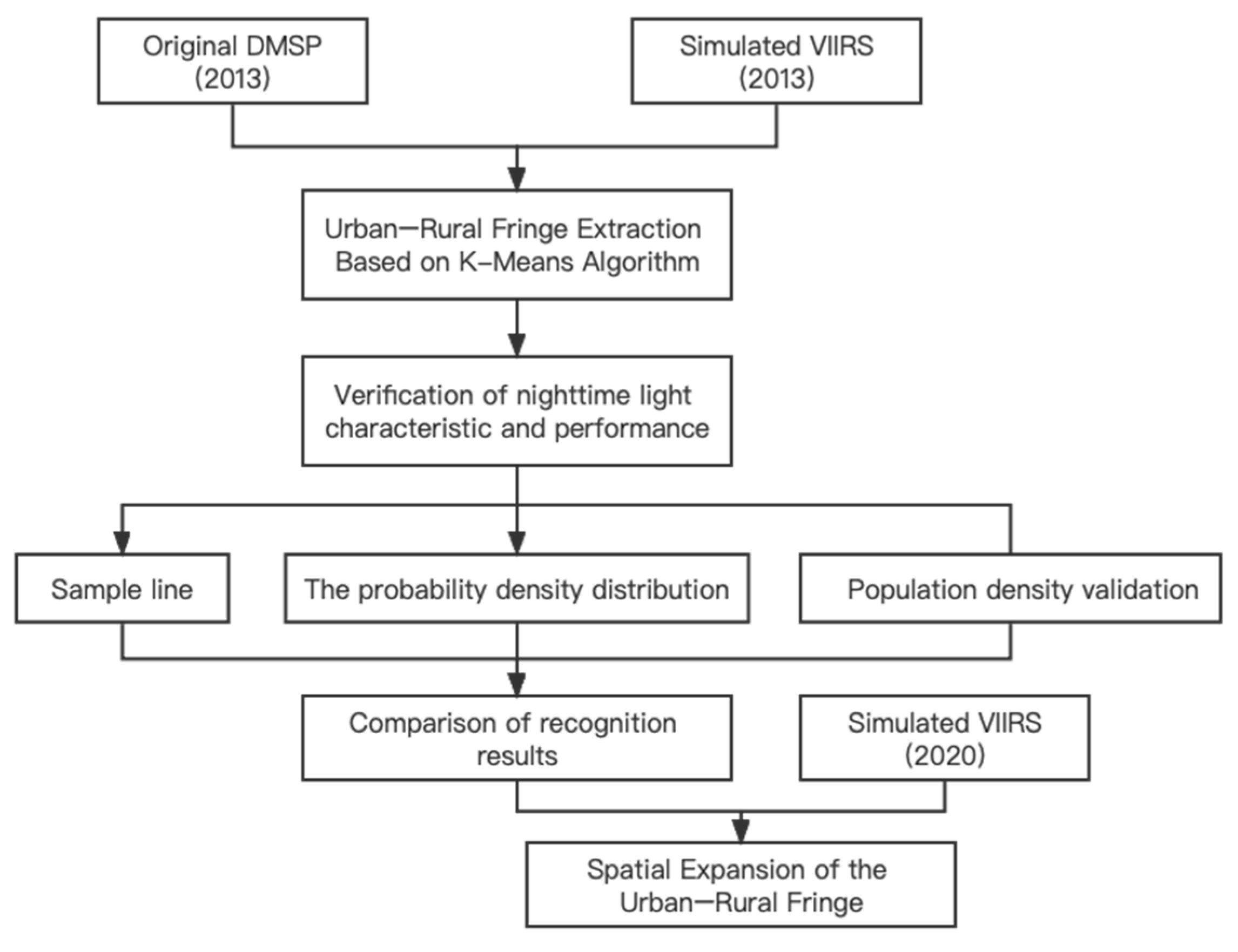
2. Methodology
2.1. Introduction to the Study Area
2.2. Materials
2.3. Urban–Rural Fringe Extraction Based on K-Means Algorithm
2.4. Verification of Nighttime Light Characteristics and Performance
- Sample line
- The probability density distribution
- Population density validation
3. Comparison of Recognition Results between DMSP Data and Transformed NPP Data in the SAME YEAR
3.1. Comparison of Nighttime Light Intensity and Light Fluctuation Characteristics
3.2. Performance Comparison Combining Nighttime Light Intensity and Light Fluctuation
3.3. Validation of Identification Results
4. Spatial Expansion of the Urban–Rural Fringe
4.1. Urban-Rural Fringe Expansion Analysis
4.2. Validation of Identification Results in 2020
5. Limitations and Research Perspectives
6. Conclusions
Author Contributions
Funding
Institutional Review Board Statement
Informed Consent Statement
Data Availability Statement
Conflicts of Interest
References
- Pryor, R.J. Defining the rural-urban fringe. Soc. Forces 1968, 47, 202–215. [Google Scholar] [CrossRef]
- Fu, C.; Chen, M. Research progress of urban and rural fringe in China. Prog. Geogr. 2010, 29, 1525–1531. [Google Scholar]
- Wang, X.; Shi, R.; Zhou, Y. Dynamics of urban sprawl and sustainable development in China. Socio-Econ. Plan. Sci. 2020, 70, 100736. [Google Scholar] [CrossRef]
- Kolbe, S.E.; Miller, A.I.; Cameron, G.N.; Culley, T.M. Effects of natural and anthropogenic environmental influences on tree community composition and structure in forests along an urban-wildland gradient in southwestern Ohio. Urban Ecosyst. 2016, 19, 915–938. [Google Scholar] [CrossRef]
- Yan, J.; Chen, H.; Xia, F. Toward improved land elements for urban–rural integration: A cell concept of an urban–rural mixed community. Habitat Int. 2018, 77, 110–120. [Google Scholar] [CrossRef]
- Dong, Q.; Qu, S.; Qin, J.; Yi, D.; Liu, Y.; Zhang, J. A Method to Identify Urban Fringe Area Based on the Industry Density of POI. ISPRS Int. J. Geo-Inf. 2022, 11, 128. [Google Scholar] [CrossRef]
- Sharp, J.S.; Clark, J.K. Between the country and the concrete: Rediscovering the rural–urban fringe. City Community 2008, 7, 61–79. [Google Scholar] [CrossRef]
- Chen, B. Review on identification method and driving mechanism of Peri-urban Area. Prog. Geogr. 2012, 31, 210–220. [Google Scholar]
- Xia, H. The Definition and Development Exploration of Shijiazhuang Urban Fringe; Hebei University: Baoding, China, 2008. [Google Scholar]
- Sylla, M.; Lasota, T.; Szewrański, S. Valuing Environmental Amenities in Peri-Urban Areas: Evidence from Poland. Sustainability 2019, 11, 570. [Google Scholar] [CrossRef]
- Zhou, Y.; Smith, S.J.; Elvidge, C.D.; Zhao, K. A cluster-based method to map urban area from DMSP/OLS nightlights. Remote Sens. Environ. 2014, 147, 173–185. [Google Scholar] [CrossRef]
- Yang, Y.; Ma, M.; Tan, C.; Li, W. Spatial recognition of the urban-rural fringe of Beijing using DMSP/OLS nighttime light data. Remote Sens. 2017, 9, 1141. [Google Scholar] [CrossRef]
- Li, X.; Li, D.; Xu, H.; Wu, C. Intercalibration between DMSP/OLS and VIIRS night-time light images to evaluate city light dynamics of Syria’s major human settlement during Syrian Civil War. Int. J. Remote Sens. 2017, 38, 5934–5951. [Google Scholar] [CrossRef]
- Bagan, H.; Yamagata, Y. Analysis of urban growth and estimating population density using satellite images of nighttime lights and land-use and population data. GISci. Remote Sens. 2015, 52, 765–780. [Google Scholar] [CrossRef]
- Dai, Z.; Hu, Y.; Zhao, G. The suitability of different nighttime light data for GDP estimation at different spatial scales and regional levels. Sustainability 2017, 9, 305. [Google Scholar] [CrossRef]
- Zheng, Q.; Weng, Q.; Wang, K. Characterizing urban land changes of 30 global megacities using nighttime light time series stacks. ISPRS J. Photogramm. Remote Sens. 2021, 173, 10–23. [Google Scholar] [CrossRef]
- Mustak, S.; Baghmar, N.K.; Srivastava, P.K.; Singh, S.K.; Binolakar, R. Delineation and classification of rural–urban fringe using geospatial technique and onboard DMSP–Operational Linescan System. Geocarto Int. 2018, 33, 375–396. [Google Scholar] [CrossRef]
- Duque, J.C.; Lozano-Gracia, N.; Patino, J.E.; Restrepo, P.; Velasquez, W.A. Spatiotemporal dynamics of urban growth in Latin American cities: An analysis using nighttime light imagery. Landsc. Urban Plan. 2019, 191, 103640. [Google Scholar] [CrossRef]
- Feng, Z.; Peng, J.; Wu, J. Using DMSP/OLS nighttime light data and K–means method to identify urban–rural fringe of megacities. Habitat Int. 2020, 103, 102227. [Google Scholar] [CrossRef]
- Chen, X.; Jia, X.; Pickering, M. Urban-Rural Fringe Recognition with the Integration of Optical and Nighttime Lights Data. In Proceedings of the IGARSS 2019–2019 IEEE International Geoscience and Remote Sensing Symposium, Yokohama, Japan, 28 July–2 August 2019; IEEE: Piscataway, NJ, USA, 2019; pp. 7435–7438. [Google Scholar]
- Peng, J.; Liu, Y.; Ma, J.; Zhao, S. A new approach for urban-rural fringe identification: Integrating impervious surface area and spatial continuous wavelet transform. Landsc. Urban Plan. 2018, 175, 72–79. [Google Scholar] [CrossRef]
- Elvidge, C.D.; Zhizhin, M.; Ghosh, T.; Hsu, F.C.; Taneja, J. Annual time series of global VIIRS nighttime lights derived from monthly averages: 2012 to 2019. Remote Sens. 2021, 13, 922. [Google Scholar] [CrossRef]
- Csatári, B.; Farkas, J.Z.; Lennert, J. Land use changes in the rural-urban fringe of Kecskemét after the economic transition. J. Settl. Spat. Plan. 2013, 4, 153–159. [Google Scholar]
- Han, M.; De Jong, M.; Cui, Z.; Xu, L.; Lu, H.; Sun, B. City branding in China’s northeastern region: How do cities reposition themselves when facing industrial decline and ecological modernization? Sustainability 2018, 10, 102. [Google Scholar] [CrossRef]
- Sun, H.; Li, X.; Guan, Y.; Tian, S.; Liu, H. The Evolution of the Urban Residential Space Structure and Driving Forces in the Megacity—A Case Study of Shenyang City. Land 2021, 10, 1081. [Google Scholar] [CrossRef]
- Feng, X.; Xiu, C.; Li, J.; Zhong, Y. Measuring the Evolution of Urban Resilience Based on the Exposure–Connectedness–Potential (ECP) Approach: A Case Study of Shenyang City, China. Land 2021, 10, 1305. [Google Scholar] [CrossRef]
- Version 4 DMSP-OLS Nighttime Lights Time Series and Version 2 NPP-VIIRS Nighttime Lights Time Series. Available online: https://eogdata.mines.edu/products/vnl/ (accessed on 12 March 2021).
- Elvidge, C.D.; Ziskin, D.; Baugh, K.E.; Tuttle, B.T.; Ghosh, T.; Pack, D.W.; Erwin, E.H.; Zhizhin, M. A fifteen year record of global natural gas flaring derived from satellite data. Energies 2009, 2, 595–622. [Google Scholar] [CrossRef]
- Liu, Z.; He, C.; Zhang, Q.; Huang, Q.; Yang, Y. Extracting the dynamics of urban expansion in China using DMSP-OLS nighttime light data from 1992 to 2008. Landsc. Urban Plan. 2012, 106, 62–72. [Google Scholar] [CrossRef]
- Wu, K.; Wang, X. Aligning pixel values of DMSP and VIIRS nighttime light images to evaluate urban dynamics. Remote Sens. 2019, 11, 1463. [Google Scholar] [CrossRef]
- Xu, R.; Wunsch, D. Survey of clustering algorithms. IEEE Trans. Neural Netw. 2005, 16, 645–678. [Google Scholar] [CrossRef]
- Jain, A.K.; Murty, M.N.; Flynn, P.J. Data clustering: A review. ACM Comput. Surv. CSUR 1999, 31, 264–323. [Google Scholar] [CrossRef]
- Delmelle, E.C. Five decades of neighborhood classifications and their transitions: A comparison of four US cities, 1970–2010. Appl. Geogr. 2015, 57, 1–11. [Google Scholar] [CrossRef]
- Zhang, G.; Zhang, C.; Zhang, H. Improved K-means algorithm based on density Canopy. Knowl.-Based Syst. 2018, 145, 289–297. [Google Scholar] [CrossRef]
- Thorn, J.; Thornton, T.F.; Helfgott, A. Autonomous adaptation to global environmental change in peri-urban settlements: Evidence of a growing culture of innovation and revitalisation in Mathare Valley Slums, Nairobi. Glob. Environ. Chang. 2015, 31, 121–131. [Google Scholar] [CrossRef]
- Vizzari, M.; Sigura, M. Landscape sequences along the urban–rural–natural gradient: A novel geospatial approach for identification and analysis. Landsc. Urban Plan. 2015, 140, 42–55. [Google Scholar] [CrossRef]
- Hu, S.; Tong, L.; Frazier, A.E.; Liu, Y. Urban boundary extraction and sprawl analysis using Landsat images: A case study in Wuhan, China. Habitat Int. 2015, 47, 183–195. [Google Scholar] [CrossRef]
- Liu, L.; Peng, Z.; Wu, H.; Jiao, H.; Yu, Y.; Zhao, J. Fast identification of urban sprawl based on K-means clustering with population density and local spatial entropy. Sustainability 2018, 10, 2683. [Google Scholar] [CrossRef]
- Ma, T.; Zhou, Y.; Zhou, C.; Haynie, S.; Pei, T.; Xu, T. Night-time light derived estimation of spatio-temporal characteristics of urbanization dynamics using DMSP/OLS satellite data. Remote Sens. Environ. 2015, 158, 453–464. [Google Scholar] [CrossRef]
- Steinley, D. K-means clustering: A half-century synthesis. Br. J. Math. Stat. Psychol. 2006, 59, 1–34. [Google Scholar] [CrossRef]
- Ahmad, A.; Dey, L. A k-mean clustering algorithm for mixed numeric and categorical data. Data Knowl. Eng. 2007, 63, 503–527. [Google Scholar] [CrossRef]
- Yang, D.; Xie, Z.; Du, X. Analysis of Land Cover Change in Shenyang Based on Remote Sensing Image Supervised Classification Technology. J. Phys. Conf. Ser. 2020, 1631, 012140. [Google Scholar] [CrossRef]
- Li, K.; Chen, Y. A Genetic Algorithm-based urban cluster automatic threshold method by combining VIIRS DNB, NDVI, and NDBI to monitor urbanization. Remote Sens. 2018, 10, 277. [Google Scholar] [CrossRef]
- Guo, W.; Lu, D.; Kuang, W. Improving fractional impervious surface mapping performance through combination of DMSP-OLS and MODIS NDVI data. Remote Sens. 2017, 9, 375. [Google Scholar] [CrossRef]
- Yue, H.; Liu, Y.; Li, Y.; Lu, Y. Eco-environmental quality assessment in China’s 35 major cities based on remote sensing ecological index. IEEE Access 2019, 7, 51295–51311. [Google Scholar] [CrossRef]
- Ye, M.; Yin, P.; Lee, W.C.; Lee, D.L. Exploiting geographical influence for collaborative point-of-interest recommendation. In Proceedings of the 34th international ACM SIGIR Conference on Research and Development in Information Retrieval, Beijing, China, 24–28 July 2011; pp. 325–334. [Google Scholar]
- Jiang, S.; Alves, A.; Rodrigues, F.; Ferreira, J., Jr.; Pereira, F.C. Mining point-of-interest data from social networks for urban land use classification and disaggregation. Comput. Environ. Urban Syst. 2015, 53, 36–46. [Google Scholar] [CrossRef] [Green Version]
- Wang, Y.; Gu, Y.; Dou, M.; Qiao, M. Using spatial semantics and interactions to identify urban functional regions. ISPRS Int. J. Geo-Inf. 2018, 7, 130. [Google Scholar] [CrossRef]
- Ramalho, C.E.; Hobbs, R.J. Time for a change: Dynamic urban ecology. Trends Ecol. Evol. 2012, 27, 179–188. [Google Scholar] [CrossRef] [PubMed]
- Shahrivari, S.; Jalili, S. Single-pass and linear-time K-means clustering based on MapReduce. Inf. Syst. 2016, 60, 1–12. [Google Scholar] [CrossRef]
- Xiong, C.; Hua, Z.; Lv, K.; Li, X. An Improved K-means text clustering algorithm By Optimizing initial cluster centers. In Proceedings of the 2016 7th International Conference on Cloud Computing and Big Data (CCBD), Macau, China, 16–18 November 2016; pp. 265–268. [Google Scholar]
- Flyvbjerg, B. Five misunderstandings about case-study research. Qual. Inq. 2006, 12, 219–245. [Google Scholar] [CrossRef] [Green Version]


| Source | DMSP/OLS | NPP/VIIRS |
|---|---|---|
| Spatial resolution | 1000 m | 500 m |
| Onboard calibration | No | Yes |
| Units of pixel values | Relative | Radiance (nanoWatts/(cm2 sr)) |
| Available temporal sequence | 1992–2013 annual composites | 2012–present monthly composites |
| Range of pixel values | 0–63 | 0–472.68 1 |
| Urban Area | Urban–Rural Fringe | Rural Area | ||||
|---|---|---|---|---|---|---|
| DMSP | VIIRS | DMSP | VIIRS | DMSP | VIIRS | |
| Min DN | 29.00 | 33.01 | 7.99 | 3.31 | 0.00 | 0.00 |
| Max DN | 63.00 | 63.00 | 60.78 | 62.54 | 28.23 | 21.37 |
| Mean DN | 59.11 | 59.56 | 28.82 | 24.94 | 6.45 | 3.42 |
| Standard deviation of DN | 5.67 | 6.25 | 10.59 | 9.64 | 5.09 | 3.86 |
| Min FI | 0.00 | 0.00 | 1.11 | 2.61 | 0.00 | 0.00 |
| Max FI | 46.00 | 40.67 | 46.00 | 40.67 | 46.00 | 40.07 |
| Mean FI | 8.09 | 7.50 | 20.27 | 16.69 | 4.63 | 4.20 |
| Standard deviation of FI | 9.31 | 9.75 | 8.83 | 7.72 | 4.16 | 3.84 |
| Urban Area | Urban–Rural Fringe | Rural Area | ||||
|---|---|---|---|---|---|---|
| DMSP | VIIRS | DMSP | VIIRS | DMSP | VIIRS | |
| Area (km2) | 1257 | 1399 | 1433 | 1872 | 9111 | 8339 |
| Light Intensity | High | Middle | Low | |||
| Light Fluctuation | Low | High | Low | |||
| Combination Characteristic | High–Low | Middle–High | Low–Low | |||
| Urban Area | Urban–Rural Fringe | Rural Area | ||||
|---|---|---|---|---|---|---|
| 2013 | 2020 | 2013 | 2020 | 2013 | 2020 | |
| Area (km2) | 1399 | 1762 | 1872 | 2537 | 8339 | 7502 |
| Min DN | 33.01 | 37.72 | 3.31 | 5.06 | 0.00 | 0.00 |
| Max DN | 63.00 | 63.00 | 62.54 | 63.00 | 21.37 | 25.70 |
| Mean DN | 59.56 | 60.71 | 24.94 | 27.90 | 3.42 | 6.02 |
| Standard deviation of DN | 6.25 | 4.96 | 9.64 | 9.35 | 3.86 | 4.71 |
| Min FI | 0.00 | 0.00 | 2.61 | 1.48 | 0.00 | 0.00 |
| Max FI | 40.67 | 43.75 | 40.67 | 43.75 | 40.07 | 43.75 |
| Mean FI | 7.50 | 5.30 | 16.69 | 15.15 | 4.20 | 6.02 |
| Standard deviation of FI | 9.75 | 8.29 | 7.72 | 7.90 | 3.84 | 4.14 |
Publisher’s Note: MDPI stays neutral with regard to jurisdictional claims in published maps and institutional affiliations. |
© 2022 by the authors. Licensee MDPI, Basel, Switzerland. This article is an open access article distributed under the terms and conditions of the Creative Commons Attribution (CC BY) license (https://creativecommons.org/licenses/by/4.0/).
Share and Cite
Zeng, T.; Jin, H.; Geng, Z.; Kang, Z.; Zhang, Z. Urban–Rural Fringe Long-Term Sequence Monitoring Based on a Comparative Study on DMSP-OLS and NPP-VIIRS Nighttime Light Data: A Case Study of Shenyang, China. Int. J. Environ. Res. Public Health 2022, 19, 11835. https://doi.org/10.3390/ijerph191811835
Zeng T, Jin H, Geng Z, Kang Z, Zhang Z. Urban–Rural Fringe Long-Term Sequence Monitoring Based on a Comparative Study on DMSP-OLS and NPP-VIIRS Nighttime Light Data: A Case Study of Shenyang, China. International Journal of Environmental Research and Public Health. 2022; 19(18):11835. https://doi.org/10.3390/ijerph191811835
Chicago/Turabian StyleZeng, Tianyi, Hong Jin, Zhifei Geng, Zihang Kang, and Zichen Zhang. 2022. "Urban–Rural Fringe Long-Term Sequence Monitoring Based on a Comparative Study on DMSP-OLS and NPP-VIIRS Nighttime Light Data: A Case Study of Shenyang, China" International Journal of Environmental Research and Public Health 19, no. 18: 11835. https://doi.org/10.3390/ijerph191811835