


Evaluation of Shallow Groundwater Quality at Regional Scales Using Adaptive Water Quality Indices
 , , , , and
Abstract
:1. Introduction
2. Materials and Methods
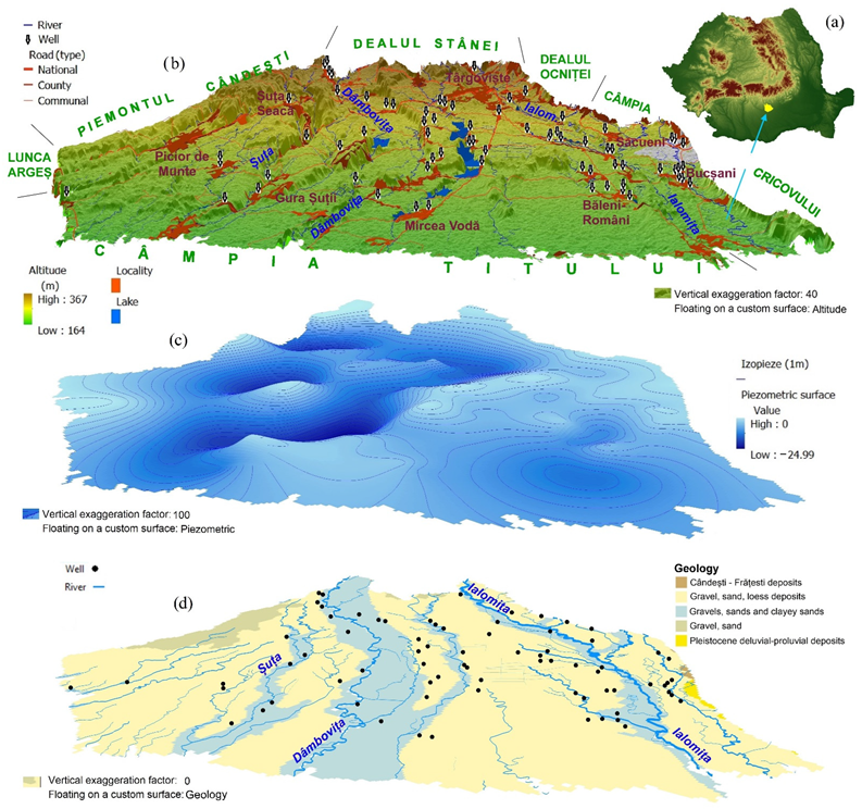
2.1. Study Area
2.2. Sampling and Analytical Procedures
2.3. Water Quality Index (WQI)
2.4. Integrated Weight Water Quality Index (IwWQI)
2.5. Data Interpolation and Hot-Spot Analysis
2.6. Assessment of the Impact on Human Health
3. Results
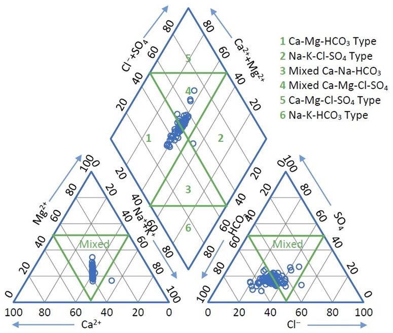
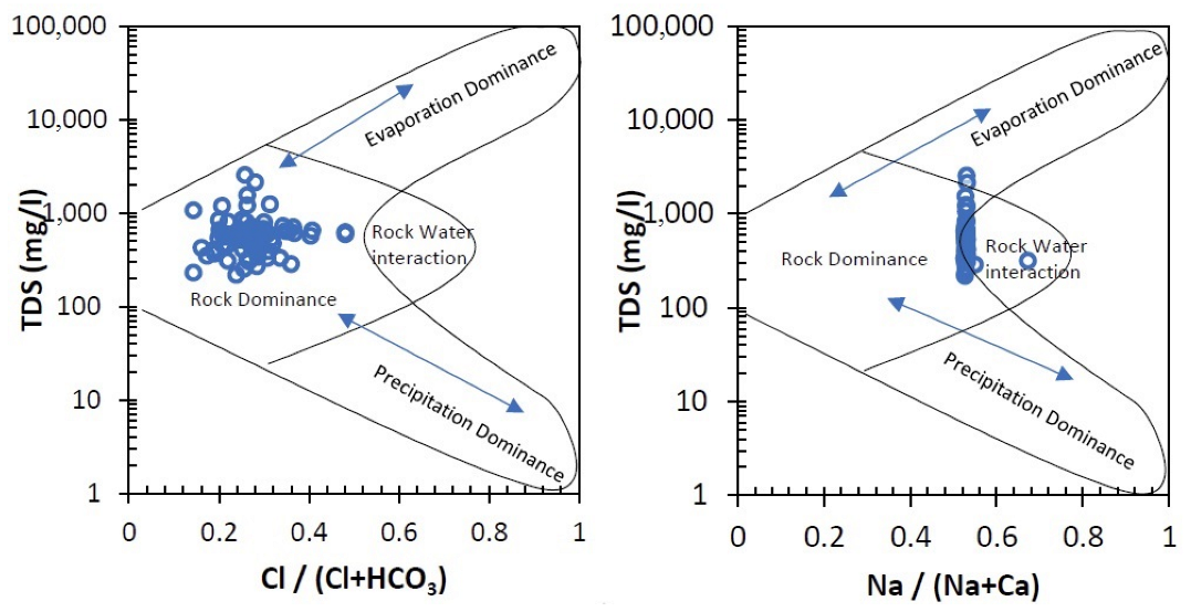
3.1. Hydrogeochemistry and Trace Element (TE) Evaluation
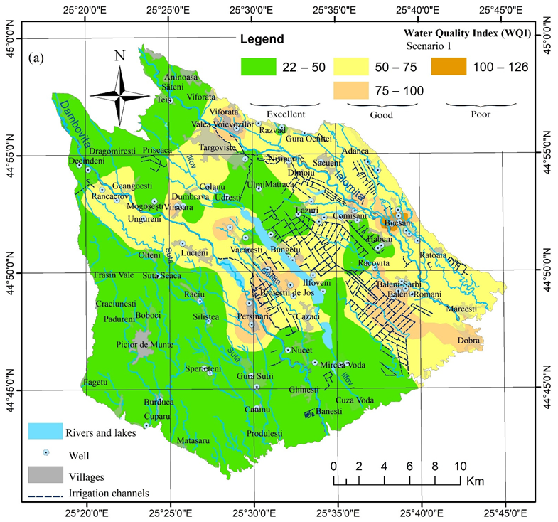
3.2. Water Quality for Human Consumption
3.3. Human Health Risk Assessments
4. Discussion
5. Conclusions
Author Contributions
Funding
Institutional Review Board Statement
Informed Consent Statement
Data Availability Statement
Conflicts of Interest
References
- Li, P.; Wu, J.; Qian, H.; Lyu, X.; Liu, H. Origin and assessment of groundwater pollution and associated health risk: A case study in an industrial park, northwest China. Environ. Geochem. Health 2014, 36, 693–712. [Google Scholar] [CrossRef] [PubMed]
- Jamorska, I.; Kubiak-Wójcicka, K.; Krawiec, A. Dynamics of the status of groundwater in the Polish Lowland: The River Gwda catchment example. Geologos 2019, 25, 193–204. [Google Scholar] [CrossRef]
- Rao, N.S.; Sunitha, B.; Adimalla, N.; Chaudhary, M. Quality criteria for groundwater use from a rural part of Wanaparthy District, Telangana State, India, through ionic spatial distribution (ISD), entropy water quality index (EWQI) and principal component analysis (PCA). Environ. Geochem. Health 2020, 42, 579–599. [Google Scholar]
- Lapworth, D.J.; Boving, T.B.; Kreamer, D.K.; Kebede, S.; Smedley, P.L. Groundwater quality: Global threats, opportunities and Realising the potential of groundwater. Sci. Total Environ. 2021, 811, 152471. [Google Scholar] [CrossRef]
- Angelakιs, A.N.; Zaccaria, D.; Krasilnikoff, J.; Salgot, M.; Bazza, M.; Roccaro, P.; Jimenez, B.; Kumar, A.; Yinghua, W.; Baba, A.; et al. Irrigation of World Agricultural Lands: Evolution through the Millennia. Water 2020, 12, 1285. [Google Scholar] [CrossRef]
- Zektser, I.S.; Everett, L.G. Groundwater Resources of the World and Their Use; UNESCO: Paris, France, 2004. [Google Scholar]
- Chakraborti, D.; Das, B.; Murrill, M.T. Examining India’s groundwater quality management. Env. Sci Technol. 2011, 45, 27–33. [Google Scholar] [CrossRef]
- Radulescu, C.; Bretcan, P.; Pohoata, A.; Tanislav, D.; Stirbescu, R.M. Assessment of drinking water quality using statistical analysis: A Case Study. Rom. J. Phys. 2016, 61, 1604–1616. [Google Scholar]
- Gonet, S.; Markiewicz, M.; Marszelewski, W.; Dziamski, A. Soil transformations in catchment of disappearing Sumówko Lake (Brodnickie Lake District, Poland). Limnol. Rev. 2010, 10, 133–137. [Google Scholar] [CrossRef]
- Rzymski, P.; Drewek, A.; Klimaszyk, P. Pharmaceutical pollution of aquatic environment: An emerging and enormous challenge. Limnol. Rev. 2017, 17, 97–107. [Google Scholar] [CrossRef]
- Xiang, J.; Zhou, J.J.; Yang, J.C.; Huang, M.H.; Feng, W.; Li, Q.Q.; Xue, D.X.; Zhao, Y.; Zhu, G.F. Applying multivariate statistics for identification of groundwater chemistry and qualities in the Sugan Lake Basin, Northern Qinghai-Tibet Plateau, China. J. Mt. Sci. 2020, 17, 448–463. [Google Scholar] [CrossRef]
- Snousy, M.G.; Wu, J.; Su, F.; Abdelhalim, A.; Ismail, E. Groundwater Quality and Its Regulating Geochemical Processes in Assiut Province, Egypt. Expo. Health 2021, 14, 305–323. [Google Scholar] [CrossRef]
- Mas-Pla, J.; Menció, A. Groundwater nitrate pollution and climate change: Learnings from a water balance-based analysis of several aquifers in a western Mediterranean region (Catalonia). Environ. Sci. Pollut. Res. 2019, 26, 2184–2202. [Google Scholar] [CrossRef] [PubMed] [Green Version]
- Mas-Pla, J.; Menció, A.; Portell, L. Qualitative Evaluation of Climate Change Effects on Nitrate Occurrence at Several Aquifers in the Catalonia Inner Basin. In Groundwater and Global Change in the Western Mediterranean Area; Springer: Berlin/Heidelberg, Germany, 2018; pp. 217–226. [Google Scholar]
- Dunea, D.; Bretcan, P.; Tanislav, D.; Serban, G.; Teodorescu, R.; Iordache, S.; Petrescu, N.; Tuchiu, E. Evaluation of Water Quality in Ialomita River Basin in Relationship with Land Cover Patterns. Water 2020, 12, 735. [Google Scholar] [CrossRef]
- Vu, T.D.; Ni, C.F.; Li, W.C.; Truong, M.H.; Hsu, S.M. Predictions of groundwater vulnerability and sustainability by an integrated index-overlay method and physical-based numerical model. J. Hydrol. 2021, 596, 126082. [Google Scholar] [CrossRef]
- Giordano, M. Global groundwater? Issues and solutions. Annu. Rev. Environ. Resour. 2009, 34, 153–178. [Google Scholar] [CrossRef]
- Radu, E.; Balaet, R.; Vliegenthart, E.; Schipper, P. Derivation of threshold values for groundwater in Romania, in order to distinguish point & diffuse pollution from natural background levels. Environ. Eng. Res. 2010, 15, 85–91. [Google Scholar]
- Radulescu, C.; Pohoata, A.; Bretcan, P.; Tanislav, D.; Stihi, C.; Chelarescu, E. Quantification of major ions in groundwaters using analytical techniques and statistical approaches. Rom. Rep. Phys. 2017, 69, 705. [Google Scholar]
- Zhang, Q.; Qian, H.; Xu, P.; Hou, K.; Yang, F. Groundwater quality assessment using a new integrated-weight water quality index (IWQI) and driver analysis in the Jiaokou Irrigation District, China. Ecotoxicol. Environ. Saf. 2021, 212, 111992. [Google Scholar] [CrossRef]
- Popa, C.L.; Bretcan, P.; Radulescu, C.; Carstea, E.M.; Tanislav, D.; Dontu, S.I.; Dulama, I.D. Spatial distribution of groundwater quality in connection with the surrounding land use and anthropogenic activity in rural areas. Acta Montan. Slovaca 2019, 24, 73–87. [Google Scholar]
- Gao, Y.Y.; Qian, H.; Ren, W.H.; Wang, H.K.; Liu, F.X.; Yang, F.X. Hydrogeochemical characterization and quality assessment of groundwater based on integrated-weight water quality index in a concentrated urban area. J. Clean. Prod. 2020, 260, 121006. [Google Scholar] [CrossRef]
- Gleeson, T.; Cuthbert, M.; Ferguson, G.; Perrone, D. Global groundwater sustainability, resources, and systems in the Anthropocene. Annu. Rev. Earth Planet. Sci. 2020, 48, 431–463. [Google Scholar] [CrossRef]
- Horton, R.K. An index number system for rating water quality. J. Water Pollut. Control. Fed. 1965, 37, 300–306. [Google Scholar]
- Brown, R.M.; McClelland, N.I.; Deininger, R.A.; Tozer, R.G. Water quality index-do we dare? Water Sew. Work. 1970, 117, 339–343. [Google Scholar]
- Harkin, R.D. An objective water quality index. J. Water Pollut. Control. Fed. 1974, 46, 588–591. [Google Scholar]
- Liou, S.-M.; Lo, S.-L.; Wang, S.-H. A generalized water quality index for Taiwan. Environ. Monit. Assess. 2004, 96, 35–52. [Google Scholar] [CrossRef]
- Chang, N.-B.; Chen, H.W.; Ning, S.K. Identification of river water quality using the fuzzy synthetic evaluation approach. J. Environ. Manag. 2011, 63, 293–305. [Google Scholar] [CrossRef] [PubMed]
- Chowdhury, S.; Husain, T. Evaluation of drinking water treatment technology: An entropy-based fuzzy application. J. Environ. Eng. ASCE 2006, 132, 1264–1271. [Google Scholar] [CrossRef]
- Beamonte, E.; Bermudez, J.D.; Casino, A.; Veres, E. Un Indicator Global para la Calidad del Agua. Apl. Aguas Superf. Comunidad Valencia. Estad. Esp. 2004, 156, 357–384. [Google Scholar]
- Nikoo, M.R.; Kerachian, R.; Malakpour-Estalaki, S.; Bashi-Azghadi, S.N.; Azimi-Ghadikolaee, M.M. A probabilistic water quality index for river water quality assessment: A case study. Environ. Monit. Assess. 2011, 181, 465–478. [Google Scholar] [CrossRef]
- Cordoba, E.B.; Martinez, A.C.; Ferrer, E.V. Water quality indicators: Comparison of a probabilistic index and a general quality index. The case of the Confederacion Hidrografica del Jucar (Spain). Ecol. Indic. 2010, 10, 1049–1054. [Google Scholar] [CrossRef]
- Hoang, H.; Recknagel, F.; Marshall, J.; Choy, S. Predictive modelling of macroinvertebrate assemblages for stream habitat assessments in Queensland (Australia). Ecol. Model. 2001, 146, 195–206. [Google Scholar] [CrossRef]
- Olden, J.D.; Poff, N.L.; Bledsoe, B.P. Incorporating ecological knowledge into ecoinformatics: An example of modeling hierarchically structured aquatic communities with neural networks. Ecol. Inform. 2006, 1, 33–42. [Google Scholar] [CrossRef]
- Flores, J. Comments to the use of water quality indices to verify the impact of Cordoba City (Argentina) on Suqua river. Water Res. 2002, 36, 4664–4666. [Google Scholar] [CrossRef]
- Abbasi, T.; Abbasi, S.A. Water Quality Indices; Elsevier: Amsterdam, The Netherlands, 2012; p. 362. [Google Scholar]
- Dash, S.; Kalamdhad, A.S. Science mapping approach to critical reviewing of published literature on water quality indexing. Ecol. Indic. 2021, 128, 107862. [Google Scholar] [CrossRef]
- Uddin, M.G.; Nash, S.; Olbert, A.I. A review of water quality index models and their use for assessing surface water quality. Ecol. Indic. 2021, 122, 107218. [Google Scholar] [CrossRef]
- Silva, M.I.; Gonçalves, A.M.L.; Lopes, W.A.; Lima, M.T.V.; Costa, C.T.F.; Paris, M.; Firmino, P.R.A.; De Paula Filho, F.J. Assessment of groundwater quality in a Brazilian semiarid basin using an integration of GIS, water quality index and multivariate statistical techniques. J. Hydrol. 2021, 598, 126346. [Google Scholar] [CrossRef]
- Cui, X.; Cheng, H.; Sun, H.; Huang, J.; Huang, D.; Zhang, Q. Human health and environment: Spatiotemporal variation of chinese cancer villages and its contributing factors. Ecol. Eng. 2020, 158, 106075. [Google Scholar] [CrossRef]
- Nyambura, C.; Hashim, N.O.; Chege, M.W.; Tokonami, S.; Omonya, F.W. Cancer and non-cancer health risks from carcinogenic heavy metal exposures in underground water from Kilimambogo, Kenya. Groundw. Sustain. Dev. 2020, 10, 100315. [Google Scholar] [CrossRef]
- Dulama, I.D.; Radulescu, C.; Chelarescu, E.D.; Bucurica, I.A.; Teodorescu, S.; Stirbescu, R.M.; Gurgu, I.V.; Let, D.D. Determination of heavy metal contents in surface water by Inductively Coupled Plasma—Mass Spectrometry: A case study of Ialomita River, Romania. Rom. J. Phys. 2017, 62, 807–815. [Google Scholar]
- Dumitru, M.; Manea, A.; Ciobanu, C.; Dumitru, S.; Vrînceanu, N.; Calciu, I.; Tanase, V.; Preda, M.; Risnoveanu, I.; Mocanu, V.; et al. Monitoringul Stării de Calitate a Solurilor din România; Institutul Naţional de Cercetare-Dezvoltare pentru Pedologie, Agrochimie şi Protecţia Mediului, ICPA Bucureşti, Eds.; Sitech: Craiova, Romania, 2011. [Google Scholar]
- Geography of Romania; Vol. II—Human and Economic Geography; Academiei: Bucharest, Romania, 1984. (In Romanian)
- Corine Land Cover. Available online: https://land.copernicus.eu/pan-european/corine-land-cover/clc-2018.287–306 (accessed on 1 January 2022). [CrossRef]
- EPA Groundwater Sampling—Operating Procedure—U.S. Environmental Protection Agency—Science and Ecosystem Support Division, Operating Procedure—Groundwater Sampling. 2017. Available online: https://www.epa.gov/sites/production/files/2017-07/documents/groundwater_sampling301_af.r4.pdf (accessed on 22 October 2018).
- Tiwari, T.N.; Mishra, M.A. A preliminary assignment of water quality index of major Indian rivers. Indian J. Environ. Prot. 1985, 5, 276–279. [Google Scholar]
- Singh, D.F. Studies on the water quality index of some major rivers of Pune, Maharashtra. Proc. Acad. Env. Biol. 1992, 1, 61–66. [Google Scholar]
- Subba Rao, N. Studies on Water Quality Index in Hard Rock Terrain of Guntur District, Andhra Pradesh, India. In National Seminar on Hydrology of Precambrian Terrains and Hard Rock Areas; Springer: Berlin/Heidelberg, Germany, 1997; pp. 129–134. [Google Scholar]
- Mishra, P.C.; Patel, R.K. Study of the pollution load in the drinking water of Rairangpur, a small tribal dominated town of North Orissa. Indian J. Env. Ecoplan. 2001, 5, 293–298. [Google Scholar]
- Sánchez, E.; Colmenarejo, M.F.; Vicente, J.; Rubio, A.; García, M.G.; Travieso, L.; Borja, R. Use of the water quality index and dissolved oxygen deficit as simple indicators of watersheds pollution. Ecol. Indic. 2007, 7, 315–328. [Google Scholar] [CrossRef]
- Tomaszkiewicz, M.; Najm, M.A.; El-Fadel, M. Development of a groundwater quality index for seawater intrusion in coastal aquifers. Environ. Model. Softw. 2014, 57, 13–26. [Google Scholar] [CrossRef]
- Lezzaik, K.; Milewski, A.; Mullen, J. The groundwater risk index: Development and application in the Middle East and North Africa region. Sci. Total Environ. 2018, 628, 1149–1164. [Google Scholar] [CrossRef]
- Zhang, Q.; Xu, P.; Qian, H. Groundwater quality assessment using improved water quality index (WQI) and human health risk (HHR) evaluation in a semi-arid region of northwest China. Expo. Health 2020, 12, 487–500. [Google Scholar] [CrossRef]
- Saeedi, M.; Abessi, O.; Sharifi, F.; Meraji, H. Development of groundwater quality index. Environ. Monit. Assess. 2010, 163, 327–335. [Google Scholar] [CrossRef]
- WHO. Guidelines for Drinking-Water Quality: Fourth Edition Incorporating the First Addendum; WHO Chronicle; World Health Organization: Geneva, Switzerland, 2011.
- Shannon, C.E. A mathematical theory of communication. Bell Syst. Tech. J. 1948, 27, 623–656. [Google Scholar] [CrossRef]
- Taheriyoun, M.; Karamouz, M.; Baghvand, A. Development of an entropy-based Fuzzy eutrophication index for reservoir water quality evaluation. Iran. J. Environ. Health Sci. Eng. 2010, 7, 1–14. [Google Scholar]
- Pei-Yue, L.; Hui, Q.; Jian-Hua, W. Groundwater quality assessment based on improved water quality index in Pengyang County, Ningxia, Northwest China. E-J. Chem. 2010, 7, s209–s216. [Google Scholar] [CrossRef]
- Talib, M.A.; Tang, Z.; Shahab, A.; Siddique, J.; Faheem, M.; Fatima, M. Hydrogeochemical characterization and suitability assessment of groundwater: A case study in central Sindh, Pakistan. Int. J. Environ. Res. Publ. Health 2019, 16, 886. [Google Scholar] [CrossRef] [PubMed]
- Diaconu, D.C.; Bretcan, P.; Peptenatu, D.; Tanislav, D.; Mailat, E. The importance of the number of points, transect location and interpolation techniques in the analysis of bathymetric measurements. J. Hydrol. 2019, 570, 774–785. [Google Scholar] [CrossRef]
- Secu, C.V.; Minea, I.; Stoleriu, I. Geostatistical modeling of water infiltration in urban soils. Carpathian J. Earth Environ. Sci. 2015, 10, 95–104. [Google Scholar]
- Sahu, P.; Sikdar, P.K. Hydrochemical framework of the aquifer in and around East Kolkata wetlands, West Bengal, India. Environ. Geol. 2008, 55, 823–835. [Google Scholar] [CrossRef]
- Ord, J.K.; Getis, A. Local spatial autocorrelation statistics. Geogr. Anal. 1995, 27, 286–306. [Google Scholar] [CrossRef]
- Dunea, D.; Liu, H.-Y.; Iordache, S.; Buruleanu, L.; Pohoata, A. Liaison between exposure to sub-micrometric particulate matter and allergic response in children from a petrochemical industry city. Sci. Total Environ. 2020, 745, 141170. [Google Scholar] [CrossRef]
- Zhao, C.; Zhang, X.; Fang, X.; Zhang, N.; Xu, X.; Li, L.; Liu, Y.; Su, X.; Xia, Y. Characterization of drinking groundwater quality in rural areas of Inner Mongolia and assessment of human health risks. Ecotoxicol. Environ. Saf. 2022, 234, 113360. [Google Scholar] [CrossRef]
- US EPA. Risk Assessment Guidance for Superfund Volume I: Human Health Evaluation Manual (Part 769 E); US EPA: Washington, DC, USA, 2004. Available online: https://www.epa.gov/sites/default/files/2015-09/documents/rags_a.pdf (accessed on 1 May 2022).
- Bretcan, P.; Tanislav, D.; Radulescu, C.; Dunea, D.; Serban, G. Assessment of groundwater quality in a rural area using water quality index and GIS approach. In Proceedings of the Public Recreation and Landscape Protection—With Sense Hand in Hand? Křtiny, Czech Republic, 13–15 May 2019; pp. 68–73. [Google Scholar]
- Piper, A.M. A graphic procedure in the chemical interpretation of water analysis. Am. Geophys. Union Trans. 1944, 25, 914–923. [Google Scholar] [CrossRef]
- Gibbs, R. Mechanisms controlling world water chemistry. Science 1970, 170, 1088–1090. [Google Scholar] [CrossRef]
- Al-Ahmadi, M.E. Hydrochemical characterization of groundwater in wadi Sayyah, Western Saudi Arabia. Appl. Water Sci. 2013, 3, 721–732. [Google Scholar] [CrossRef]
- Schoeller, H. Les Methodes et Techniques Pour la Recherche et L’exploitation des Eaux Souterraines. In Proceedings of the Seminaire Nations Unies/UNESCO/ECAFE Organisation des Nations Unies Pour L’education, la Science et la Culture, Teheran, Iran, 17 October–6 November 1966. [Google Scholar]
- Schoeller, H. Qualitative Evaluation of Groundwater Resources. In Methods and Techniques of Groundwater Investigation and Development; Water Research Series-33; UNESCO: Paris, France, 1967; pp. 44–52. [Google Scholar]
- Defarge, N.; De Vendômois, J.S.; Séralini, G.E. Toxicity of formulants and heavy metals in glyphosate-based herbicides and other pesticides. Toxicol. Rep. 2018, 5, 156–163. [Google Scholar] [CrossRef] [PubMed]
- Gimeno-García, E.; Andreu, V.; Boluda, R. Heavy metals incidence in the application of inorganic fertilizers and pesticides to rice farming soils. Environ. Pollut. 1996, 92, 19–25. [Google Scholar] [CrossRef]
- Tyagi, S.; Sharma, B.; Singh, P.; Dobhal, R. Water quality assessment in terms of water quality index. Am. J. Water Resour. 2013, 1, 34–38. [Google Scholar] [CrossRef]
- Moldovan, A.; Török, A.I.; Mirea, I.C.; Micle, V.; Moldovan, O.T.; Levei, E.A. Health risk assessment in southern Carpathians small rural communities using karst springs as a drinking water source. Int. J. Environ. Res. Public Health 2021, 19, 234. [Google Scholar] [CrossRef]
- Butaciu, S.; Senila, M.; Sarbu, C.; Ponta, M.; Tanaselia, C.; Cadar, O.; Roman, M.; Radu, E.; Sima, M.; Frentiu, T. Chemical modeling of groundwater in the Banat Plain, southwestern Romania, with elevated as content and co-occurring species by combining diagrams and unsupervised multivariate statistical approaches. Chemosphere 2017, 172, 127–137. [Google Scholar] [CrossRef] [PubMed]
- Vasilache, N.; Diacu, E.; Modrogan, C.; Chiriac, F.L.; Paun, I.C.; Tenea, A.G.; Pirvu, F.; Vasile, G.G. Groundwater quality affected by the pyrite ash waste and fertilizers in Valea Calugareasca, Romania. Water 2022, 14, 2022. [Google Scholar] [CrossRef]
- Diaconu, D.C.; Peptenatu, D.; Simion, A.G.; Pintilii, R.D.; Draghici, C.C.; Teodorescu, C.; Grecu, A.; Gruia, A.K.; Ilie, A.M. The restrictions imposed upon the urban development by the piezometric level. Case study: Otopeni-Tunari-Corbeanca. Urban. Archit. Constr 2017, 8, 27–36. [Google Scholar]
- Radutu, A.; Luca, O.; Gogu, C.R. Groundwater and Urban Planning Perspective. Water 2022, 14, 1627. [Google Scholar] [CrossRef]
- Brad, T.; Bizic, M.; Ionescu, D.; Chiriac, C.M.; Kenesz, M.; Roba, C.; Ionescu, A.; Fekete, A.; Mirea, I.C.; Moldovan, O.T. Potential for Natural Attenuation of Domestic and Agricultural Pollution in Karst Groundwater Environments. Water 2022, 14, 1597. [Google Scholar] [CrossRef]
- Dunea, D.; Iordache, S.; Pohoata, A.; Frasin, L.B.N. Investigation and Selection of Remediation Technologies for Petroleum-Contaminated Soils Using a Decision Support System. Water Air Soil Pollut. 2014, 225, 2035. [Google Scholar] [CrossRef]
- Lodwick, W.A.; Monson, W.; Svoboda, L. Attribute error and sensitivity analysis of map operations in geographical information systems: Suitability analysis. Int. J. Geogr. Inf. Syst. 1990, 4, 413–428. [Google Scholar] [CrossRef]
- WHO. Chromium, Nickel and Welding; WHO/FAO/IAEA; World Health Organization: Geneva, Switzerland, 1990.
- IARC. IARC Monographs on the Evaluation of Carcinogenic Risks to Humans. In Occupational Exposure to Hexavalent Chromium; IARC Scientific Publications: Lyon, France, 2006; Volume 49, pp. 10099–10385. [Google Scholar]
- OSHA. Occupational Safety and Health Administration (OSHA) Federal Register. In Toxicological Profile for Chromium; OSHA: Washington, DC, USA, 2008; Volume 71. [Google Scholar]
- Yedjou, C.G.; Milner, J.; Howard, C.; Tchounwou, P.B. Basic apoptotic mechanisms of lead toxicity in human leukemia (HL-60) cells. Int. J. Environ. Res. Public Health 2010, 7, 2008–2017. [Google Scholar] [CrossRef] [PubMed]
- Wcisło, E.; Bronder, J. Health Risk Assessment for the Residential Area Adjacent to a Former Chemical Plant. Int. J. Environ. Res. Public Health 2022, 19, 2590. [Google Scholar] [CrossRef] [PubMed]
- Available online: https://insp.gov.ro/download/cnepss/stare-de-sanatate/rapoarte_si_studii_despre_starea_de_sanatate/starea_de_sanatate/starea_de_sanatate/RAPORTUL-NATIONAL-AL-STARII-DE-SANATATE-A-POPULATIEI-%25E2%2580%2593-2020.pdf (accessed on 9 June 2022).
- Gupta, S.; Gupta, S.K. A critical review on water quality index tool: Genesis, evolution and future directions. Ecol. Inform. 2021, 63, 101299. [Google Scholar] [CrossRef]
- Ramesh, S.; Sukumaran, N.; Murugesan, A.G.; Rajan, M.P. An innovative approach of drinking water quality index—A case study from southern Tamil Nadu, India. Ecol. Indic. 2010, 10, 857–868. [Google Scholar] [CrossRef]
- Hanh, P.; Sthiannopkao, S.; Ba, D.; Kim, K.W. Development of water quality indexes to identify pollutants in Vietnam’s surface water. J. Environ. Eng. 2011, 137, 273–283. [Google Scholar] [CrossRef]
- Hamlat, A.; Guidoum, A.; Koulala, I. Status and trends of water quality in the tafna catchment: A comparative study using water quality indices. J. Water Reuse Desalin. 2017, 7, 228–245. [Google Scholar] [CrossRef]
- Van Stempvoort, D.R.; Roy, J.W.; Brown, S.J.; Bickerton, G. Artificial sweeteners as potential tracers in groundwater in urban environments. J. Hydrol. 2011, 401, 126–133. [Google Scholar] [CrossRef]
- Wolf, L.; Zwiener, C.; Zemann, M. Tracking artificial sweeteners and pharmaceuticals introduced into urban groundwater by leaking sewer networks. Sci. Total Environ. 2012, 430, 8–19. [Google Scholar] [CrossRef]
- Tran, N.H.; Hu, J.; Li, J.; Ong, S.L. Suitability of artificial sweeteners as indicators of raw wastewater contamination in surface water and groundwater. Water Res. 2014, 48, 443–456. [Google Scholar] [CrossRef]
- Spoelstra, J.; Senger, N.D.; Schiff, S.L. Artificial sweeteners reveal septic system effluent in rural groundwater. J. Environ. Qual. 2017, 46, 1434–1443. [Google Scholar] [CrossRef] [PubMed]
- Sharma, B.M.; Bečanová, J.; Scheringer, M.; Sharma, A.; Bharat, G.K.; Whitehead, P.G.; Klanova, J.; Nizzetto, L. Health and ecological risk assessment of emerging contaminants (pharmaceuticals, personal care products, and artificial sweeteners) in surface and groundwater (drinking water) in the Ganges River Basin, India. Sci. Total Environ. 2019, 646, 1459–1467. [Google Scholar] [CrossRef] [PubMed]
- Kuroda, K.; Kobayashi, J. Pharmaceuticals, personal care products, and artificial sweeteners in Asian groundwater: A review. In Contaminants in Drinking Wastewater Sources; Transactions in Civil and Environmental Engineering; Kumar, M., Snow, D., Honda., R., Mukherjee, S., Eds.; Springer: Singapore, 2021; pp. 3–36. [Google Scholar]


| pH | EC [μS/cm] | TDS [mg/L] | SO42− [mg/L] | Cl− [mg/L] | HCO3− [mg/L] | Ca2+ [mg/L] | Mg2+ [mg/L] | K+ [mg/L] | Na+ [mg/L] | |
|---|---|---|---|---|---|---|---|---|---|---|
| pH | 1 | |||||||||
| EC [μS/cm] | 0.01 | 1 | ||||||||
| TDS [mg/L] | 0.01 | 1 | 1 | |||||||
| SO42− [mg/L] | 0.32 | 0.41 | 0.41 | 1 | ||||||
| Cl− [mg/L] | 0.27 | 0.13 | 0.13 | 0.01 | 1 | |||||
| HCO3− [mg/L] | 0.96 | 0.05 | 0.05 | 0.35 | 0.36 | 1 | ||||
| Ca2+ [mg/L] | 0.82 | 0.11 | 0.11 | 0.31 | 0.36 | 0.87 | 1 | |||
| Mg2+ [mg/L] | 0.73 | 0.13 | 0.12 | 0.28 | 0.34 | 0.78 | 0.92 | 1 | ||
| K+ [mg/L] | 0.81 | 0.09 | 0.09 | 0.30 | 0.35 | 0.85 | 0.98 | 0.91 | 1 | |
| Na+ [mg/L] | 0.81 | 0.10 | 0.10 | 0.31 | 0.34 | 0.86 | 0.98 | 0.91 | 0.99 | 1 |
| Parameters | WHO Standards (2011) | Scenario 1 (WQI) | Scenario 2 (WQI) | Scenario 3 (IwQWI) | ||||||
|---|---|---|---|---|---|---|---|---|---|---|
| Average | Max | Min | STD | Weight (wi) | Relative Weight (Wi) | Weight (wi) | Relative Weight (Wi) | Integreted Weight (Wj) | ||
| Mg2+ [mg/L] | 14.89 | 38.4 | 6.9 | 7.41 | 50 | 2 | 0.027 | - | - | 0.019 |
| K+ [mg/L] | 5.52 | 12.87 | 2.73 | 2.26 | 12 | 2 | 0.027 | - | - | 0.014 |
| Na+ [mg/L] | 46.47 | 107.87 | 22.77 | 18.88 | 200 | 2 | 0.027 | - | - | 0.023 |
| Ca2+ [mg/L] | 40.81 | 94.6 | 20.4 | 16.54 | 75 | 2 | 0.027 | - | - | 0.022 |
| SO42− [mg/L] | 17.62 | 28.4 | 12.5 | 2.83 | 250 | 4 | 0.055 | - | - | 0.009 |
| Cl− [mg/L] | 24.62 | 39.5 | 15.1 | 5.89 | 250 | 3 | 0.041 | - | - | 0.011 |
| HCO3− [mg/L] | 68.98 | 134.5 | 21.4 | 21.98 | 120 | 3 | 0.041 | 3 | 0.052 | 0.017 |
| TDS [mg/L] | 625.26 | 2550 | 217 | 361.34 | 600 | 4 | 0.055 | 4 | 0.070 | 0.212 |
| pH | 6.88 | 7.39 | 6.53 | 0.15 | 6.5–8.5 | 4 | 0.055 | 4 | 0.070 | 0.004 |
| EC [μS/cm] | 1293 | 5020 | 455 | 712 | 1000 | 4 | 0.055 | 4 | 0.070 | 0.405 |
| Mn [mg/L] | 0.041 | 0.17 | 0.01 | 0.024 | 0.4 | 4 | 0.055 | 4 | 0.070 | 0.012 |
| Ni [mg/L] | 0.033 | 0.087 | 0.0009 | 0.017 | 0.02 | 4 | 0.055 | 4 | 0.070 | 0.032 |
| Fe [mg/L] | 0.3 | 1.22 | 0.11 | 0.2 | 0.3 | 4 | 0.055 | 4 | 0.070 | 0.019 |
| NO3− [mg/L] | 36.22 | 60.4 | 21.5 | 8.56 | 50 | 5 | 0.069 | 5 | 0.087 | 0.012 |
| Cu [mg/L] | 0.012 | 0.035 | 0.0001 | 0.007 | 2 | 5 | 0.069 | 5 | 0.087 | 0.027 |
| Al [mg/L] | 0.045 | 0.178 | 0.002 | 0.041 | 0.9 | 5 | 0.069 | 5 | 0.087 | 0.054 |
| Zn [mg/L] | 0.044 | 0.129 | 0.002 | 0.033 | 3 | 5 | 0.069 | 5 | 0.087 | 0.047 |
| Cr [mg/L] | 0.034 | 0.09 | 0.01 | 0.02 | 0.05 | 5 | 0.069 | 5 | 0.087 | 0.018 |
| Pb [mg/L] | 0.019 | 0.06 | 0.0001 | 0.016 | 0.01 | 5 | 0.069 | 5 | 0.087 | 0.039 |
| Ʃ = 72 | Ʃ = 1 | Ʃ = 57 | Ʃ = 1 | Ʃ = 1 | ||||||
| Element | RfDingestion | RfDdermal | Dermal Permeability Coefficient in Water (Kp) |
|---|---|---|---|
| (μg/kg/Day) | (μg/kg/Day) | cm/h | |
| Mn | 24 | 0.96 | 0.001 |
| Ni | 20 | 0.8 | 0.0002 |
| Fe | 700 | 140 | 0.001 |
| NO3 | 1600 | 1600 | 0.006 |
| Cu | 40 | 8 | 0.001 |
| Al | 1000 | 200 | 0.001 |
| Zn | 300 | 60 | 0.0006 |
| Cr | 3 | 0.075 | 0.002 |
| Pb | 1.4 | 0.42 | 0.001 |
| WQI Scenario 1 | WQI Scenario 2 | IwWQI Scenario 3 | ||||
|---|---|---|---|---|---|---|
| Number of Wells | % | Number of Wells | % | Number of Wells | % | |
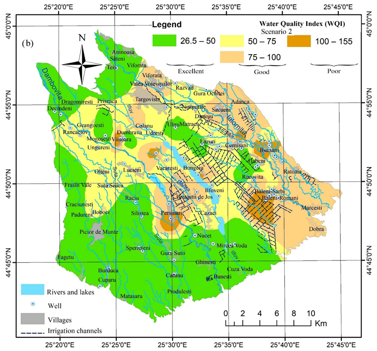
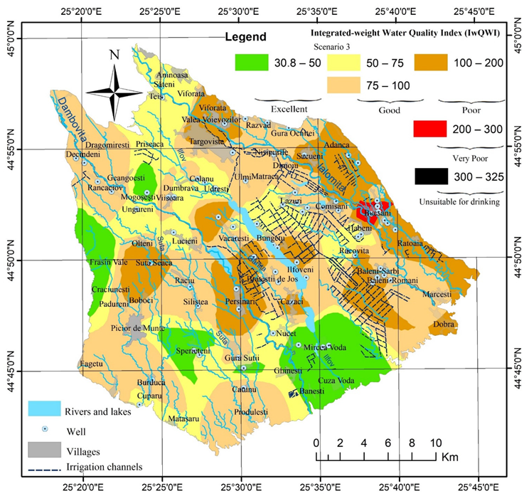
| Excellent (<50) | 39 | 48.75 | 27 | 33.75 | 8 | 10 |
| Good (50–100) | 38 | 47.5 | 40 | 50 | 52 | 65 |
| Poor (100–200) | 3 | 3.75 | 13 | 16.25 | 17 | 21.25 |
| Very poor water (200–300) | - | - | - | - | 2 | 2.5 |
| Water is unsuitable for consumption (>300) | - | - | - | - | 1 | 1.25 |
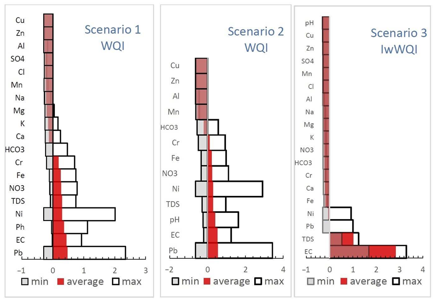
| Parameters | Scenario 1 Effective Weight (Ewi) (%) | Scenario 2 Effective Weight (Ewi) (%) | Scenario 3 Effective Weight (Ewi) (%) | |||||||||
|---|---|---|---|---|---|---|---|---|---|---|---|---|
| Min | Max | Average | STD | Min | Max | Average | STD | Min | Max | Average | STD | |
| Ca2+ [mg/L] | 0.91 | 9.66 | 3.01 | 1.51 | - | - | - | - | 0.31 | 4.60 | 1.49 | 0.80 |
| Mg2+ [mg/L] | 0.58 | 6.00 | 1.62 | 0.93 | - | - | - | - | 0.20 | 2.34 | 0.71 | 0.44 |
| Na+ [mg/L] | 0.38 | 4.13 | 1.29 | 0.67 | - | - | - | - | 0.14 | 2.04 | 0.67 | 0.36 |
| K+ [mg/L] | 0.76 | 8.37 | 2.58 | 1.35 | - | - | - | - | 0.17 | 2.52 | 0.82 | 0.45 |
| Cl− [mg/L] | 0.31 | 1.66 | 0.83 | 0.32 | - | - | - | - | 0.03 | 0.32 | 0.14 | 0.05 |
| SO42− [mg/L] | 0.34 | 1.76 | 0.81 | 0.32 | - | - | - | - | 0.02 | 0.20 | 0.07 | 0.03 |
| HCO3− [mg/L] | 1.06 | 13.64 | 4.93 | 2.41 | 1.09 | 14.50 | 5.22 | 2.67 | 0.29 | 3.99 | 1.25 | 0.67 |
| pH | 4.58 | 25.54 | 11.82 | 4.85 | 4.74 | 27.23 | 12.53 | 5.32 | 0.2 | 0.15 | 0.04 | 0.07 |
| EC [μS/cm] | 4.88 | 21.91 | 13.26 | 4.11 | 5.17 | 22.70 | 13.98 | 4.37 | 35.69 | 64.6 | 54.46 | 6.22 |
| TDS | 3.87 | 18.55 | 10.64 | 3.41 | 4.10 | 19.22 | 11.22 | 3.62 | 14.83 | 27.7 | 23.66 | 2.80 |
| Fe [mg/L] | 3.36 | 18.7 | 9.88 | 3.52 | 3.56 | 19.54 | 10.40 | 3.69 | 0.85 | 3.85 | 1.98 | 0.56 |
| Mn [mg/L] | 0.17 | 2.41 | 1.06 | 0.42 | 0.18 | 2.56 | 1.12 | 0.45 | 0.03 | 0.24 | 0.13 | 0.03 |
| NO3− [mg/L] | 3.55 | 19.50 | 10.09 | 3.38 | 3.64 | 20.97 | 10.58 | 3.72 | 0.24 | 2.54 | 1.10 | 0.39 |
| Cr [mg/L] | 1.69 | 17.96 | 8.63 | 4.41 | 1.77 | 18.86 | 9.00 | 4.62 | 0.40 | 2.38 | 1.31 | 0.49 |
| Pb2+ [mg/L] | 0.03 | 47.50 | 19.35 | 13.07 | 0.03 | 48.91 | 19.96 | 13.41 | 0.007 | 23.35 | 7.92 | 6.35 |
| Ni2+ [mg/L] | 0.07 | 41.7 | 14.97 | 6.99 | 0.07 | 42.59 | 15.67 | 7.30 | 0.01 | 21.83 | 5.99 | 3.46 |
| Zn [mg/L] | 0.02 | 0.45 | 0.16 | 0.11 | 0.02 | 0.46 | 0.16 | 0.10 | 0.005 | 0.24 | 0.07 | 0.05 |
| Al [mg/L] | 0.06 | 2.26 | 0.53 | 0.44 | 0.06 | 2.33 | 0.55 | 0.45 | 0.02 | 1.09 | 0.29 | 0.26 |
| Cu [mg/L] | 0.03 | 0.25 | 0.07 | 0.03 | 0.01 | 0.26 | 0.07 | 0 | 0.0002 | 0.05 | 0.01 | 0.01 |
| HQ Oral | HQ Dermal | |||||||
|---|---|---|---|---|---|---|---|---|
| Average | Max | Min | Stdev | Average | Max | Min | Stdev | |
| Mn | 4.93 × 10⁻⁵ | 2.02 × 10⁻⁴ | 1.19 × 10⁻⁵ | 2.90 × 10⁻⁵ | 6.16 × 10⁻⁶ | 2.53 × 10⁻⁵ | 1.49 × 10⁻⁶ | 3.63 × 10⁻⁶ |
| Ni | 4.80 × 10⁻² | 1.26 × 10⁻¹ | 1.42 × 10⁻⁴ | 2.50 × 10⁻² | 1.20 × 10⁻² | 3.14 × 10⁻² | 3.54 × 10⁻⁵ | 6.26 × 10⁻³ |
| Fe | 1.22 × 10⁻² | 4.98 × 10⁻² | 4.49 × 10⁻³ | 8.22 × 10⁻³ | 3.05 × 10⁻⁴ | 1.25 × 10⁻³ | 1.12 × 10⁻⁴ | 2.06 × 10⁻⁴ |
| NO3 | 6.47 × 10⁻¹ | 1.08 | 3.84 × 10⁻¹ | 1.53 × 10⁻¹ | 1.94 × 10⁻² | 3.24 × 10⁻² | 1.15 × 10⁻² | 4.60 × 10⁻³ |
| Cu | 9.01 × 10⁻³ | 2.50 × 10⁻² | 1.23 × 10⁻⁴ | 5.48 × 10⁻³ | 2.25 × 10⁻⁴ | 6.26 × 10⁻⁴ | 3.08 × 10⁻⁶ | 1.37 × 10⁻⁴ |
| Al | 1.30 × 10⁻³ | 5.11 × 10⁻³ | 8.49 × 10⁻⁵ | 1.19 × 10⁻³ | 3.25 × 10⁻⁵ | 1.28 × 10⁻⁴ | 2.13 × 10⁻⁶ | 2.98 × 10⁻⁵ |
| Zn | 4.27 × 10⁻³ | 1.23 × 10⁻² | 2.80 × 10⁻⁴ | 3.23 × 10⁻³ | 6.41 × 10⁻⁵ | 1.85 × 10⁻⁴ | 4.20 × 10⁻⁶ | 4.85 × 10⁻⁵ |
| Cr | 3.24 × 10⁻¹ | 8.57 × 10⁻¹ | 9.52 × 10⁻² | 1.90 × 10⁻¹ | 1.30 × 10⁻¹ | 3.43 × 10⁻¹ | 3.81 × 10⁻² | 7.62 × 10⁻² |
| Pb | 3.98 × 10⁻¹ | 1.23 | 3.32 × 10⁻⁴ | 3.29 × 10⁻¹ | 6.65 × 10⁻³ | 2.05 × 10⁻² | 5.53 × 10⁻⁶ | 5.49 × 10⁻³ |
| THI | HQ oral | HQ dermal | CCR | CCR | |||
|---|---|---|---|---|---|---|---|
| Ni | Cr | Pb | |||||
| average | 1.47 | 1.31 | 0.16 | 1.15 × 10⁻² | 8.17 × 10⁻³ | 4.67 × 10⁻⁵ | 7.97 × 10⁻³ |
| max | 2.97 | 2.64 | 0.33 | 3.92 × 10⁻² | 2.14 × 10⁻² | 1.25 × 10⁻⁴ | 2.46 × 10⁻² |
| min | 0.64 | 0.59 | 0.05 | 1.39 × 10⁻⁵ | 2.41 × 10⁻⁵ | 1.39 × 10⁻⁵ | 6.63 × 10⁻⁶ |
| stdev | 0.56 | 0.50 | 0.07 | 1.01 × 10⁻² | 4.26 × 10⁻³ | 2.80 × 10⁻⁵ | 6.58 × 10⁻³ |
Publisher’s Note: MDPI stays neutral with regard to jurisdictional claims in published maps and institutional affiliations. |
© 2022 by the authors. Licensee MDPI, Basel, Switzerland. This article is an open access article distributed under the terms and conditions of the Creative Commons Attribution (CC BY) license (https://creativecommons.org/licenses/by/4.0/).
Share and Cite
Bretcan, P.; Tanislav, D.; Radulescu, C.; Serban, G.; Danielescu, S.; Reid, M.; Dunea, D. Evaluation of Shallow Groundwater Quality at Regional Scales Using Adaptive Water Quality Indices. Int. J. Environ. Res. Public Health 2022, 19, 10637. https://doi.org/10.3390/ijerph191710637
Bretcan P, Tanislav D, Radulescu C, Serban G, Danielescu S, Reid M, Dunea D. Evaluation of Shallow Groundwater Quality at Regional Scales Using Adaptive Water Quality Indices. International Journal of Environmental Research and Public Health. 2022; 19(17):10637. https://doi.org/10.3390/ijerph191710637
Chicago/Turabian StyleBretcan, Petre, Danut Tanislav, Cristiana Radulescu, Gheorghe Serban, Serban Danielescu, Michael Reid, and Daniel Dunea. 2022. "Evaluation of Shallow Groundwater Quality at Regional Scales Using Adaptive Water Quality Indices" International Journal of Environmental Research and Public Health 19, no. 17: 10637. https://doi.org/10.3390/ijerph191710637