China’s Provincial Eco-Efficiency and Its Driving Factors—Based on Network DEA and PLS-SEM Method


Abstract
:1. Introduction
2. Research Method and Data
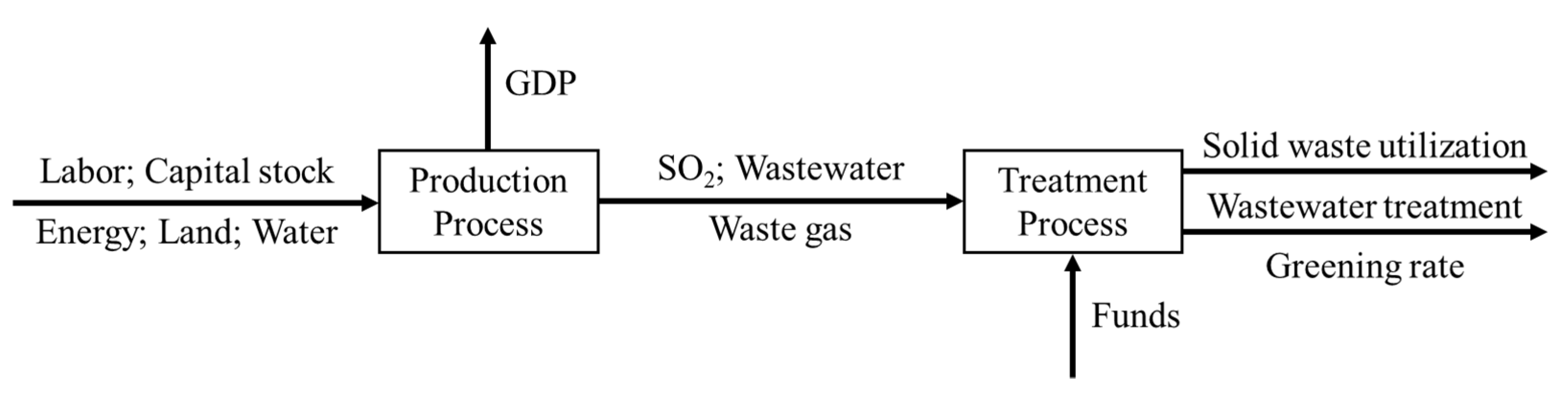
2.1. Two-Stage Network DEA
2.2. PLS-SEM Model
2.3. Data Sources
3. Result and Discussion
3.1. Analysis of Regional Eco-Efficiency of Different Provincial Administrative Regions in China
3.2. Eco-Efficiency Analysis of China’s Regional Production Process
3.3. Analysis of the Efficiency of China’s Provincial Environmental Treatment
4. Analysis of the Driving Factors of China’s Eco-Efficiency
4.1. Selection of Indexes
4.2. The Construction of the Estimation Model
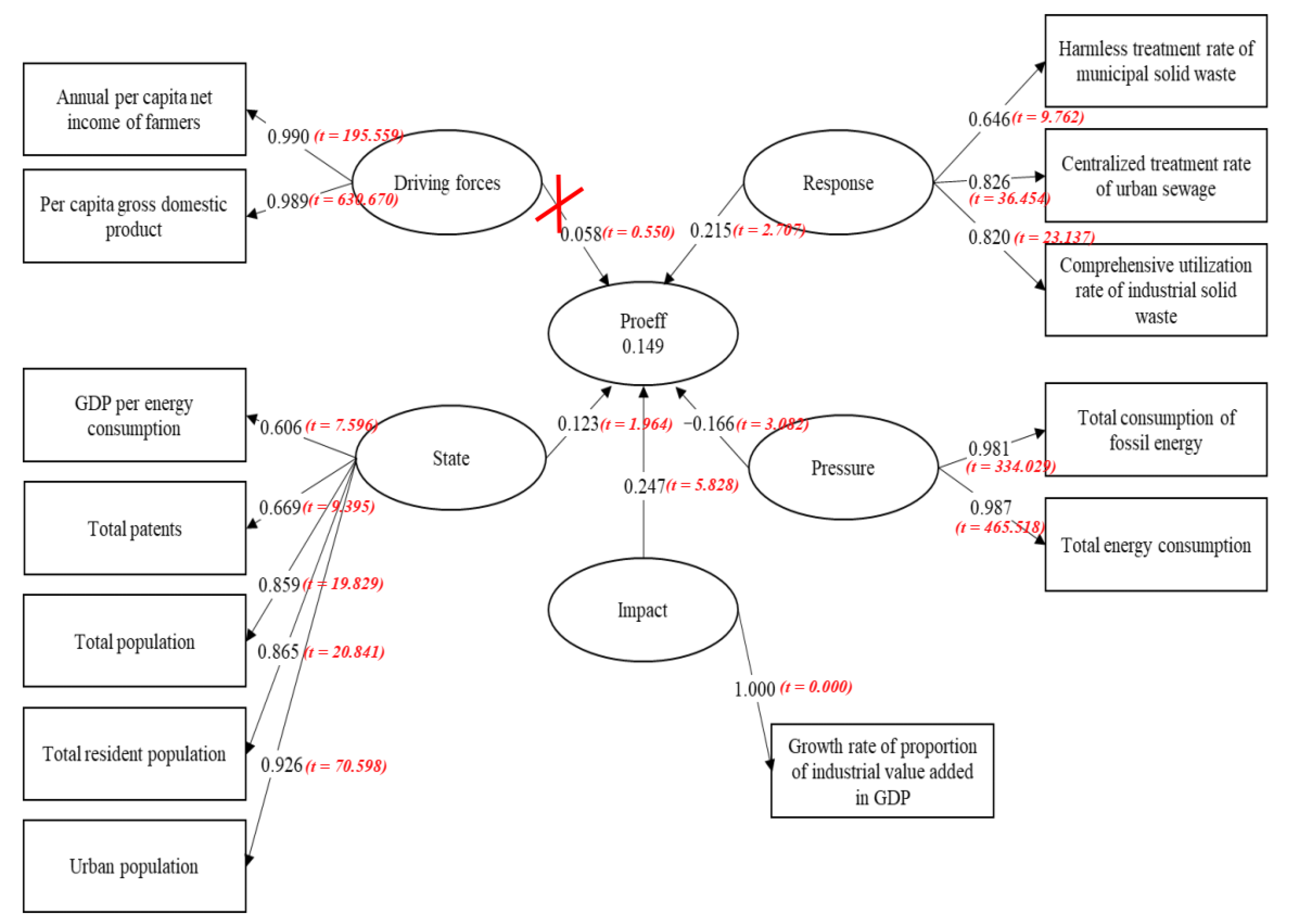
4.3. Analysis of the Driving Factors of the Production Stage
- (1)
- The influence coefficient between impact and production efficiency is 0.247, which indicates that the factor of impact has prominent positive influence on the environmental production efficiency. Its influence is the largest among the indexes, which is represented by the fact that a high proportion of industrial value added in the GDP entails increased environmental production efficiency. On the one hand, the expansion of the industrial value-added proportion of GDP demonstrates the enhanced capability of industrial production. On the other hand, it indicates progressing industrial technology innovation. Improvement in industrial technology innovation also decreases the overall energy consumption and pollution brought by industrial products. To some extent, it demonstrates the improvement of the environmental production efficiency.
- (2)
- The response system influences the production efficiency to a certain degree. The influence coefficient is 0.215, which means that a collective sewage treatment by an industrial solid waste treatment plant and its comprehensive utilization increases the production efficiency as the province puts more effort into the decontamination of urban refuse. Li and Liu [74] found that technological innovation is the principal force for promoting green and inclusive all-factor productivity. They believe that enhancing the production efficiency should be the key to numerous challenges, such as sustaining development, eradicating poverty, saving natural resources and protecting the environment.
- (3)
- The pathway coefficient of state and production efficiency is 0.123, thus reflecting a positive influence on the production efficiency exerted by the value of the state. However, this influence is the most trivial. The production efficiency would improve correspondingly with the increase of the per capita GDP’s consumption of energy due to the number of patents being passed, the urban population, the total number of permanent population and the total population. In fact, the population, which includes the urban population and the permanent population, is a factor closely related to the environment. The increase of these parameters leads to substantial labor force provision. In addition, the labor force could significantly enhance the production efficiency. The growing number of patents indicates higher innovative ability, which also improves the production efficiency.
- (4)
- Pressure is the only index that shows an evident negative influence on the production eco-efficiency. The pathway coefficient is −0.166, which indicates that enlarging the overall consumption of energy and fossil fuels brings about low production eco-efficiency. Therefore, a larger consumption of energy and fossil fuel lowers the energy-utilizing efficiency in China. Fossil fuels not only elicit tremendous pollution but also characterize China’s industrial structure, where the secondary industry remains the largest. This circumstance hinders the country’s adjustment of the industrial structure and the enhancement of the innovative ability. All these factors contribute to low production eco-efficiency.
4.4. Analysis of the Driving Factors of the Treatment Stage
- (1)
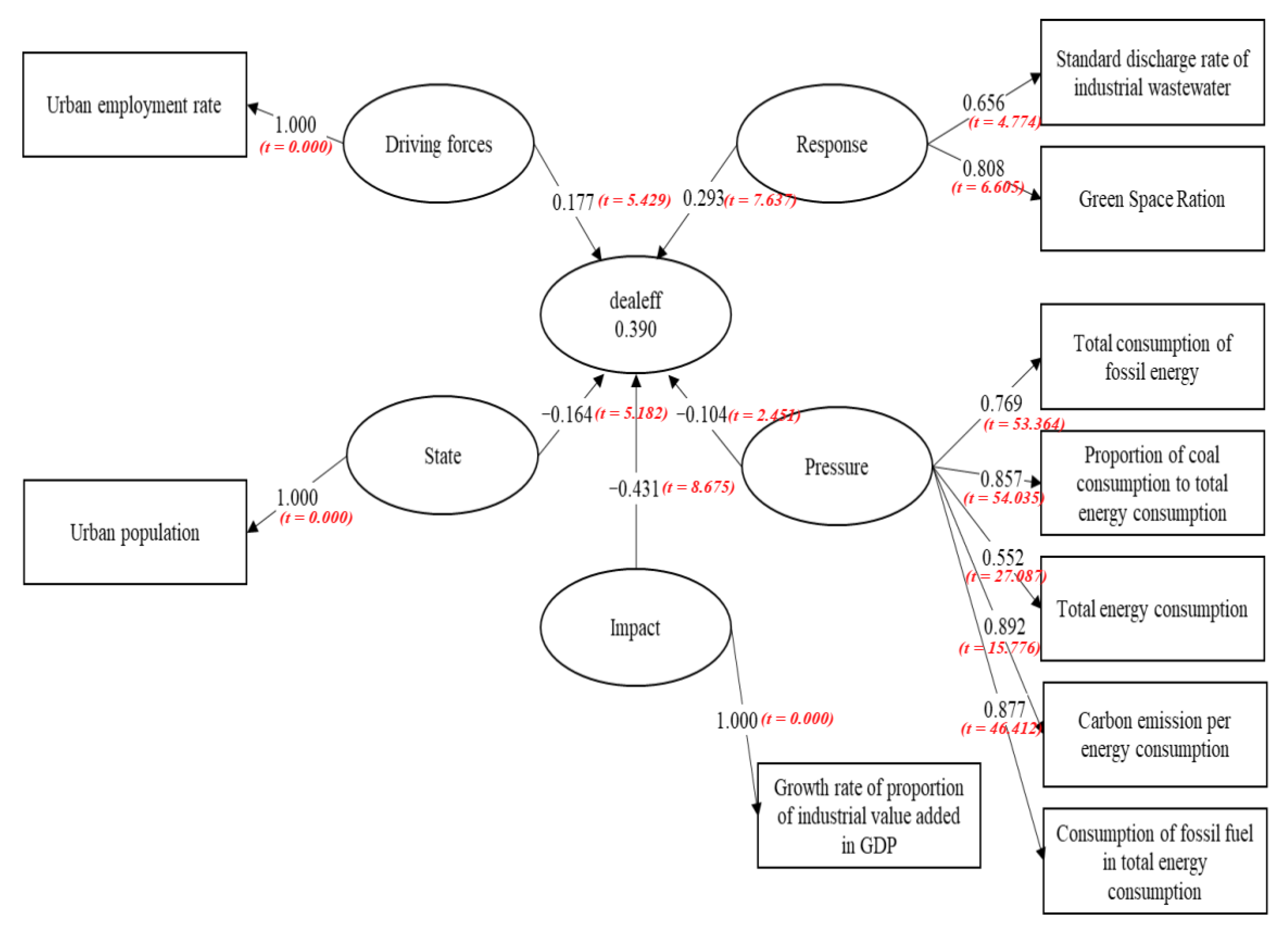
- The pathway coefficient of the driving factors and the environmental treatment efficiency is 0.177. This value shows that a higher urban employment rate increases the environmental treatment efficiency correspondingly. Thus, the population and the environment are always closely connected. When urbanization continues to expand, the labor force also increases. As a result, the urban employment rate and the city’s development rise. This cycle is beneficial to the city. With the increase in the employment rate and the development of the city, the labor force in the area where environmental management is implemented also steadily increases along with the improved population quality and efficiency in environmental treatment. Therefore, regions with poor human resources bases need to increase investment in human resources development and introduce and cultivate high-tech talents, in order to promote the development of high-tech industries [48].
- (2)
- The response system exerts a relatively large impact on the environmental treatment efficiency, which is represented by an influence coefficient of 0.293. This value indicates a higher afforestation rate. In addition, the control rate of industrial sewage discharge stimulates the environmental management rate. Afforestation is one of the crucial methods of environmental management. Generally, the high afforestation rate of a city entails better environmental treatment efficiency. Currently, water pollution is one major difficulty faced by urban environmental treatment, as the pollution caused by industrial wastewater is rather severe. Thus, when the control rate of industrial sewage discharge is higher, the city’s environmental treatment efficiency also increases.
- (3)
- The influence coefficient of the influencing factors and the environmental treatment efficiency is −0.431, which mainly reflects an inversion between the expanding industrial proportion in the GDP value added and the environmental treatment efficiency. The most important index is the industrial proportion in the GDP value added, which signifies that industrial pollution exerts a considerable impact on the environmental treatment efficiency. Given that the ratio of the secondary industry in China is still high, the improvement of the environmental treatment efficiency is hindered, which indicates that the industrial structure of our country needs to be adjusted.
- (4)
- Moreover, the pressure system has an evident negative impact on environmental treatment efficiency. The pathway coefficient between the two factors is −0.104, as shown by the result of the model. Carbon emission and energy consumption is an important indicator of environmental treatment efficiency. The major contributors are the consumption of fossil fuel. The high ratio of fossil fuel and coal consumption lowers the environmental treatment efficiency. The overall energy consumption, particularly the overall consumption of fossil fuel itself, greatly pollutes the environment, which is at odds with environmental treatment. Thus, a greater overall energy consumption and fossil fuel consumption increases the severity of the pollution. Moreover, the increase in consumption decreases the environmental treatment efficiency.
- (5)
- The pathway coefficient of the state and the environmental treatment efficiency is −0.164, which means that state indeed influences environmental treatment efficiency negatively. With an increasingly urban population, environmental treatment efficiency decreases. China is still a developing country at its current stage. The concept of energy conservation and environmental protection is insufficient, which will lead to the decline of ecological efficiency [75]. From the perspective of the pathway coefficient, the influence remains comparatively low even though the index of the urban population evidently negatively affects the environmental treatment efficiency.
4.5. Analysis of the Driving Factors of Overall Efficiency
5. Conclusions
- (1)
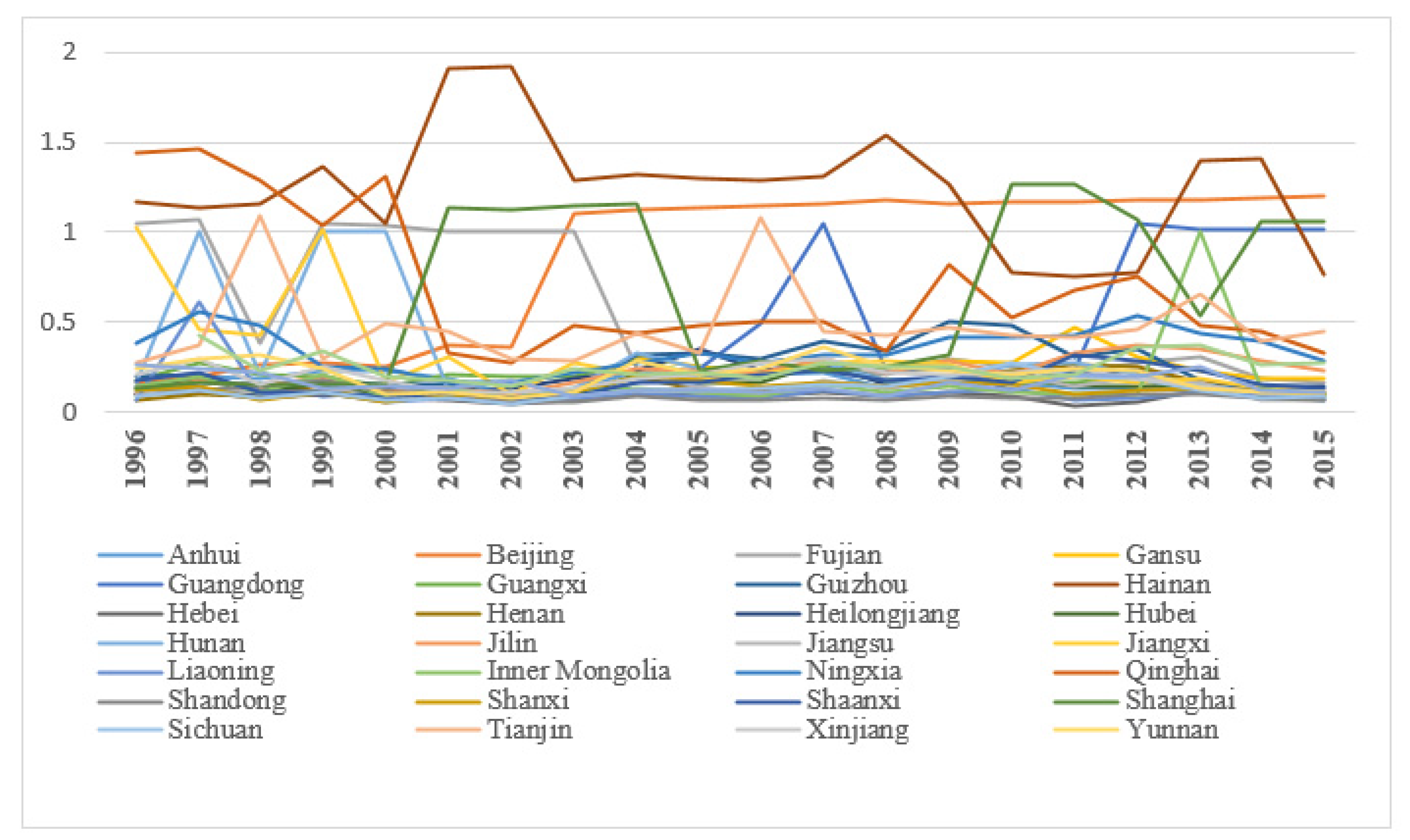
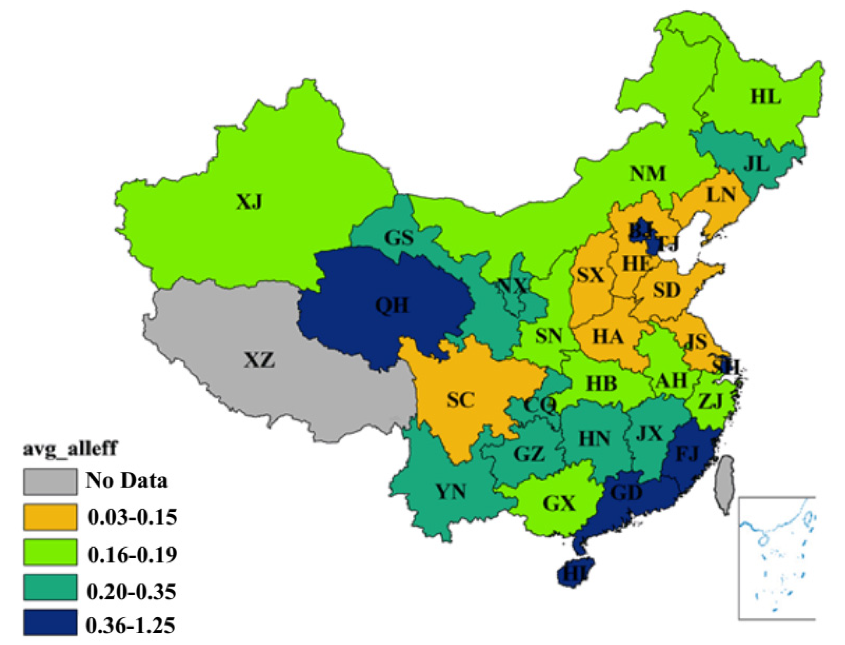
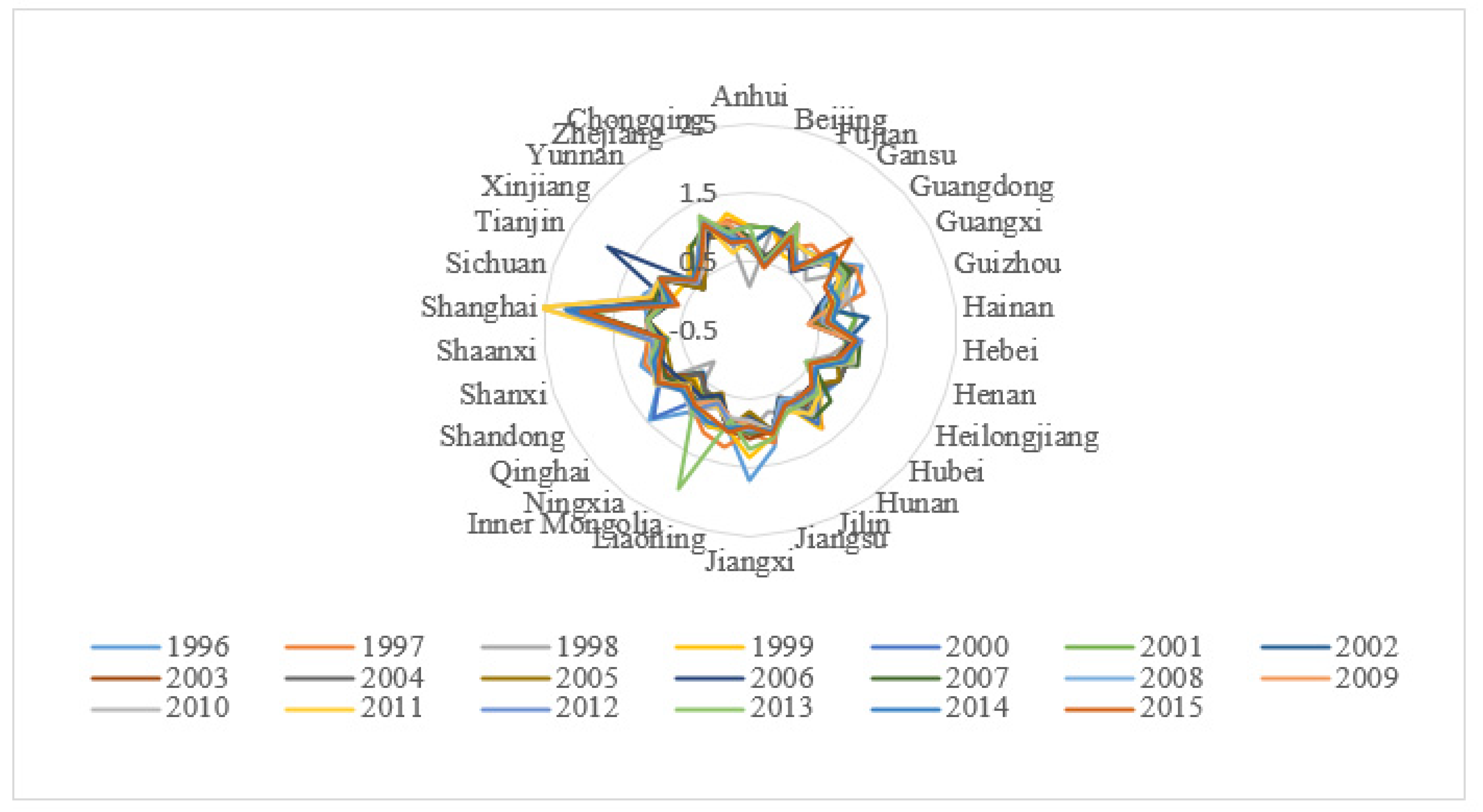
- The overall eco-efficiency of various provincial administrative regions manifests greatly different trends from 1996 to 2015. In most regions, the eco-efficiency was below 1, indicating that they were less efficient. From a spatial perspective, eco-efficiency varied greatly between 30 provincial administrative regions due to different levels of economic development and environmental protection. The average eco-efficiencies of 30 different regions in China fell into four sections: 0.03–0.15, 0.16–0.19, 0.20–0.35 and 0.36–1.25. The average eco-efficiencies of Hainan, Guangdong, Fujian, Beijing, Tianjin, Qinghai and Shanghai were between 0.36 and 1.25, which are considerably high. Meanwhile, the eco-efficiencies of Hebei, Shandong and Henan were in the lowest group. In addition, the trend from the western areas to the southeast coastal areas gradually increased. From a chronological perspective, the production of most regions in China was comparatively low, without much fluctuation.
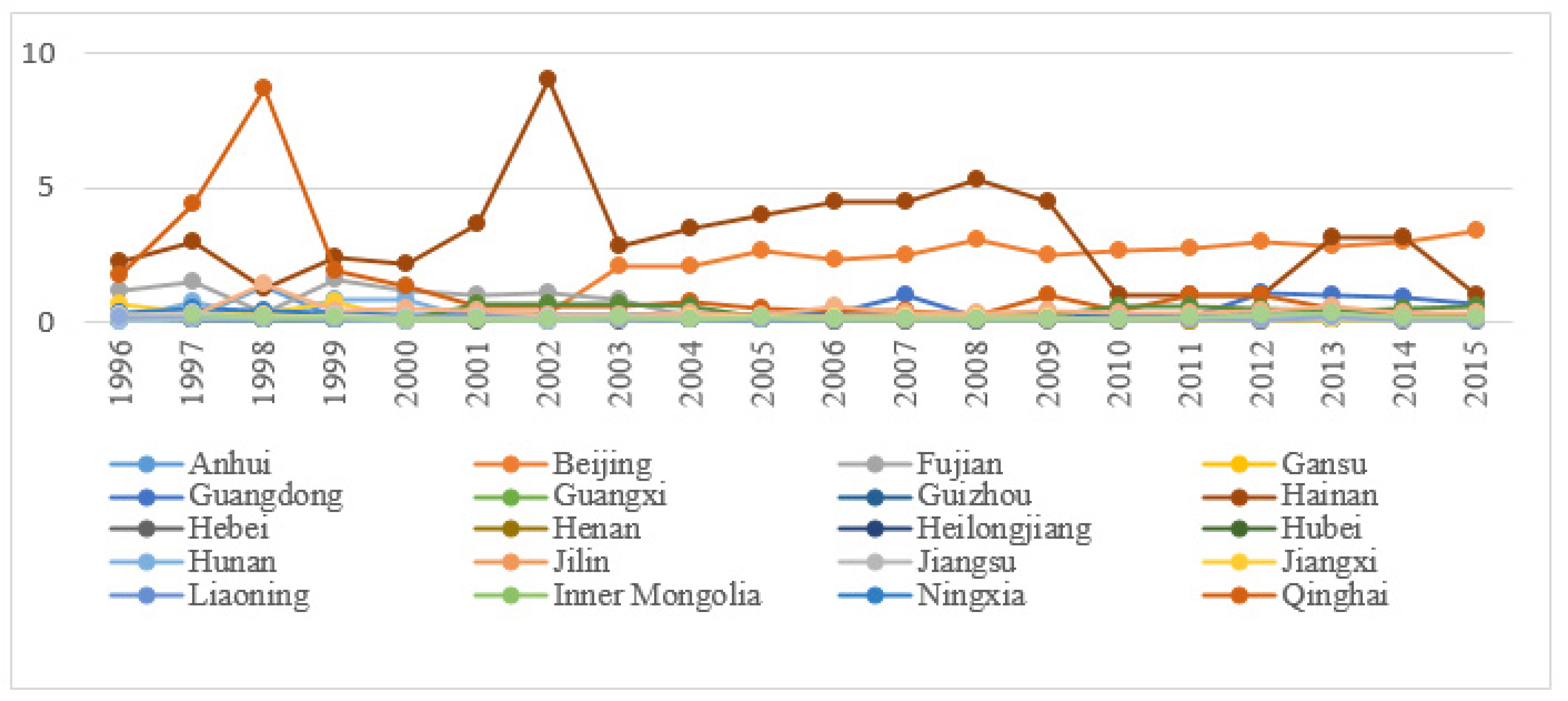
- (2)
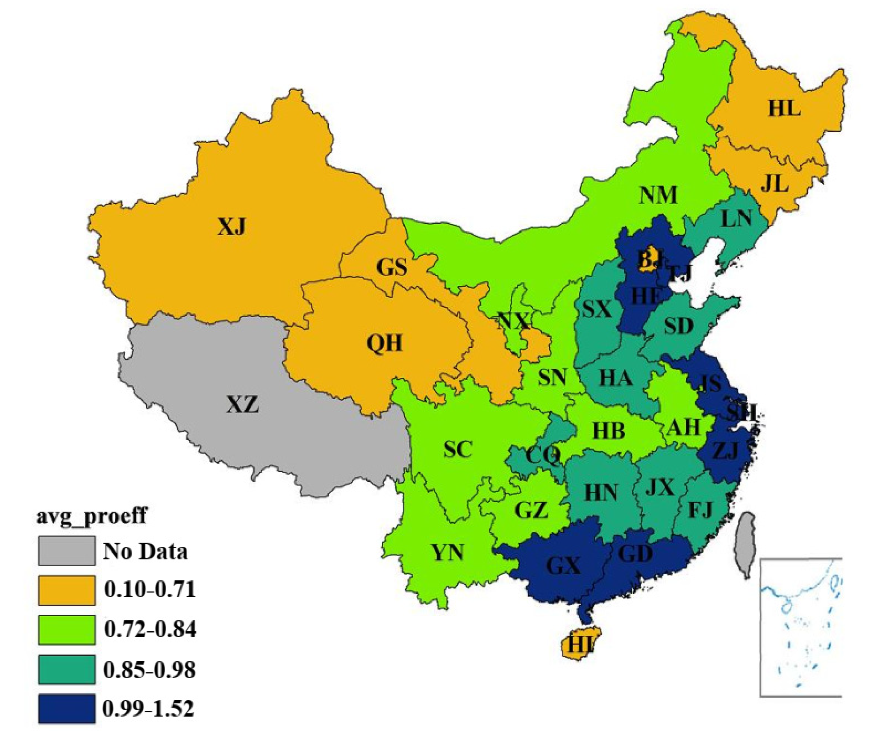
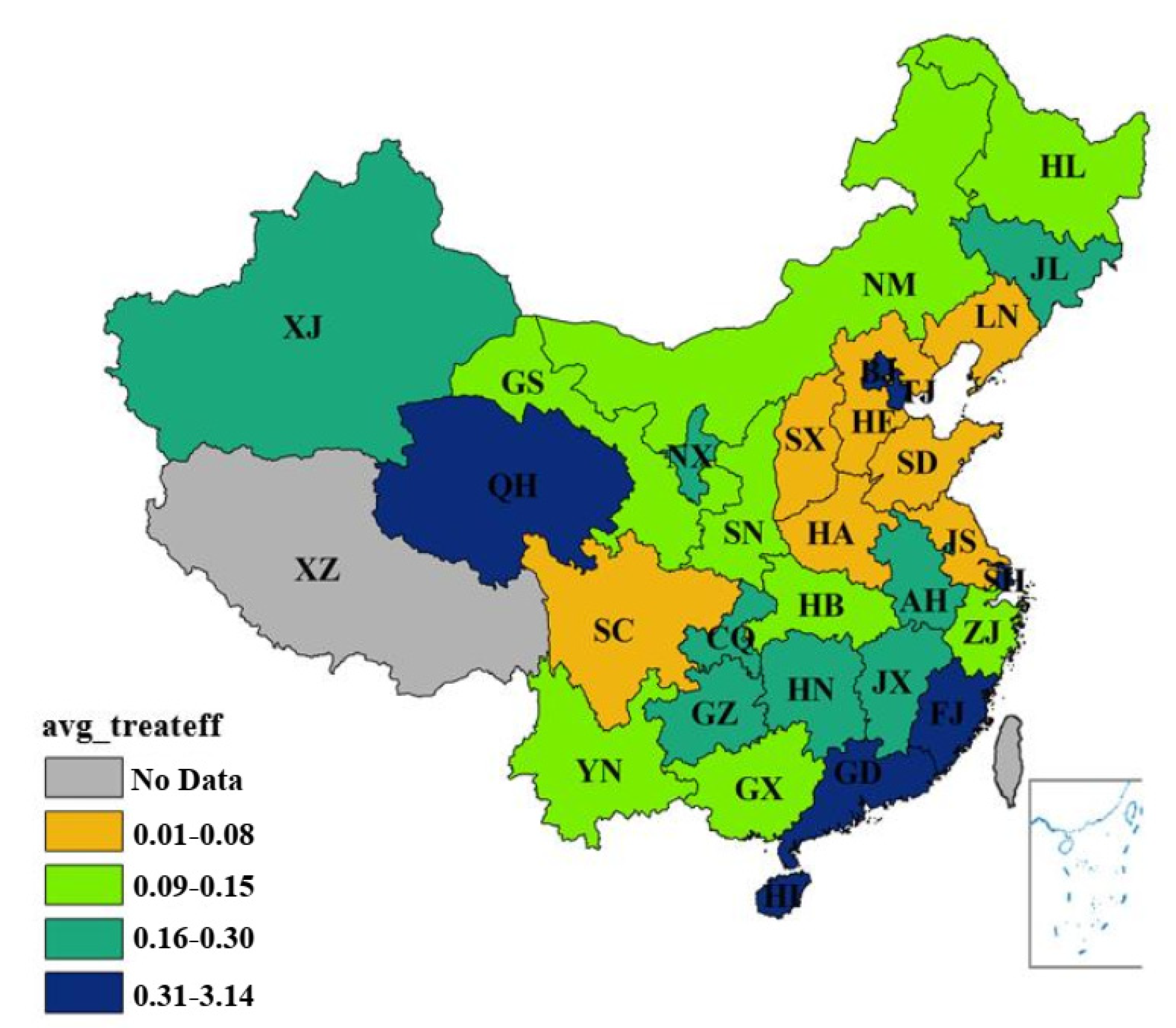
- The two-stage DEA model divides the eco-efficiency into production efficiency and treatment efficiency. From a chronological perspective, different regions in China display diverse changes in various periods between 1996 and 2015. In general, the environmental production efficiency of most regions in China was comparatively low. The environmental treatment efficiency was also low, and the amplitudes were minor. From a spatial perspective, the average production efficiency of 30 regions (municipalities) in China fell into four sections: 0.10–0.71, 0.72–0.84, 0.85–0.98 and 0.99–1.52. An apparent trend of gradual increase was also observed from the western areas to the southeast coastal areas. Moreover, the environmental treatment efficiency of 30 provincial administrative regions in China increased from the north to the south.
- (3)
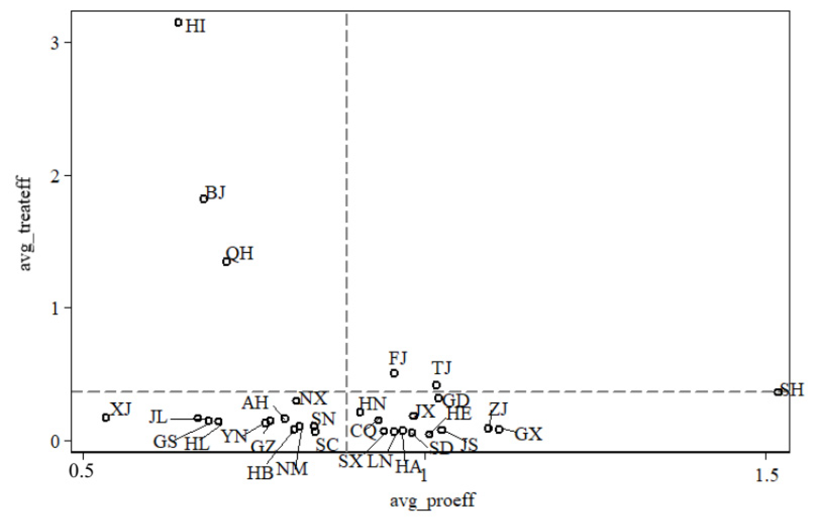
- When comparing the production efficiency with the environmental treatment efficiency, some important findings can be derived. Beijing, Qinghai and Hainan efficiency and the environmental treatment of Fujian and Tianjin were higher than the average. These regions show low levels of production efficiency and high levels of environmental treatment efficiency. The production efficiency and environmental treatment were low in the group of provincial administrative regions where economies were lagging behind the national average. For economically well-developed regions, the efficiency of the production stage evidently outweighed the average efficiency. Meanwhile, that of the environmental treatment stage was prominently lower than the average value.
- (4)
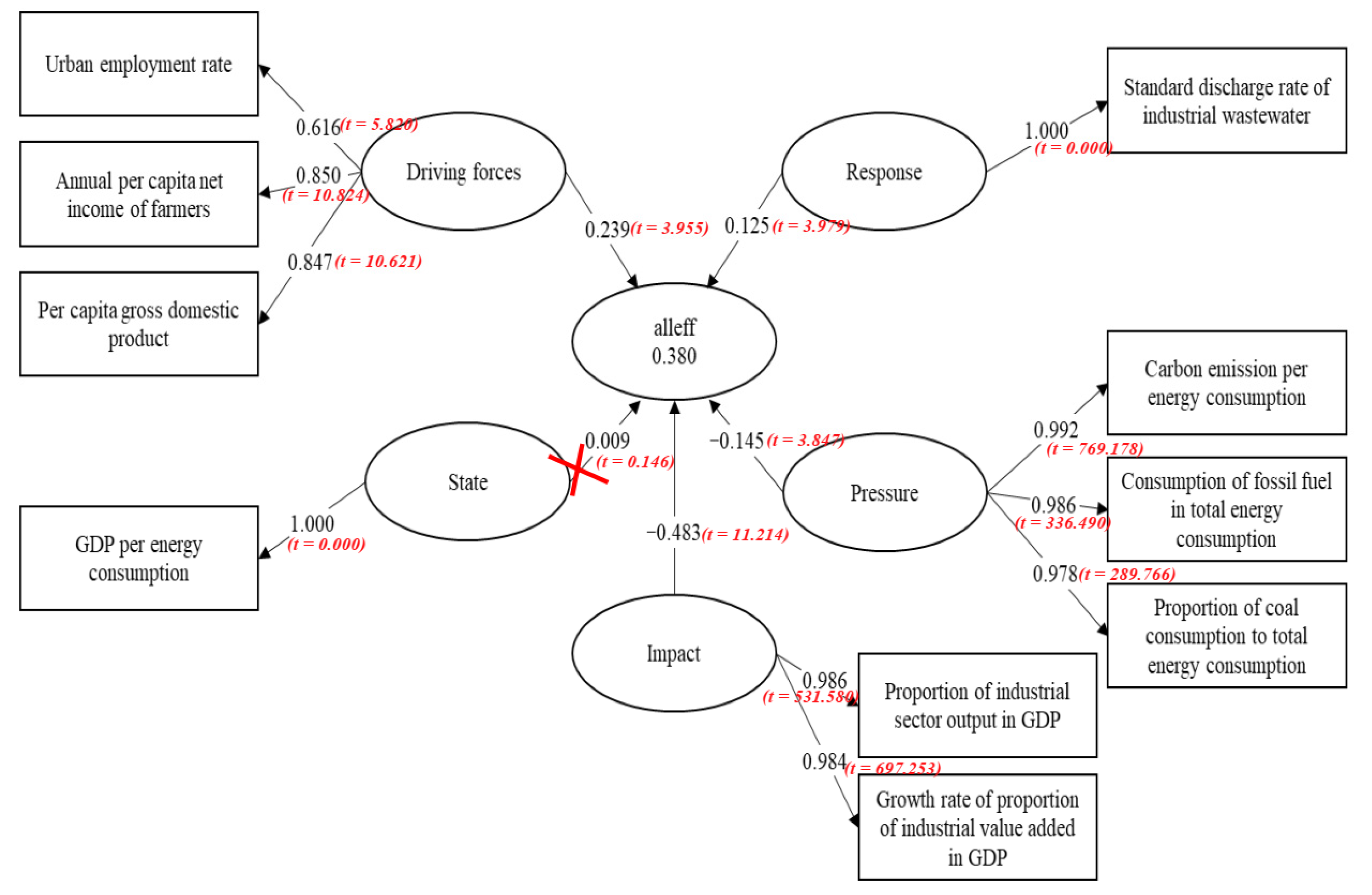
- Impact, response, state and pressure have remarkable influences on the eco-efficiency of the production stage, where the value of impact is the most influential among the indexes. Aside from the pressure system, other indexes all exerted positive influences on production efficiency. The driving forces, response, impact, pressure and state all significantly influenced the eco-efficiency of the management stage, where the response index was more influential. Except for driving forces and impact, other indexes negatively affected eco-efficiency. In terms of the overall eco-efficiency, the driving forces, response, impact and pressure were all important influencing factors, where impact exerted the most influence. The relationship between the driving forces and the overall eco-efficiency was positive, and the same was true with the response. Meanwhile, the influences of impact and pressure were negative.
Author Contributions
Funding
Conflicts of Interest
Appendix A

| Provinces | 1996 | 1997 | 1998 | 1999 | 2000 | 2001 | 2002 | 2003 | 2004 | 2005 | 2006 | 2007 | 2008 | 2009 | 2010 | 2011 | 2012 | 2013 | 2014 | 2015 |
|---|---|---|---|---|---|---|---|---|---|---|---|---|---|---|---|---|---|---|---|---|
| Anhui | 0.75 | 1.00 | 0.13 | 1.00 | 1.00 | 1.00 | 0.74 | 0.76 | 0.78 | 0.68 | 0.75 | 0.84 | 0.71 | 0.75 | 0.78 | 0.82 | 0.82 | 1.01 | 0.80 | 0.79 |
| Beijing | 1.00 | 1.00 | 1.00 | 1.00 | 1.00 | 1.00 | 1.00 | 0.58 | 0.61 | 0.49 | 0.56 | 0.53 | 0.44 | 0.53 | 0.50 | 0.49 | 0.46 | 0.48 | 0.46 | 0.41 |
| Fujian | 0.93 | 0.78 | 1.00 | 0.70 | 0.90 | 0.98 | 0.97 | 1.19 | 0.89 | 0.90 | 0.88 | 1.01 | 0.89 | 0.96 | 1.10 | 0.97 | 0.95 | 1.18 | 0.96 | 0.98 |
| Gansu | 0.91 | 1.04 | 0.87 | 0.68 | 0.64 | 0.62 | 0.57 | 0.63 | 0.64 | 0.59 | 0.54 | 0.61 | 0.67 | 0.66 | 0.60 | 0.91 | 0.69 | 0.60 | 0.63 | 0.57 |
| Guangdong | 1.00 | 1.00 | 0.58 | 0.92 | 1.00 | 1.00 | 1.00 | 1.00 | 1.00 | 1.00 | 1.00 | 1.14 | 1.00 | 1.00 | 1.00 | 1.00 | 1.04 | 1.08 | 1.16 | 1.50 |
| Guangxi | 1.37 | 1.29 | 1.16 | 1.19 | 1.16 | 1.26 | 1.22 | 1.19 | 1.24 | 1.06 | 1.05 | 1.17 | 1.03 | 1.03 | 1.01 | 1.01 | 1.09 | 1.10 | 0.82 | 0.75 |
| Guizhou | 1.07 | 1.24 | 1.00 | 0.90 | 0.69 | 0.66 | 0.58 | 0.53 | 0.55 | 0.56 | 0.54 | 0.71 | 0.60 | 0.87 | 0.99 | 0.73 | 0.80 | 0.80 | 0.88 | 0.76 |
| Hainan | 0.62 | 0.44 | 1.06 | 0.72 | 0.50 | 1.05 | 1.23 | 0.64 | 0.55 | 0.45 | 0.38 | 0.39 | 0.57 | 0.36 | 0.62 | 0.59 | 0.58 | 0.73 | 0.71 | 0.63 |
| Hebei | 0.98 | 1.00 | 1.00 | 0.88 | 0.92 | 0.89 | 0.93 | 1.00 | 1.09 | 0.99 | 1.00 | 1.11 | 1.00 | 1.01 | 1.01 | 1.06 | 1.14 | 1.01 | 1.07 | 1.06 |
| Henan | 1.00 | 1.00 | 0.75 | 1.00 | 1.00 | 1.00 | 1.00 | 1.00 | 0.99 | 0.84 | 0.86 | 1.16 | 0.97 | 0.93 | 1.09 | 1.05 | 0.89 | 1.04 | 0.97 | 0.85 |
| Heilongjiang | 1.00 | 1.00 | 0.44 | 0.61 | 1.00 | 0.50 | 1.00 | 1.00 | 1.00 | 1.00 | 0.52 | 0.58 | 0.52 | 0.49 | 0.58 | 0.58 | 0.59 | 0.45 | 0.62 | 0.51 |
| Hubei | 0.91 | 0.77 | 0.89 | 0.89 | 0.86 | 0.74 | 0.72 | 0.77 | 0.81 | 0.70 | 0.71 | 1.06 | 0.75 | 0.73 | 0.85 | 0.88 | 0.81 | 0.86 | 0.76 | 0.73 |
| Hunan | 0.87 | 1.28 | 0.65 | 1.26 | 1.18 | 0.90 | 0.90 | 0.86 | 0.99 | 0.76 | 0.71 | 1.09 | 0.73 | 0.75 | 1.05 | 1.00 | 0.84 | 0.83 | 0.73 | 0.73 |
| Jilin | 0.63 | 0.63 | 0.84 | 0.67 | 0.62 | 0.60 | 0.56 | 0.59 | 0.61 | 0.61 | 0.60 | 0.68 | 0.62 | 0.72 | 0.66 | 0.81 | 0.67 | 0.80 | 0.72 | 0.72 |
| Jiangsu | 1.24 | 1.17 | 0.72 | 1.09 | 1.00 | 1.03 | 1.03 | 1.00 | 1.00 | 1.00 | 1.00 | 1.00 | 1.00 | 1.00 | 1.00 | 1.00 | 1.00 | 1.12 | 1.04 | 1.05 |
| Jiangxi | 1.68 | 1.00 | 1.00 | 1.36 | 1.00 | 1.00 | 0.74 | 1.08 | 0.80 | 0.70 | 0.79 | 1.00 | 0.97 | 0.87 | 0.82 | 0.91 | 0.94 | 1.24 | 0.89 | 0.90 |
| Liaoning | 1.00 | 1.24 | 1.00 | 1.00 | 1.00 | 1.00 | 1.00 | 1.00 | 0.90 | 0.96 | 0.90 | 0.90 | 0.93 | 0.82 | 0.80 | 0.91 | 0.89 | 0.85 | 0.98 | 1.04 |
| Inner Mongolia | 1.04 | 1.14 | 0.90 | 1.03 | 0.68 | 0.67 | 0.67 | 0.64 | 0.60 | 0.51 | 0.54 | 0.61 | 0.64 | 0.65 | 0.75 | 0.69 | 0.67 | 2.04 | 0.98 | 0.90 |
| Ningxia | 0.98 | 0.93 | 1.00 | 0.72 | 0.76 | 0.65 | 0.61 | 0.60 | 0.61 | 0.71 | 0.72 | 0.82 | 0.83 | 0.84 | 0.97 | 0.89 | 0.93 | 0.90 | 0.92 | 0.86 |
| Qinghai | 1.47 | 0.62 | 0.20 | 0.55 | 1.40 | 0.43 | 0.41 | 0.46 | 0.47 | 0.61 | 0.69 | 0.73 | 0.76 | 0.82 | 0.82 | 0.70 | 0.76 | 0.75 | 0.81 | 0.73 |
| Shandong | 1.00 | 1.00 | 1.00 | 1.00 | 1.00 | 1.00 | 0.95 | 0.88 | 0.98 | 0.82 | 0.79 | 0.91 | 0.99 | 0.98 | 1.07 | 1.09 | 1.07 | 1.02 | 1.05 | 1.05 |
| Shanxi | 1.17 | 1.11 | 1.00 | 0.93 | 0.84 | 0.85 | 0.84 | 0.90 | 0.96 | 0.75 | 0.88 | 0.92 | 1.04 | 0.90 | 1.01 | 0.93 | 0.95 | 1.00 | 0.96 | 0.87 |
| Shaanxi | 0.99 | 1.01 | 0.95 | 0.71 | 0.78 | 0.70 | 0.72 | 0.77 | 0.84 | 0.75 | 0.76 | 0.84 | 0.90 | 0.87 | 0.89 | 0.96 | 0.93 | 0.86 | 0.77 | 0.77 |
| Shanghai | 1.00 | 1.00 | 1.00 | 1.00 | 1.00 | 1.84 | 1.94 | 1.93 | 2.18 | 1.00 | 1.00 | 1.00 | 1.00 | 1.00 | 2.58 | 2.58 | 2.16 | 1.00 | 2.19 | 1.97 |
| Sichuan | 1.14 | 0.90 | 0.91 | 0.75 | 0.87 | 0.80 | 0.81 | 0.99 | 0.79 | 0.71 | 0.73 | 0.96 | 0.78 | 0.82 | 1.08 | 1.00 | 0.66 | 0.77 | 0.71 | 0.61 |
| Tianjin | 0.92 | 1.02 | 0.87 | 0.67 | 1.00 | 1.00 | 1.00 | 1.00 | 1.00 | 1.00 | 1.89 | 1.00 | 1.00 | 1.00 | 1.00 | 1.00 | 1.00 | 1.00 | 1.00 | 1.00 |
| Xinjiang | 0.68 | 0.64 | 0.59 | 0.68 | 0.41 | 0.40 | 0.41 | 0.40 | 0.44 | 0.41 | 0.52 | 0.59 | 0.52 | 0.51 | 0.54 | 0.58 | 0.54 | 0.63 | 0.63 | 0.56 |
| Yunnan | 1.00 | 1.00 | 1.00 | 1.00 | 0.68 | 0.63 | 0.62 | 0.69 | 0.81 | 0.59 | 0.64 | 0.98 | 0.67 | 0.62 | 0.62 | 0.81 | 0.79 | 0.69 | 0.78 | 0.72 |
| Zhejiang | 1.00 | 1.00 | 1.00 | 1.00 | 1.00 | 1.00 | 1.00 | 1.00 | 1.00 | 1.04 | 1.03 | 1.13 | 1.18 | 1.18 | 1.18 | 1.26 | 1.24 | 1.32 | 1.15 | 1.18 |
| Chongqing | 1.14 | 0.87 | 1.21 | 0.98 | 0.93 | 0.89 | 0.90 | 1.04 | 0.85 | 1.04 | 1.05 | 0.93 | 1.06 | 0.85 | 0.65 | 0.77 | 0.94 | 0.84 | 0.79 |
| Provinces | 1996 | 1997 | 1998 | 1999 | 2000 | 2001 | 2002 | 2003 | 2004 | 2005 | 2006 | 2007 | 2008 | 2009 | 2010 | 2011 | 2012 | 2013 | 2014 | 2015 |
|---|---|---|---|---|---|---|---|---|---|---|---|---|---|---|---|---|---|---|---|---|
| Anhui | 0.13 | 0.15 | 1.30 | 0.15 | 0.14 | 0.12 | 0.09 | 0.09 | 0.13 | 0.13 | 0.11 | 0.11 | 0.09 | 0.10 | 0.08 | 0.06 | 0.07 | 0.07 | 0.06 | 0.05 |
| Beijing | 0.14 | 0.15 | 0.23 | 0.25 | 0.18 | 0.34 | 0.36 | 2.10 | 2.06 | 2.62 | 2.31 | 2.48 | 3.07 | 2.50 | 2.69 | 2.70 | 2.95 | 2.82 | 3.00 | 3.38 |
| Fujian | 1.19 | 1.45 | 0.35 | 1.59 | 1.19 | 1.03 | 1.04 | 0.84 | 0.14 | 0.12 | 0.11 | 0.11 | 0.11 | 0.14 | 0.11 | 0.10 | 0.14 | 0.19 | 0.11 | 0.09 |
| Gansu | 0.07 | 0.08 | 0.08 | 0.11 | 0.08 | 0.11 | 0.08 | 0.10 | 0.18 | 0.18 | 0.15 | 0.16 | 0.15 | 0.18 | 0.17 | 0.33 | 0.18 | 0.22 | 0.16 | 0.15 |
| Guangdong | 0.06 | 0.11 | 0.20 | 0.06 | 0.07 | 0.07 | 0.06 | 0.06 | 0.09 | 0.15 | 0.36 | 0.97 | 0.13 | 0.14 | 0.09 | 0.13 | 1.06 | 0.96 | 0.88 | 0.69 |
| Guangxi | 0.07 | 0.13 | 0.12 | 0.10 | 0.07 | 0.09 | 0.09 | 0.08 | 0.11 | 0.09 | 0.09 | 0.09 | 0.07 | 0.08 | 0.07 | 0.06 | 0.07 | 0.08 | 0.07 | 0.06 |
| Guizhou | 0.11 | 0.11 | 0.07 | 0.10 | 0.10 | 0.12 | 0.09 | 0.11 | 0.19 | 0.23 | 0.18 | 0.20 | 0.21 | 0.30 | 0.29 | 0.14 | 0.21 | 0.10 | 0.06 | 0.06 |
| Hainan | 2.22 | 2.95 | 1.27 | 2.39 | 2.19 | 3.64 | 9.02 | 2.81 | 3.45 | 3.96 | 4.46 | 4.45 | 5.28 | 4.49 | 1.00 | 1.00 | 1.00 | 3.13 | 3.18 | 1.00 |
| Hebei | 0.05 | 0.07 | 0.05 | 0.06 | 0.04 | 0.04 | 0.03 | 0.04 | 0.04 | 0.05 | 0.04 | 0.04 | 0.04 | 0.05 | 0.04 | 0.02 | 0.02 | 0.06 | 0.06 | 0.05 |
| Henan | 0.05 | 0.07 | 0.09 | 0.09 | 0.07 | 0.07 | 0.05 | 0.06 | 0.09 | 0.06 | 0.06 | 0.06 | 0.06 | 0.09 | 0.09 | 0.11 | 0.13 | 0.08 | 0.06 | 0.05 |
| Heilongjiang | 0.07 | 0.08 | 0.19 | 0.19 | 0.10 | 0.14 | 0.11 | 0.13 | 0.14 | 0.23 | 0.21 | 0.19 | 0.12 | 0.15 | 0.11 | 0.12 | 0.14 | 0.18 | 0.12 | 0.12 |
| Hubei | 0.08 | 0.12 | 0.09 | 0.08 | 0.07 | 0.07 | 0.06 | 0.06 | 0.10 | 0.10 | 0.09 | 0.11 | 0.10 | 0.10 | 0.10 | 0.06 | 0.07 | 0.10 | 0.07 | 0.06 |
| Hunan | 0.11 | 0.78 | 0.19 | 0.79 | 0.85 | 0.09 | 0.06 | 0.08 | 0.15 | 0.13 | 0.11 | 0.11 | 0.10 | 0.09 | 0.11 | 0.12 | 0.11 | 0.10 | 0.07 | 0.05 |
| Jilin | 0.12 | 0.16 | 0.11 | 0.20 | 0.12 | 0.15 | 0.12 | 0.15 | 0.17 | 0.17 | 0.15 | 0.18 | 0.15 | 0.17 | 0.12 | 0.18 | 0.29 | 0.25 | 0.19 | 0.14 |
| Jiangsu | 0.05 | 0.08 | 0.14 | 0.06 | 0.09 | 0.05 | 0.04 | 0.05 | 0.06 | 0.09 | 0.05 | 0.11 | 0.08 | 0.10 | 0.12 | 0.07 | 0.11 | 0.09 | 0.04 | 0.04 |
| Jiangxi | 0.63 | 0.30 | 0.31 | 0.77 | 0.10 | 0.20 | 0.07 | 0.12 | 0.11 | 0.12 | 0.11 | 0.12 | 0.12 | 0.12 | 0.09 | 0.09 | 0.08 | 0.09 | 0.08 | 0.06 |
| Liaoning | 0.04 | 0.32 | 0.07 | 0.06 | 0.04 | 0.05 | 0.05 | 0.06 | 0.06 | 0.05 | 0.04 | 0.05 | 0.04 | 0.06 | 0.06 | 0.03 | 0.04 | 0.07 | 0.05 | 0.04 |
| Inner Mongolia | 0.09 | 0.10 | 0.09 | 0.11 | 0.07 | 0.12 | 0.07 | 0.08 | 0.09 | 0.09 | 0.07 | 0.09 | 0.07 | 0.09 | 0.06 | 0.07 | 0.06 | 0.49 | 0.08 | 0.06 |
| Ningxia | 0.34 | 0.47 | 0.39 | 0.31 | 0.21 | 0.22 | 0.23 | 0.23 | 0.29 | 0.29 | 0.23 | 0.24 | 0.25 | 0.34 | 0.25 | 0.29 | 0.40 | 0.39 | 0.33 | 0.22 |
| Qinghai | 1.76 | 4.41 | 8.68 | 1.93 | 1.35 | 0.58 | 0.56 | 0.62 | 0.74 | 0.49 | 0.45 | 0.40 | 0.29 | 1.00 | 0.46 | 1.00 | 1.00 | 0.50 | 0.37 | 0.28 |
| Shandong | 0.10 | 0.09 | 0.11 | 0.12 | 0.07 | 0.08 | 0.04 | 0.05 | 0.05 | 0.05 | 0.04 | 0.04 | 0.04 | 0.04 | 0.04 | 0.03 | 0.04 | 0.06 | 0.04 | 0.04 |
| Shanxi | 0.07 | 0.08 | 0.05 | 0.06 | 0.04 | 0.07 | 0.06 | 0.07 | 0.10 | 0.10 | 0.07 | 0.07 | 0.07 | 0.08 | 0.07 | 0.04 | 0.05 | 0.08 | 0.06 | 0.06 |
| Shaanxi | 0.09 | 0.12 | 0.08 | 0.09 | 0.05 | 0.09 | 0.08 | 0.07 | 0.09 | 0.10 | 0.12 | 0.12 | 0.09 | 0.11 | 0.08 | 0.16 | 0.15 | 0.16 | 0.12 | 0.09 |
| Shanghai | 0.08 | 0.11 | 0.12 | 0.10 | 0.10 | 0.69 | 0.64 | 0.67 | 0.60 | 0.16 | 0.20 | 0.14 | 0.17 | 0.22 | 0.59 | 0.59 | 0.53 | 0.44 | 0.51 | 0.57 |
| Sichuan | 0.04 | 0.07 | 0.06 | 0.07 | 0.04 | 0.05 | 0.04 | 0.05 | 0.06 | 0.08 | 0.07 | 0.06 | 0.07 | 0.09 | 0.10 | 0.08 | 0.13 | 0.08 | 0.06 | 0.06 |
| Tianjin | 0.22 | 0.26 | 1.37 | 0.38 | 0.51 | 0.39 | 0.29 | 0.26 | 0.34 | 0.27 | 0.62 | 0.31 | 0.31 | 0.42 | 0.33 | 0.37 | 0.39 | 0.58 | 0.37 | 0.36 |
| Xinjiang | 0.21 | 0.31 | 0.21 | 0.22 | 0.19 | 0.18 | 0.17 | 0.17 | 0.16 | 0.20 | 0.18 | 0.17 | 0.15 | 0.16 | 0.13 | 0.15 | 0.13 | 0.13 | 0.10 | 0.10 |
| Yunnan | 0.19 | 0.20 | 0.27 | 0.17 | 0.09 | 0.11 | 0.09 | 0.09 | 0.14 | 0.14 | 0.14 | 0.15 | 0.14 | 0.14 | 0.12 | 0.10 | 0.11 | 0.09 | 0.06 | 0.06 |
| Zhejiang | 0.16 | 0.17 | 0.17 | 0.09 | 0.09 | 0.08 | 0.10 | 0.06 | 0.07 | 0.07 | 0.06 | 0.06 | 0.05 | 0.07 | 0.05 | 0.09 | 0.08 | 0.13 | 0.07 | 0.06 |
| Chongqing | 0.23 | 0.18 | 0.15 | 0.11 | 0.12 | 0.10 | 0.13 | 0.10 | 0.14 | 0.09 | 0.12 | 0.13 | 0.12 | 0.10 | 0.16 | 0.23 | 0.29 | 0.20 | 0.18 |
References
- Alam, M.M.; Murad, M.W.; Noman, A.H.M.; Ozturk, I. Relationships among carbon emissions, economic growth, energy consumption and population growth: Testing Environmental Kuznets Curve hypothesis for Brazil, China, India and Indonesia. Ecol. Indic. 2016, 70, 466–479. [Google Scholar] [CrossRef]
- Sutrisno, B.; Wendy, W. Profitability and leverage in eco-efficiency and quality management system firm’s performance: Moderating role of profitability and leverage. J. Econ. Bus. Account. Ventur. 2020, 22, 372–382. [Google Scholar]
- Al-Lami, A.; Hilmer, P.; Sinapius, M. Eco-efficiency assessment of manufacturing carbon fiber reinforced polymers (cfrp) in aerospace industry. Sci. Total Environ. 2018, 79, 669–678. [Google Scholar] [CrossRef]
- Hanif, I. Impact of fossil fuels energy consumption, energy policies, and urban sprawl on carbon emissions in East Asia and the Pacific: A panel investigation. Energy Strategy Rev. 2018, 21, 16–24. [Google Scholar] [CrossRef]
- Mendonça, A.K.D.S.; de Andrade Conradi Barni, G.; Moro, M.F.; Bornia, A.C.; Kupek, E.; Fernandes, L. Hierarchical modeling of the 50 largest economies to verify the impact of GDP, population and renewable energy generation in CO2 emissions. Sustain. Prod. Consum. 2020, 22, 58–67. [Google Scholar] [CrossRef]
- Shi, X.; Li, X. Research on three-stage dynamic relationship between carbon emission and urbanization rate in different city groups. Ecol. Indic. 2018, 91, 195–202. [Google Scholar] [CrossRef]
- Ding, Y.; Li, F. Examining the effects of urbanization and industrialization on carbon dioxide emission: Evidence from China’s provincial regions. Energy 2017, 125, 533–542. [Google Scholar] [CrossRef]
- Han, X.; Cao, T.; Sun, T. Analysis on the variation rule and influencing factors of energy consumption carbon emission intensity in China’s urbanization construction. J. Clean. Prod. 2019, 238, 117958. [Google Scholar] [CrossRef]
- Xu, G.; Schwarz, P.; Yang, H. Adjusting energy consumption structure to achieve China’s CO2 emissions peak. Renew. Sustain. Energy Rev. 2020, 122, 109737. [Google Scholar] [CrossRef]
- Fan, J.-S.; Zhou, L. Impact of urbanization and real estate investment on carbon emissions: Evidence from China’s provincial regions. J. Clean. Prod. 2019, 209, 309–323. [Google Scholar] [CrossRef]
- Li, Y.-N.; Cai, M.; Wu, K.; Wei, J. Decoupling analysis of carbon emission from construction land in Shanghai. J. Clean. Prod. 2019, 210, 25–34. [Google Scholar] [CrossRef]
- Ren, Z.; Zheng, H.; He, X.; Zhang, D.; Shen, G.; Zhai, C. Changes in spatio-temporal patterns of urban forest and its above-ground carbon storage: Implication for urban CO2 emissions mitigation under China’s rapid urban expansion and greening. Environ. Int. 2019, 129, 438–450. [Google Scholar] [CrossRef] [PubMed]
- Bostian, M.B.; Färe, R.; Grosskopf, S.; Lundgren, T. Network representations of pollution-generating technologies. Int. Rev. Environ. Resour. Econ. 2017, 11, 193–231. [Google Scholar] [CrossRef]
- Chen, J.X.; Chen, J. Measuring and improving eco-efficiency. Environ. Model. Assess. 2020, 25, 373–395. [Google Scholar] [CrossRef]
- Gutiérrez, E.; Lozano, S. Cross-country comparison of the efficiency of the European forest sector and second stage DEA approach. Ann. Oper. Res. 2020, 1–26. [Google Scholar] [CrossRef]
- Coluccia, B.; Valente, D.; Fusco, G.; Leo, F.D.; Porrini, D. Assessing agricultural eco-efficiency in Italian regions. Ecol. Indic. 2020, 116, 106483. [Google Scholar] [CrossRef]
- Xing, Z.; Wang, J.; Zhang, J. Expansion of environmental impact assessment for eco-efficiency evaluation of china’s economic sectors: An economic input-output based frontier approach. Sci. Total Environ. 2018, 635, 284–293. [Google Scholar] [CrossRef]
- Rebolledo-Leiva, R.; Angulo-Meza, L.; Iriarte, A.; Gonzalez-Araya, M.C.; Vasquez-Ibarra, L. Comparing two CF+DEA methods for assessing eco-efficiency from theoretical and practical points of view. Sci. Total Environ. 2019, 659, 1266–1282. [Google Scholar] [CrossRef]
- Wang, M.; Feng, C. Regional total-factor productivity and environmental governance efficiency of China’s industrial sectors: A two-stage network-based super DEA approach. J. Clean. Prod. 2020, 273, 123110. [Google Scholar] [CrossRef]
- Mavi, R.K.; Standing, C. Critical success factors of sustainable project management in construction: A fuzzy dematelanp approach. J. Clean. Prod. 2018, 194, 751–765. [Google Scholar] [CrossRef]
- Guo, C.; Abbasi Shureshjani, R.; Foroughi, A.A.; Zhu, J. Decomposition weights and overall efficiency in two-stage additive network DEA. Eur. J. Oper. Res. 2017, 257, 896–906. [Google Scholar] [CrossRef]
- Bagozzi, R.P.; Yi, Y. Specification, evaluation, and interpretation of structural equation models. J. Acad. Mark. Sci. 2012, 40, 8–34. [Google Scholar] [CrossRef]
- Gari, S.R.; Newton, A.; Icely, J.D. A review of the application and evolution of the dpsir framework with an emphasis on coastal social-ecological systems. Ocean. Coast. Manag. 2015, 103, 63–77. [Google Scholar] [CrossRef] [Green Version]
- Wei, Y.; Zhu, X.; Li, Y.; Yao, T.; Tao, Y. Influential factors of national and regional CO2 emission in China based on combined model of DPSIR and PLS-SEM. J. Clean. Prod. 2019, 212, 698–712. [Google Scholar] [CrossRef]
- Mosaffaie, J.; Jam, A.S.; Tabatabaei, M.R.; Kousari, M.R. Trend assessment of the watershed health based on DPSIR framework. Land Use Policy 2021, 100, 104911. [Google Scholar] [CrossRef]
- Zhu, X.; Wei, Y.; Lai, Y.; Li, Y.; Zhong, S.; Dai, C. Empirical analysis of the driving factors of china’s ‘land finance’ mechanism using soft budget constraint theory and the PLS-SEM model. Sustainability 2019, 11, 742. [Google Scholar] [CrossRef] [Green Version]
- Sarstedt, M.; Ringle, C.M.; Hair, J.F. PLS-SEM: Looking Back and Moving Forward. Long Range Plan. 2014, 47, 132–137. [Google Scholar] [CrossRef]
- Campisi, D.; Mastrodonato, P.M.L.; Morea, D. Efficiency assessment of knowledge intensive business services industry in italy: Data envelopment analysis (dea) and financial ratio analysis. Meas. Bus. Excell. 2019, 23, 484–495. [Google Scholar] [CrossRef]
- Farrell, M.J. The measurement of productive efficiency. J. R. Stat. Soc. Ser. A Stat. Soc. 1957, 120, 253–281. [Google Scholar] [CrossRef]
- Färe, R.; Lovell, C.A.K. Measuring the technical efficiency of production. J. Econ. Theory 1978, 19, 150–162. [Google Scholar] [CrossRef]
- Färe, R.; Lovell, C.A.K.; Zieschang, K. Measuring the technical efficiency of multiple outputs technologies. In Quantitative Studies on Production and Prices; Eichhorn, W., Henn, R., Neumann, K., Shephard, R.W., Eds.; Physica-Verlag: Würzburg, Germany, 1983. [Google Scholar]
- Färe, R.; Grosskopf, S.; Lovell, C.A.K. The Measurement of Efficiency of Production; Kluwer-Nijhoff Publishing: Dordrecht, The Netherlands, 1985; Volume 6, pp. 201–206. [Google Scholar]
- Cooper, W.W.; Pastor, J.T. Global Efficiency Measurement in DEA; Working Paper; Departamento de Estadística e Investigación Operativa, Universidad de Alicante: Alicante, Spain, 1995. [Google Scholar]
- Briec, W. A graph-type extension of Farrell technical efficiency measure. J. Product. Anal. 1997, 8, 95–110. [Google Scholar] [CrossRef]
- Cooper, W.W.; Park, K.S.; Pastor, J.T. RAM: A range adjusted measure of inefficiency for use with additive models, and relations to other models and measures in DEA. J. Product. Anal. 1999, 11, 5–42. [Google Scholar] [CrossRef]
- Pastor, J.T.; Ruiz, J.L.; Sirvent, I. An enhanced DEA Russell graph efficiency measure. Eur. J. Oper. Res. 1999, 115, 596–607. [Google Scholar] [CrossRef]
- Shuai, S.; Fan, Z. Modeling the role of environmental regulations in regional green economy efficiency of China: Empirical evidence from super efficiency DEA-Tobit model. J. Environ. Manag. 2020, 261, 110227. [Google Scholar] [CrossRef] [PubMed]
- Li, Y.; Wei, Y.; Zhang, X.; Tao, Y. Regional and provincial CO2 emission reduction task decomposition of China’s 2030 carbon emission peak based on the efficiency, equity and synthesizing principles. Struct. Chang. Econ. Dyn. 2020, 53, 237–256. [Google Scholar] [CrossRef]
- Wu, J.; Zhu, Q.; Chu, J.; Liu, H.; Liang, L. Measuring energy and environmental efficiency of transportation systems in china based on a parallel dea approach. Transp. Res. Part D Transp. Environ. 2016, 48, 460–472. [Google Scholar] [CrossRef]
- Liang, L.; Jie, W.U. An improving completely ranking approach for interval DEA. Syst. Eng. 2006, 1, 111–114. [Google Scholar]
- Zhou, Z.; Jin, Q.; Xiao, H.; Zeng, X.; Liu, W. Dea methods for evaluating non-homogeneous dmus using known internal structures. SSRN Electron. J. 2019. [Google Scholar] [CrossRef]
- Zhu, X.; Zhang, P.; Wei, Y.; Li, Y.; Zhao, H. Measuring the efficiency and driving factors of urban land use based on the DEA method and the PLS-SEM model—A case study of 35 large and medium-sized cities in China. Sustain. Cities Soc. 2019, 50, 101646. [Google Scholar] [CrossRef]
- Wold, H. Path models with latent variables: The NIPALS approach. Quant. Sociol. 1975, 307–357. [Google Scholar] [CrossRef]
- Quintano, C.; Mazzocchi, P. The shadow economy beyond European public governance. Econ. Syst. 2013, 37, 650–670. [Google Scholar] [CrossRef]
- Reinartz, W.; Haenlein, M.; Henseler, J. An empirical comparison of the efficacy of covariance-based and variance-based SEM. Int. J. Res. Mark. 2009, 26, 332–344. [Google Scholar] [CrossRef] [Green Version]
- Tenenhaus, M.; Vinzi, V.E.; Chatelin, Y.M.; Lauro, C. Pls path modeling. Comput. Stats Data Anal. 2005, 48, 159–205. [Google Scholar] [CrossRef]
- Hair, J.F.; Gabriel, M.; Patel, V. Amos covariance-based structural equation modeling (CB-SEM): Guidelines on its application as a marketing research tool. Soc. Sci. Electron. Publ. 2015, 13, 44–55. [Google Scholar]
- Dong, F.; Zhang, Y.; Zhang, X. Applying a data envelopment analysis game cross-efficiency model to examining regional ecological efficiency: Evidence from China. J. Clean. Prod. 2020, 267, 122031. [Google Scholar] [CrossRef]
- Li, C.; Xie, J. Research on the relationship between transregional energy dispatching and economic growth—evidence from the West-East gas pipeline project. J. Ind. Technol. Econ. 2015, 34, 32–37. (In Chinese) [Google Scholar]
- Zameer, H.; Yasmeen, H.; Wang, R.; Tao, J.; Malik, M.N. An empirical investigation of the coordinated development of natural resources, financial development and ecological efficiency in China. Resour. Policy 2020, 65, 101580. [Google Scholar] [CrossRef]
- Guo, F.; Zhao, X.Y.; Zhang, L.Q.; Li, W.M. Carbon footprint of farmers of different livelihood strategies in Gannan plateau. Acta Ecologica Sinica. 2015, 11, 270–280. [Google Scholar]
- Xu, C.; Haase, D.; Su, M.; Yang, Z. The impact of urban compactness on energy-related greenhouse gas emissions across EU member states: Population density vs physical compactness. Appl. Energy 2019, 254, 113671. [Google Scholar] [CrossRef]
- Waheed, R.; Sarwar, S.; Wei, C. The survey of economic growth, energy consumption and carbon emission. Energy Rep. 2019, 5, 1103–1115. [Google Scholar] [CrossRef]
- Sharma, S.S. Determinants of carbon dioxide emissions: Empirical evidence from 69 countries. Appl. Energy 2011, 88, 376–382. [Google Scholar] [CrossRef]
- Loures, L.; Ferreira, P. Energy consumption as a condition for per capita carbon dioxide emission growth: The results of a qualitative comparative analysis in the European Union. Renew. Sustain. Energy Rev. 2019, 110, 220–225. [Google Scholar] [CrossRef]
- Yu, S.; Zheng, S.; Li, X. The achievement of the carbon emissions peak in China: The role of energy consumption structure optimization. Energy Econ. 2018, 74, 693–707. [Google Scholar] [CrossRef]
- Pata, U.K. The influence of coal and noncarbohydrate energy consumption on CO2 emissions: Revisiting the environmental Kuznets curve hypothesis for Turkey. Energy 2018, 160, 1115–1123. [Google Scholar] [CrossRef]
- Zhu, Q.; Peng, X. The impacts of population change on carbon emissions in China during 1978–2008. Environ. Impact Assess. Rev. 2012, 36, 1–8. [Google Scholar] [CrossRef]
- Ribeiro, H.V.; Rybski, D.; Kropp, J.P. Effects of changing population or density on urban carbon dioxide emissions. Nat. Commun. 2019, 10. [Google Scholar] [CrossRef] [Green Version]
- Cao, M.; Kang, W.; Cao, Q.; Sajid, M.J. Estimating Chinese rural and urban residents’ carbon consumption and its drivers: Considering capital formation as a productive input. Environ. Dev. Sustain. 2020, 22, 5443–5464. [Google Scholar] [CrossRef]
- Qi, W.; Li, G. Residential carbon emission embedded in China’s inter-provincial population migration. Energy Policy 2020, 136, 111065. [Google Scholar] [CrossRef]
- Wang, Y.; Kang, Y.; Wang, J.; Xu, L. Panel estimation for the impacts of population-related factors on CO2 emissions: A regional analysis in China. Ecol. Indic. 2017, 78, 322–330. [Google Scholar] [CrossRef]
- Wang, Z.; Yin, F.; Zhang, Y.; Zhang, X. An empirical research on the influencing factors of regional CO2 emissions: Evidence from Beijing city, China. Appl. Energy 2012, 100, 277–284. [Google Scholar] [CrossRef]
- Ramanathan, R. A multi-factor efficiency perspective to the relationships among world GDP, energy consumption and carbon dioxide emissions. Technol. Forecast. Soc. Chang. 2006, 73, 483–494. [Google Scholar] [CrossRef]
- Wang, Z.; Yang, Z.; Zhang, Y.; Yin, J. Energy technology patents-CO2 emissions nexus: An empirical analysis from China. Energy Policy 2012, 42, 248–260. [Google Scholar] [CrossRef]
- Zhang, J.; Wang, C.-M.; Liu, L.; Guo, H.; Liu, G.-D.; Li, Y.-W.; Deng, S.-H. Investigation of carbon dioxide emission in China by primary component analysis. Sci. Total Environ. 2014, 472, 239–247. [Google Scholar] [CrossRef] [PubMed]
- Dong, B.; Ma, X.; Zhang, Z.; Zhang, H.; Chen, R.; Song, Y.; Xiang, R. Carbon emissions, the industrial structure and economic growth: Evidence from heterogeneous industries in China. Environ. Pollut. 2020, 262, 114322. [Google Scholar] [CrossRef]
- Liu, X.; Zhang, S.; Bae, J. The impact of renewable energy and agriculture on carbon dioxide emissions: Investigating the environmental Kuznets curve in four selected ASEAN countries. J. Clean. Prod. 2017, 164, 1239–1247. [Google Scholar] [CrossRef]
- Zhang, X.; Wu, L.; Zhang, R.; Deng, S.; Zhang, Y.; Wu, J.; Wang, L. Evaluating the relationships among economic growth, energy consumption, air emissions and air environmental protection investment in China. Renew. Sustain. Energy Rev. 2013, 18, 259–270. [Google Scholar] [CrossRef]
- Wang, Z.; Geng, L. Carbon emissions calculation from municipal solid waste and the influencing factors analysis in China. J. Clean. Prod. 2015, 104, 177–184. [Google Scholar] [CrossRef]
- Li, D.; Wang, M.Q.; Lee, C. The waste treatment and recycling efficiency of industrial waste processing based on two-stage data envelopment analysis with undesirable inputs. J. Clean. Prod. 2020, 242, 118279. [Google Scholar] [CrossRef]
- Molinos-Senante, M.; Hernández-Sancho, F.; Sala-Garrido, R.; Cirelli, G. Economic feasibility study for intensive and extensive wastewater treatment considering greenhouse gases emissions. J. Environ. Manag. 2013, 123, 98–104. [Google Scholar] [CrossRef] [PubMed]
- Ashrafi, O.; Yerushalmi, L.; Haghighat, F. Greenhouse gas emission by wastewater treatment plants of the pulp and paper industry—Modeling and simulation. Int. J. Greenh. Gas. Control. 2013, 17, 462–472. [Google Scholar] [CrossRef]
- Li, Y.; Liu, X. How did urban polycentricity and dispersion affect economic productivity? a case study of 306 chinese cities. Landsc. Urban. Plan. 2018, 173, 51–59. [Google Scholar] [CrossRef]
- Yasmeen, H.; Tan, Q.; Zameer, H.; Tan, J.; Nawaz, K. Exploring the impact of technological innovation, environmental regulations and urbanization on ecological efficiency of China in the context of COP21. J. Environ. Manag. 2020, 274, 111210. [Google Scholar] [CrossRef] [PubMed]
- Chen, C.; Sun, Y.; Lan, Q.; Jiang, F. Impacts of industrial agglomeration on pollution and ecological efficiency-A spatial econometric analysis based on a big panel dataset of China’s 259 cities. J. Clean. Prod. 2020, 258, 120721. [Google Scholar] [CrossRef]


| Subsystem | Input-Output Index |
|---|---|
| Production process | Number of labor force (Ten thousand people) (Input) |
| Fixed asset investment (Billion Yuan) (Input) | |
| Energy consumption (Ten thousand tons standard coal) (Input) | |
| The Land used (Square kilometers) (Input) | |
| Water (Ten thousand tons) (Input) | |
| GDP (Billion Yuan) (Output) | |
| Two-stage connection volume | Wastewater discharge (Ten thousand tons) |
| Exhaust emissions (tons) | |
| SO2 emissions (tons) | |
| Treatment process | Investment in pollution control (Ten thousand Yuan) (Input) |
| Solid Waste utilization Rate (%) (Output) | |
| Wastewater Treatment Compliance Rate (%) (Output) | |
| Greening rate in built-up area (%) (Output) |
| Province | 1996 | 1997 | 1998 | 1999 | 2000 | 2001 | 2002 | 2003 | 2004 | 2005 | 2006 | 2007 | 2008 | 2009 | 2010 | 2011 | 2012 | 2013 | 2014 | 2015 |
|---|---|---|---|---|---|---|---|---|---|---|---|---|---|---|---|---|---|---|---|---|
| Anhui | 0.15 | 0.20 | 0.19 | 0.23 | 0.23 | 0.18 | 0.10 | 0.12 | 0.24 | 0.20 | 0.21 | 0.23 | 0.14 | 0.19 | 0.17 | 0.14 | 0.14 | 0.12 | 0.09 | 0.07 |
| Beijing | 0.17 | 0.19 | 0.26 | 0.28 | 0.25 | 0.38 | 0.36 | 1.10 | 1.13 | 1.14 | 1.14 | 1.16 | 1.18 | 1.16 | 1.17 | 1.17 | 1.18 | 1.18 | 1.19 | 1.20 |
| Fujian | 1.05 | 1.07 | 0.38 | 1.05 | 1.03 | 1.01 | 1.00 | 1.00 | 0.24 | 0.19 | 0.21 | 0.25 | 0.21 | 0.30 | 0.25 | 0.22 | 0.28 | 0.30 | 0.19 | 0.16 |
| Gansu | 0.10 | 0.13 | 0.10 | 0.12 | 0.08 | 0.12 | 0.07 | 0.12 | 0.31 | 0.26 | 0.22 | 0.27 | 0.25 | 0.29 | 0.27 | 0.47 | 0.30 | 0.23 | 0.18 | 0.19 |
| Guangdong | 0.10 | 0.16 | 0.16 | 0.09 | 0.11 | 0.10 | 0.09 | 0.09 | 0.16 | 0.24 | 0.49 | 1.05 | 0.23 | 0.24 | 0.12 | 0.24 | 1.05 | 1.02 | 1.01 | 1.02 |
| Guangxi | 0.17 | 0.28 | 0.21 | 0.20 | 0.14 | 0.21 | 0.20 | 0.20 | 0.29 | 0.22 | 0.23 | 0.25 | 0.16 | 0.19 | 0.17 | 0.16 | 0.20 | 0.16 | 0.11 | 0.09 |
| Guizhou | 0.20 | 0.21 | 0.11 | 0.17 | 0.15 | 0.16 | 0.09 | 0.12 | 0.32 | 0.33 | 0.29 | 0.39 | 0.34 | 0.50 | 0.48 | 0.30 | 0.35 | 0.18 | 0.11 | 0.11 |
| Hainan | 1.17 | 1.13 | 1.15 | 1.36 | 1.05 | 1.91 | 1.92 | 1.29 | 1.32 | 1.30 | 1.29 | 1.31 | 1.54 | 1.27 | 0.78 | 0.76 | 0.78 | 1.40 | 1.40 | 0.77 |
| Hebei | 0.10 | 0.11 | 0.08 | 0.10 | 0.07 | 0.07 | 0.05 | 0.07 | 0.11 | 0.09 | 0.09 | 0.11 | 0.09 | 0.12 | 0.09 | 0.04 | 0.06 | 0.12 | 0.12 | 0.12 |
| Henan | 0.07 | 0.10 | 0.09 | 0.15 | 0.12 | 0.12 | 0.08 | 0.10 | 0.20 | 0.13 | 0.12 | 0.16 | 0.15 | 0.20 | 0.23 | 0.26 | 0.25 | 0.17 | 0.12 | 0.11 |
| Heilongjiang | 0.10 | 0.13 | 0.10 | 0.18 | 0.15 | 0.10 | 0.13 | 0.19 | 0.23 | 0.35 | 0.23 | 0.28 | 0.16 | 0.20 | 0.19 | 0.21 | 0.23 | 0.14 | 0.15 | 0.15 |
| Hubei | 0.13 | 0.18 | 0.12 | 0.16 | 0.11 | 0.09 | 0.07 | 0.09 | 0.21 | 0.17 | 0.17 | 0.28 | 0.18 | 0.17 | 0.20 | 0.15 | 0.15 | 0.16 | 0.10 | 0.10 |
| Hunan | 0.16 | 1.00 | 0.20 | 1.00 | 1.00 | 0.12 | 0.09 | 0.14 | 0.33 | 0.24 | 0.20 | 0.27 | 0.18 | 0.17 | 0.27 | 0.28 | 0.21 | 0.16 | 0.11 | 0.07 |
| Jilin | 0.10 | 0.17 | 0.15 | 0.20 | 0.11 | 0.13 | 0.10 | 0.17 | 0.24 | 0.23 | 0.22 | 0.29 | 0.22 | 0.29 | 0.21 | 0.33 | 0.37 | 0.35 | 0.29 | 0.23 |
| Jiangsu | 0.12 | 0.14 | 0.11 | 0.11 | 0.16 | 0.08 | 0.07 | 0.07 | 0.10 | 0.14 | 0.09 | 0.18 | 0.13 | 0.17 | 0.21 | 0.14 | 0.20 | 0.16 | 0.07 | 0.07 |
| Jiangxi | 1.03 | 0.46 | 0.42 | 1.02 | 0.17 | 0.31 | 0.10 | 0.27 | 0.21 | 0.18 | 0.21 | 0.28 | 0.28 | 0.27 | 0.17 | 0.20 | 0.16 | 0.18 | 0.13 | 0.12 |
| Liaoning | 0.07 | 0.62 | 0.10 | 0.12 | 0.06 | 0.08 | 0.08 | 0.08 | 0.10 | 0.09 | 0.08 | 0.12 | 0.09 | 0.11 | 0.13 | 0.07 | 0.08 | 0.11 | 0.10 | 0.08 |
| Inner Mongolia | 0.15 | 0.20 | 0.11 | 0.21 | 0.09 | 0.14 | 0.08 | 0.12 | 0.14 | 0.11 | 0.09 | 0.16 | 0.11 | 0.14 | 0.12 | 0.10 | 0.10 | 1.00 | 0.13 | 0.09 |
| Ningxia | 0.38 | 0.56 | 0.48 | 0.26 | 0.24 | 0.17 | 0.17 | 0.22 | 0.27 | 0.33 | 0.28 | 0.32 | 0.32 | 0.42 | 0.42 | 0.43 | 0.54 | 0.44 | 0.40 | 0.29 |
| Qinghai | 1.44 | 1.46 | 1.28 | 1.03 | 1.31 | 0.32 | 0.27 | 0.48 | 0.43 | 0.48 | 0.50 | 0.50 | 0.34 | 0.82 | 0.52 | 0.68 | 0.75 | 0.48 | 0.45 | 0.33 |
| Shandong | 0.13 | 0.12 | 0.14 | 0.18 | 0.12 | 0.11 | 0.05 | 0.06 | 0.09 | 0.07 | 0.07 | 0.08 | 0.07 | 0.09 | 0.08 | 0.08 | 0.10 | 0.10 | 0.08 | 0.07 |
| Shanxi | 0.13 | 0.15 | 0.07 | 0.11 | 0.06 | 0.10 | 0.08 | 0.11 | 0.20 | 0.18 | 0.15 | 0.16 | 0.14 | 0.16 | 0.15 | 0.10 | 0.12 | 0.14 | 0.12 | 0.10 |
| Shaanxi | 0.17 | 0.22 | 0.11 | 0.11 | 0.07 | 0.11 | 0.08 | 0.09 | 0.17 | 0.17 | 0.21 | 0.23 | 0.18 | 0.20 | 0.16 | 0.32 | 0.29 | 0.23 | 0.15 | 0.14 |
| Shanghai | 0.13 | 0.16 | 0.16 | 0.16 | 0.15 | 1.14 | 1.12 | 1.14 | 1.15 | 0.23 | 0.29 | 0.24 | 0.25 | 0.32 | 1.27 | 1.26 | 1.07 | 0.54 | 1.06 | 1.06 |
| Sichuan | 0.09 | 0.12 | 0.08 | 0.11 | 0.07 | 0.08 | 0.05 | 0.09 | 0.12 | 0.12 | 0.14 | 0.15 | 0.15 | 0.20 | 0.27 | 0.20 | 0.19 | 0.12 | 0.08 | 0.09 |
| Tianjin | 0.27 | 0.37 | 1.09 | 0.30 | 0.49 | 0.45 | 0.30 | 0.29 | 0.44 | 0.33 | 1.08 | 0.45 | 0.42 | 0.47 | 0.43 | 0.42 | 0.46 | 0.65 | 0.39 | 0.45 |
| Xinjiang | 0.21 | 0.30 | 0.15 | 0.25 | 0.18 | 0.11 | 0.11 | 0.14 | 0.18 | 0.21 | 0.27 | 0.30 | 0.22 | 0.21 | 0.22 | 0.24 | 0.18 | 0.15 | 0.11 | 0.11 |
| Yunnan | 0.25 | 0.30 | 0.32 | 0.25 | 0.10 | 0.11 | 0.08 | 0.11 | 0.28 | 0.21 | 0.24 | 0.37 | 0.25 | 0.24 | 0.21 | 0.24 | 0.24 | 0.13 | 0.12 | 0.11 |
| Zhejiang | 0.26 | 0.24 | 0.22 | 0.13 | 0.14 | 0.14 | 0.17 | 0.09 | 0.12 | 0.12 | 0.12 | 0.14 | 0.09 | 0.16 | 0.12 | 0.21 | 0.20 | 0.26 | 0.13 | 0.11 |
| Chongqing | 0.42 | 0.23 | 0.34 | 0.20 | 0.18 | 0.14 | 0.25 | 0.21 | 0.22 | 0.19 | 0.28 | 0.25 | 0.25 | 0.19 | 0.21 | 0.36 | 0.38 | 0.27 | 0.27 |
| Aspects | Variables | Attrs | Reference |
|---|---|---|---|
| Driving forces | Per capita gross domestic product | + | [1,5] |
| Population growth rate (gr_popu) | + | [1,5] | |
| Urbanization rate (D3) (urbaniza) | + | [6,7] | |
| Construction land growth rate | + | [10,11] | |
| Urban employment rate (D5) (employ) | + | [8] | |
| Annual per capita net income of farmers | + | [51] | |
| Pressure | Population density (den_popu) | + | [52] |
| Total energy consumption (cosum_enr) | + | [53] | |
| Energy consumption per unit of GDP | + | [1] | |
| Per capita energy consumption | + | [54,55] | |
| Proportion of coal consumption to total energy consumption | + | [56,57] | |
| Consumption of fossil fuel in total energy consumption | + | [9] | |
| Total consumption of fossil energy | + | [4] | |
| Carbon emission per energy consumption (carb_pener) | + | [8] | |
| State | Total population (popu) | + | [1,58] |
| Urban population (popu_urba) | + | [59] | |
| Total resident population | + | [60] | |
| Proportion of floating population to total population | + | [61] | |
| Average family size | + | [62] | |
| Total patents (patent) | - | [63] | |
| GDP per energy consumption (gdp_enr) | - | [64] | |
| Impact | Proportion of industrial sector output in GDP | + | [65] |
| Proportion of output value of secondary industry in GDP | + | [66] | |
| Proportion of the tertiary industry output in GDP (tertira) | - | [63,66] | |
| Growth rate of proportion of industrial value added in GDP | + | [67] | |
| Growth rate of proportion of agricultural value added in GDP | + | [67,68] | |
| Response | Proportion of environmental protection investment in GDP (envrinvera) | - | [69] |
| Green space ration | - | [12] | |
| Harmless treatment rate of municipal solid waste | - | [70] | |
| Comprehensive utilization rate of industrial solid waste | - | [71] | |
| Centralized treatment rate of urban sewage | - | [72] | |
| Standard discharge rate of industrial wastewater (tap water) | - | [73] |
| Stage | Measurable Variables | First-Class Variables | ||||
|---|---|---|---|---|---|---|
| Driving forces | Impact | Pressure | Response | State | ||
| Production efficiency | Total consumption of fossil energy | 0.981 | ||||
| Total energy consumption | 0.987 | |||||
| Proportion of environmental protection investment in GDP | 0.048 | |||||
| GDP per energy consumption | 0.626 | |||||
| Growth rate of proportion of agricultural value added in GDP | −0.855 | |||||
| Growth rate of proportion of industrial value added in GDP | 0.894 | |||||
| Population growth rate | −0.669 | |||||
| Harmless treatment rate of municipal solid waste | 0.6 | |||||
| Annual per capita net income of farmers | 0.928 | |||||
| Total patents | 0.678 | |||||
| Per capita gross domestic product | 0.942 | |||||
| Total population | 0.834 | |||||
| Proportion of floating population to total population | 0.098 | |||||
| Total resident population | 0.843 | |||||
| Urban population | 0.916 | |||||
| Centralized treatment rate of urban sewage | 0.803 | |||||
| Comprehensive utilization rate of industrial solid waste | 0.806 | |||||
| Treatment efficiency | Carbon emission per energy consumption | 0.904 | ||||
| Proportion of coal consumption to total energy consumption | 0.877 | |||||
| Total consumption of fossil energy | 0.743 | |||||
| Consumption of fossil fuel in total energy consumption | 0.888 | |||||
| Total energy consumption | 0.519 | |||||
| Urban employment rate | 0.965 | |||||
| Energy consumption per unit of GDP | 0.188 | |||||
| GDP per energy consumption | −0.373 | |||||
| Growth rate of proportion of industrial value added in GDP | 1 | |||||
| Green Space Ration | 0.808 | |||||
| Annual per capita net income of farmers | 0.386 | |||||
| Urban population | 0.652 | |||||
| Standard discharge rate of industrial wastewater | 0.656 | |||||
| Total efficiency | Carbon emission per energy consumption | 0.992 | ||||
| Proportion of coal consumption to total energy consumption | 0.978 | |||||
| Consumption of fossil fuel in total energy consumption | 0.986 | |||||
| Urban employment rate | 0.664 | |||||
| GDP per energy consumption | 1 | |||||
| Growth rate of proportion of industrial value added in GDP | 0.984 | |||||
| Population growth rate | −0.016 | |||||
| Annual per capita net income of farmers | 0.788 | |||||
| Proportion of industrial sector output in GDP | 0.986 | |||||
| Per capita gross domestic product | 0.775 | |||||
| Standard discharge rate of industrial wastewater | 1 | |||||
| Stage | DPSIR Factors | Driving Forces | Impact | Pressure | Response | State |
|---|---|---|---|---|---|---|
| Production efficiency | Driving forces | 0.989 | ||||
| Impact | 0.138 | 1 | ||||
| Pressure | 0.468 | 0.518 | 0.984 | |||
| Response | 0.756 | 0.304 | 0.581 | 0.769 | ||
| State | 0.421 | 0.338 | 0.7 | 0.668 | 0.795 | |
| Treatment efficiency | DPSIR factors | Driving forces | Impact | Pressure | Response | State |
| Driving forces | 1 | |||||
| Impact | −0.185 | 1 | ||||
| Pressure | −0.098 | 0.43 | 0.799 | |||
| Response | 0.024 | 0.181 | 0.066 | 0.736 | ||
| State | 0.052 | 0.387 | 0.234 | 0.351 | 1 | |
| Total efficiency | DPSIR factors | Driving forces | Impact | Pressure | Response | State |
| Driving forces | 0.779 | |||||
| Impact | −0.023 | 0.985 | ||||
| Pressure | −0.198 | 0.262 | 0.985 | |||
| Response | −0.003 | 0.102 | −0.129 | 1 | ||
| State | 0.746 | −0.041 | −0.361 | 0.142 | 1 |
| Stage | DPSIR Factors | Cronbach’s Alpha | rho_A | Convergence Reliability | The Average Variance Extracted (AVE) | Influence Coefficient |
|---|---|---|---|---|---|---|
| Production efficiency | Driving forces | 0.978 | 0.98 | 0.989 | 0.979 | 0.058 |
| Impact | 1 | 1 | 1 | 1 | 0.247 | |
| Pressure | 0.967 | 0.988 | 0.984 | 0.968 | −0.166 | |
| Response | 0.666 | 0.708 | 0.811 | 0.591 | 0.215 | |
| State | 0.847 | 0.871 | 0.893 | 0.632 | 0.123 | |
| Treatment efficiency | Driving forces | 1 | 1 | 1 | 1 | 0.177 |
| Impact | 1 | 1 | 1 | 1 | −0.431 | |
| Pressure | 0.849 | 0.865 | 0.896 | 0.639 | −0.104 | |
| Response | 0.158 | 0.164 | 0.701 | 0.542 | 0.293 | |
| State | 1 | 1 | 1 | 1 | −0.164 | |
| Total efficiency | Driving forces | 0.668 | 0.636 | 0.819 | 0.607 | 0.239 |
| Impact | 0.97 | 0.974 | 0.985 | 0.971 | −0.483 | |
| Pressure | 0.985 | 1.02 | 0.99 | 0.971 | −0.145 | |
| Response | 1 | 1 | 1 | 1 | 0.125 | |
| State | 1 | 1 | 1 | 1 | 0.009 |
Publisher’s Note: MDPI stays neutral with regard to jurisdictional claims in published maps and institutional affiliations. |
© 2020 by the authors. Licensee MDPI, Basel, Switzerland. This article is an open access article distributed under the terms and conditions of the Creative Commons Attribution (CC BY) license (http://creativecommons.org/licenses/by/4.0/).
Share and Cite
Li, Z.; Wei, Y.; Li, Y.; Wang, Z.; Zhang, J. China’s Provincial Eco-Efficiency and Its Driving Factors—Based on Network DEA and PLS-SEM Method. Int. J. Environ. Res. Public Health 2020, 17, 8702. https://doi.org/10.3390/ijerph17228702
Li Z, Wei Y, Li Y, Wang Z, Zhang J. China’s Provincial Eco-Efficiency and Its Driving Factors—Based on Network DEA and PLS-SEM Method. International Journal of Environmental Research and Public Health. 2020; 17(22):8702. https://doi.org/10.3390/ijerph17228702
Chicago/Turabian StyleLi, Zhijun, Yigang Wei, Yan Li, Zhicheng Wang, and Jinming Zhang. 2020. "China’s Provincial Eco-Efficiency and Its Driving Factors—Based on Network DEA and PLS-SEM Method" International Journal of Environmental Research and Public Health 17, no. 22: 8702. https://doi.org/10.3390/ijerph17228702