
A Hybrid System for Defect Detection on Rail Lines through the Fusion of Object and Context Information

Abstract
:1. Introduction
- A proposal of an efficient and extensible fusion scheme for detection of defects with both object-of-interest and contextual information integration;
- Detectors of objects and context, both built on YOLOv5 [9] models, with improved performances by integrating attention mechanisms.
2. Related Works
2.1. Vision-Based Defect Detection
- Classification-based defect detection methods consist of various algorithms represented by region-based convolutional neural network (R-CNN) series including R-CNN [16], SPP-Net [17], fast R-CNN [18], region-based full CNN [19], and mask R-CNN [20]. Based on the following algorithms, Fan et al. [21], Ji et al. [22], Zhang et al. [23], Guo et al. [24], Jin et al. [25], and Cai et al. [26] inspected surface defects of wood, gear, metal, etc. These algorithms have a two-stage processing method. Initially, the given image is divided into region proposals that might contain objects. Using a pretrained CNN, these proposed regions are converted into feature vectors. Later, these feature vectors are used for object classification. R-CNN algorithms are slow due to the need to process each proposed region separately. To achieve high accuracy, R-CNN algorithms usually require high computing power because of their complex model architecture. These methods have a relatively low inference speed on lower graphics processing units (GPUs) compared to regression-based methods.
- Regression-based object detection methods are a class of object detection techniques that use regression models to predict the bounding box coordinates and class probabilities for objects in an image. These methods typically involve training a CNN to learn the relationship between input images and their corresponding object bounding boxes and class labels. Regression-based algorithms are characterized by only one round of processing, so the inference speed is faster even on lower GPUs. Redmon et al. [27] proposed the well-known YOLO algorithm, which is a representative regression-based and end-to-end model. Moreover, the other regression-based algorithms are SSD [28], CornerNet [29], and EfficientDet [30]. YOLOv3 [31], YOLOv5, and YOLOv8 [32] are among the most widely used YOLO algorithms for object detection. Based on YOLOv3, Jing et al. [33], Li et al. [34], Huang et al. [35], and Du et al. [36] performed surface defect inspections of fabric, PCB boards, pavements, etc. Although there have been proposed later versions of YOLO detectors, YOLOv5 is a reasonable object detection algorithm which has incorporated a multiscale approach to tackle defects of various sizes. A detailed description of YOLOv5 is provided in Section 3.2. Nevertheless, a comparative analysis between YOLOv5 and YOLOv8 is provided in Section 5.1.
2.2. Fusion Methods
3. Hybrid Rule- and DNN-Based Defect Detection Architecture
3.1. Proposed Fusion Architecture
- First branch: defect detection. The first branch processes images for detecting the elements from the defect classes. The images are passed through the YOLOv5 with the CBAM module, resulting in feature vectors. These feature vectors are passed on to the classifier head for the final classification. The output is a class confidence vector , where and , with N being the number of defect classes. Note that in our problem, . The bounding boxes of the defects are also given by the YOLO detector.
- Second branch: context detection. In the second branch, the focus is on detecting contextual elements in the images. This branch is identical to the first branch, but the number of classes is different. The output of this branch is also a class confidence vector , where and , with M being the number of classes of clarifying context elements. In our problem, .
3.2. You Only Look Once Version 5 (YOLOv5)
3.3. Convolutional Block Attention Module (CBAM)
- The channel attention map is produced by exploiting the interchannel relationship of features. Each channel of a feature map is treated as a feature detector [52]; focusing on “what” is meaningful in the given input image. For efficient computation of channel attention, the spatial dimension of the input feature map is squeezed. To aggregate spatial information, average pooling has been commonly adopted so far. Zhou et al. [53] recommend it to learn the extent of the target object effectively, and it was adopted by Hu et al. [50] in their attention module to compute spatial statistics. In consideration of prior research, it has been argued that max pooling gathers another important clue about distinctive object features to infer finer channel-wise attention. Therefore, both average-pooled and max-pooled features are utilized simultaneously in the channel attention module, as empirically confirmed in [45]. This approach significantly improves the representation power of the neural network, demonstrating the effectiveness of the design choice. Firstly, the spatial information of a feature map is aggregated using both average-pooling and max-pooling operations, which generate two different spatial context descriptors: for average-pooled features and for max-pooled features, respectively. These descriptors are then forwarded to the shared multilayer perceptron (MLP) network with one hidden layer to generate the channel attention map . The hidden activation size is set to to reduce the parameter overhead, where r is the reduction ratio. After applying the shared network to each descriptor, the output feature vectors are merged using element-wise summation. By formula, the process of computing channel attention is summarized in Equation (3):where denotes the sigmoid function, , and . The MLP weights and are shared for both inputs, and the ReLU activation function is followed by .
- The spatial attention map is generated by utilizing the interspatial relationship of features. The spatial attention focuses on “where” an informative part is, which is complementary to the channel attention. To compute the spatial attention, average-pooling and max-pooling operations are performed along the channel axis, and the outputs are concatenated to generate an efficient feature descriptor. Pooling operations along the channel axis is proven effective in highlighting informative regions [54]. On the concatenated feature descriptor, a convolution layer is applied to generate a spatial attention map that encodes the areas to emphasize or suppress. The detailed operation is described below.The channel information of a feature map is aggregated by using two pooling operations, generating two 2D maps: for average-pooled features and for max-pooled features across the channels. These features are then concatenated and convolved with a standard convolution layer, producing a 2D spatial attention map. By formula, the process of computing spatial attention can be represented aswhere denotes the sigmoid function and represents a convolution operation with a filter size of . We keep the filter size of the original paper [45], .
3.4. Modifications of Object Detector YOLOv5
- Type-I modification: CBAM at ninth stage. The modification in the network architecture was performed on the baseline model mentioned above. A part of the C3-SPPF module was replaced with the CBAM, which reduced the computational overhead compared to the C3-SPPF module. Furthermore, it allowed the network to capture spatial dependencies and contextual information, allowing the model to have a better understanding of the image features.
- Type-II modification: CBAM at three scales. The SPPF module captures multiscale information from different levels of feature maps, which enhances the model’s ability to detect objects at various scales and sizes within an image. Thus, in the final architecture, we preserved the SPPF module at the ninth stage. As the CBAM proved to bring improvement in a monoscale setting, we introduced it at all three scales, i.e., small, medium, and large. The CBAM was added between the neck and the detection head for the respective scales, as shown in Figure 7. According to our experience, indeed, this network outperforms the previous ones.
3.5. Decision Model: Rule-Based Decision-Level Fusion
- Defective fasteners. The detection of defective fasteners in the image does not need image context. The final score is .
- Missing nuts. To classify a defect as a missing nut, the defect detection branch of the proposed architecture in Section 3 should detect a missing nut in a fishplate with a confidence score AND the contextual (second) branch in Figure 3 should detect a fishplate with a confidence score AND the CES (clamp) context element should NOT be present or the confidence score for CES should be . The corresponding class confidence score for missing nuts is .
- Surface defect. The detection of a surface defect in the image does not need image context. The probability is .
- Fishplate failure. To classify a defect as fishplate failure, a fishplate context element should be detected in the image with a confidence score of . In this case, the class confidence score for fishplate failure is .
4. Experiments
4.1. Image Datasets
- The defect set has images that contain some defects present on the rail lines. The defects are defective fasteners, surface defects, or missing nuts. We note that, according to the domain knowledge, fishplate failure is at the same time a context element. It is annotated when the fishplate has a defect. The total number of provided examples and the number of examples used for training from each class is presented in Table 2. From the defect set, 9173 images were used for training the detector network, and 1368 images were used for validation. Note that in an image, we can find several defects. Defects are as follows:
- -
- Defective fasteners. These defects can pose significant safety risks and operational challenges. Fasteners are used to secure rail lines. They play a critical role in maintaining the integrity and stability of the railway infrastructure. Defective fasteners can lead to various issues, including track misalignment, track vibration, reduced load-bearing capacity, and safety hazards. The white frame in the center of Figure 8a shows an example of a defective fastener.
- -
- Missing nuts. The presence of missing nuts on rail lines refers to the absence of nuts that are used to secure bolts or fasteners in place along railway tracks, as shown by the two white frames in Figure 8c. This issue can occur due to various factors, such as inadequate maintenance, vibration, or mechanical failures.
- -
- Surface defects. These refer to irregularities or damage on the surface of the rails. These defects can occur due to various factors and pose significant risks to the safe operation of trains. Figure 8b shows an example of surface defects in the two white frames.
- -
- Fishplate failure. The error only manifests itself in the presence of context. It is in Figure 9a in the white frame.
- The context set contains images of the contextual elements, i.e., other essential elements present on the rail lines. The presence of these elements is considered while classifying a defect on the rail lines. Images in the context set can be classified into six categories: braid, CES (clamps), fishplate, seal (joints), welding, and markings. The total number of provided examples and the number of examples used for training from each class are presented in Table 3. In total, for the context set, 10,896 images were used for training the detector network, and 2940 images were used for validation. Note that in an image, we can find several contexts, including the following:
- -
- Braid. In the context of rail lines, a braid refers to the interwoven or interlaced strands of wire present between two joints. They can be seen as a series of parallel lines or ridges running along the length of the rail. Braids that are frayed or missing several strands are not considered defective. Figure 9d shows a braid in the white frame.
- -
- CES (clamp). It is a contextual element present on the rail lines. Typically, the clamp is used at the joints of two rails in order to hold them together. An identified tightening CES in an image should invalidate the defects relating to missing nuts. Figure 9e shows a CES in the white frame.
- -
- Fishplate. Also known as a splice bar or joint bar, it is a metal plate used to connect two rails together at their ends, as shown in Figure 9a in the white frame. It is a critical component in maintaining the continuity and strength of the rail track. Fishplates provide stability, ensure proper alignment, and maintain the integrity of the track structure. Fishplates have a specific shape that conforms to the rail’s cross-sectional profile. They are usually rectangular or L-shaped with holes for bolts or other fastening mechanisms. The design may vary depending on the rail section and the type of fishplate being used. The fast movement of trains can cause loose or damaged bolts, wear on the plate surface, or cracks.
- -
- Seal (joint). It is characterized by the presence of a discontinuity in the running surface and by the presence of a splice bar and/or braid. Seals are critical components in rail lines that allow for the connection of individual rail sections to create a continuous track. In traditional rail joints, a joint bar or fishplate is used along with bolts and nuts to connect adjacent rail sections. The joint bar is a metal plate that spans the rail ends, providing stability and maintaining alignment. Bolts and nuts secure the joint bar in place, ensuring a strong and reliable connection. The presence of seals along with a splice bar and/or a braid is sufficient to validate that it is not a rail-breaking defect. Figure 9a shows a seal in the red frame.
- -
- Welding. It joins rail sections together using heat and pressure to create a continuous and seamless track, as shown in Figure 9b. It eliminates the need for fishplates or other mechanical connectors. A weld is characterized by the presence of two parallel zones on the rail and a rib. The detection of welding in an image confirms the absence of a surface defect.
- -
- Markings. A defect already detected by an agent or a monitoring machine is marked using a painted symbol. This follow-up is materialized by the presence of a paint mark on the rail or sleeper, as shown in Figure 9c in the white frame. These marks can take various forms.
4.2. Experiments for Designing Vision-Based Defect and Context Detection
- Type-I model training. In this experiment, the C3-SPPF module present at the 9th stage in the original YOLOv5m architecture was replaced with the CBAM, and this modified architecture was also trained separately for defect and context classes.
- Type-II model training. The CBAM was plugged in between the neck and the detection head for all three different scales: large (20 × 20), medium (40 × 40), and small (80 × 80). The modified architecture was trained separately for defect and context classes.
4.3. Decision-Level Fusion Threshold
4.4. Robustness Analysis Experiment
5. Results and Analysis
5.1. Results of Elementary Detectors with Added CBAM Blocks
- Baseline vs. Type-I model
- -
- Detection of defect elements. In Table 4a,b, we can compare the results obtained for the baseline model and Type-I model for the defect class for YOLOv5. It can be observed that the overall precision for the Type-I model is slightly reduced by ∼1.2% when compared to the baseline model. The reason for this reduction is that a part of the feature pyramid (C3-SPPF) module was replaced with the CBAM, resulting in a lesser number of features at different scales. However, there is an increase in the overall recall value of ∼0.8%, which implies that the Type-I model has a lower number of false negatives as the model learns and focuses on the most significant features. We state that for our problem of defect detection, the higher recall is better for the requirements of the whole industrial system. We can also observe in YOLOv8 a reduction in overall precision (∼0.1%) and an increase in the overall recall (∼0.2%).
- -
- Detection of context elements. Similarly, for context elements, in Table 5a,b, we can see the results obtained for the baseline model and Type-I model for YOLOv5. It can be observed that even though the precision for the Type-I model is close to the baseline model, there is an increase of ∼0.7% in the overall recall of the Type-I model, indicating that it generates fewer false negatives than the baseline model. In general, the overall precision of the Type-I model has slightly gone down because part of the feature pyramid (C3-SPPF) module was replaced with the CBAM, which decreases the number of features at different scales. In YOLOv8, the overall precision has an increase of ∼0.2%.
- Type-I vs. Type-II model
- -
- Detection of defect elements. With Table 4b,c, we can compare the metrics for the Type-I and Type-II models on defect class elements. It can be noticed that the overall performance for the Type-II model increases when compared to the Type-I model and the baseline model. For the Type-II model, the overall precision increases by ∼1.94% and the overall recall increases by ∼0.9% when compared to the Type-I model, and there is an increase of ∼ 0.6% in the overall precision and an increase of ∼1.7% in the overall recall value when compared to the baseline model. This improvement validates the idea that modifying the YOLOv5 network by including a CBAM at the detection stage for each scale (small, medium, and large) should enhance the overall performance of the model, as it helps the model to focus on and learn the most significant features. For YOLOv8, we can see that overall precision for Type II decreases by ∼0.9%, but overall recall is increased by ∼1.3% when we compare it to the Type-I model. If we compare it to the baseline model, we find for the overall precision a decrease of ∼1.0% and for the overall recall an increase of ∼1.6%.
- -
- Detection of context elements. Similarly, Table 5b,c present the results for evaluation of context class elements and comparison of the Type-I and Type-II models’ results. It can be observed in Table 5c that the overall performance metrics of the Type-II model improve when compared to the Type-I model and the baseline model. The Type-II model has an increase of ∼1.12% in the overall precision value and an increase of ∼0.21% in the overall recall value when compared to the Type-I model. Furthermore, there is an increase of ∼0.9% in the overall precision and an increase of ∼0.96% in the overall recall value when compared to the baseline model. Therefore, these improved results of the Type-II model verify the objective of modifying the YOLOv5 network by including a CBAM at three detection scales, which should enhance the model’s overall performance. Further, in comparing the baseline model and the Type-II model, it can be noticed that the recall increases further, implying that the Type-II model has further reduced the Type-II error, i.e., reduced false negatives, as the model focuses mainly on the most significant features. For YOLOv8, we can see that overall precision for Type-II decreases by ∼0.5% and overall recall decreases by ∼0.4% when we compare it to the Type-I model. If we compare it to the baseline model, we find for the overall precision a decrease by ∼0.3% and for the overall recall a decrease by ∼0.7%.
5.2. Ablation Study
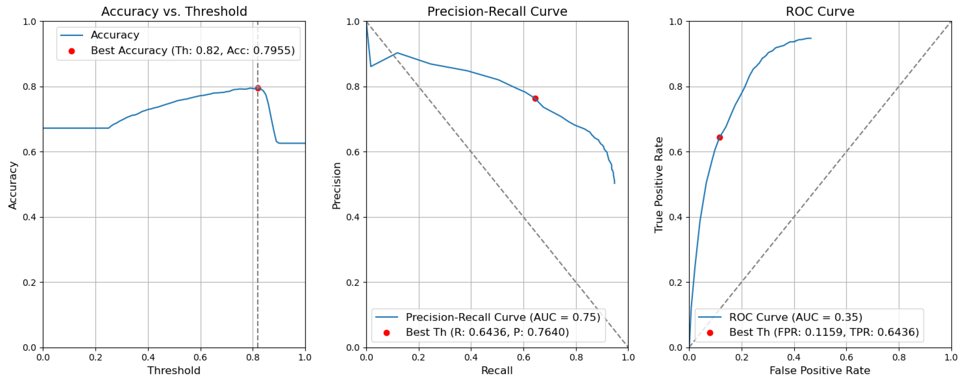
- CBAM Type II with fusion. Figure 12 illustrates the selection of different threshold values (from 0.0 to 1.0) for all elementary detectors of the Type-II CBAM architecture for defects and context elements. These results are obtained after the application of the fusion rules described in Section 3.5. For elementary detectors with fusion, using the threshold value of 0.82, the resulting accuracy (Acc) is 0.7955. The precision (P) value is 0.7640. The recall (R) or true-positive rate (TPR) is equal to 0.6436. The false-positive rate (FPR) is equal to 0.1159.
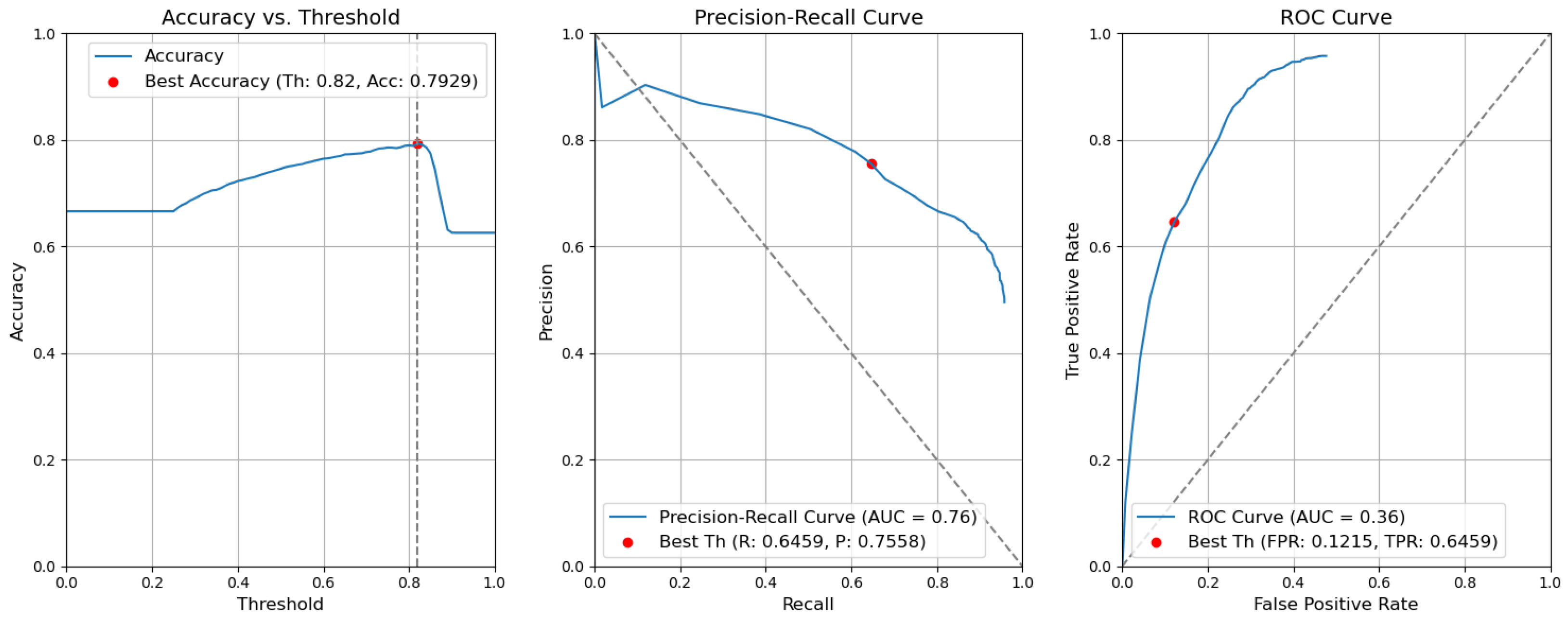
- CBAM Type II. The results obtained without applying the rules are illustrated in Figure 13. After removing the fusion rules, the accuracy was decreased by 0.0026 and is 0.7929. This is due to the slight decrease in precision (by 0.0082), which is 0.7558, and to the rise in FPR (by 0.0056 and is 0.1215). Consequently, the recall or true-positive rate value increased by 0.0023 and is equal to 0.6459.
- CBAM Type I with fusion. Using the threshold value of 0.78, the resulting accuracy (Acc) is 0.7948. The precision (P) value is 0.6935. The recall (R) or true-positive rate (TPR) is equal to 0.7773. The false-positive rate (FPR) is equal to 0.1953. Figure 14 illustrates these results.
- CBAM Type I. Without applying the rules, the accuracy decreased by 0.0059 and is 0.7889. The precision decreased by 0.0153 and is equal to 0.6782. The false-positive rate increased by 0.0139 and is equal to 0.2092. The recall or true-positive rate also increased by 0.0082 and is equal to 0.7855. We can find these results in Figure 15.
- Baseline with fusion. Using the threshold value of 0.80, the resulting accuracy (Acc) is 0.8032. The precision (P) value is 0.7122. The recall (R) or true-positive rate (TPR) is equal to 0.7698. The false-positive rate (FPR) is equal to 0.1777. Figure 16 illustrates these results.
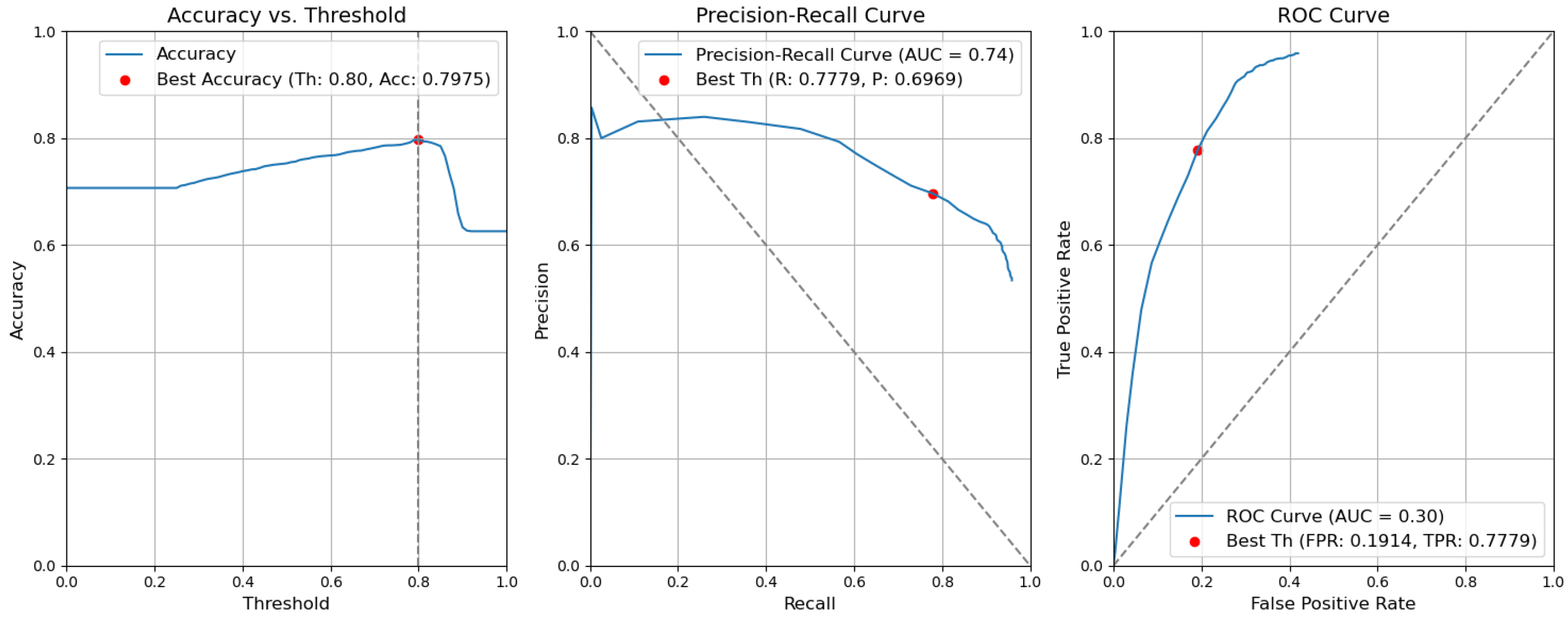
- Baseline. Without applying the rules, the accuracy decreased by 0.0057 and is 0.7975. The precision decreased by 0.0153 and is equal to 0.6969. The false-positive rate increased by 0.0137 and is equal to 0.1914. The recall or true-positive rate also increased by 0.0081 and is equal to 0.7779. We can find these results in Figure 17.
5.3. Robustness Analysis
5.4. Comparison with the State of the Art
5.5. Complexity Analysis
6. Conclusions
Author Contributions
Funding
Institutional Review Board Statement
Informed Consent Statement
Data Availability Statement
Acknowledgments
Conflicts of Interest
References
- De Melo, A.L.O.; Kaewunruen, S.; Papaelias, M.; Bernucci, L.L.B.; Motta, R. Methods to Monitor and Evaluate the Deterioration of Track and Its Components in a Railway In-Service: A Systemic Review. Front. Built Environ. 2020, 6, 118. [Google Scholar] [CrossRef]
- Yunjie, Z.; Xiaorong, G.; Lin, L.; Yongdong, P.; Chunrong, Q. Simulation of Laser Ultrasonics for Detection of Surface-Connected Rail Defects. J. Nondestruct. Eval. 2017, 36, 70. [Google Scholar] [CrossRef]
- Yuan, F.; Yu, Y.; Liu, B.; Li, L. Investigation on optimal detection position of DC electromagnetic NDT in crack characterization for high-speed rail track. In Proceedings of the 2019 IEEE International Instrumentation and Measurement Technology Conference (I2MTC), Auckland, New Zealand, 20–23 May 2019; pp. 1–6. [Google Scholar] [CrossRef]
- Lay-Ekuakille, A.; Fabbiano, L.; Vacca, G.; Kitoko, J.K.; Kulapa, P.B.; Telesca, V. A Comparison between the Decimated Padé Approximant and Decimated Signal Diagonalization Methods for Leak Detection in Pipelines Equipped with Pressure Sensors. Sensors 2018, 18, 1810. [Google Scholar] [CrossRef] [PubMed]
- Rivero, A. Data Analysis for Railway Monitoring: Artificial Intelligence to Serve the Railway Sector. Ph.D. Thesis, These de doctorat dirigee par Vanheeghe, Philippe et Duflos, Emmanuel Automatique, Genie Informatique, Traitement du Signal et des Images Centrale Lille Institut, Lille, France, 2021. [Google Scholar]
- Vieux, R.; Domenger, J.; Benois-Pineau, J.; Braquelaire, A.J. Image classification with user defined ontology. In Proceedings of the 15th European Signal Processing Conference, EUSIPCO 2007, Poznan, Poland, 3–7 September 2007; pp. 723–727. [Google Scholar]
- González-Díaz, I.; Buso, V.; Benois-Pineau, J. Perceptual modeling in the problem of active object recognition in visual scenes. Pattern Recognit. 2016, 56, 129–141. [Google Scholar] [CrossRef]
- Mallick, R.; Yebda, T.; Benois-Pineau, J.; Zemmari, A.; Pech, M.; Amieva, H. Detection of Risky Situations for Frail Adults With Hybrid Neural Networks on Multimodal Health Data. IEEE Multim. 2022, 29, 7–17. [Google Scholar] [CrossRef]
- Jocher, G. Ultralytics YOLOv5. Available online: https://github.com/ultralytics/yolov5 (accessed on 20 October 2023).
- Krizhevsky, A.; Sutskever, I.; Hinton, G.E. ImageNet Classification with Deep Convolutional Neural Networks. Commun. ACM 2017, 60, 84–90. [Google Scholar] [CrossRef]
- Wang, W.; Dai, J.; Chen, Z.; Huang, Z.; Li, Z.; Zhu, X.; Hu, X.; Lu, T.; Lu, L.; Li, H.; et al. InternImage: Exploring Large-Scale Vision Foundation Models with Deformable Convolutions. In Proceedings of the 2023 IEEE/CVF Conference on Computer Vision and Pattern Recognition (CVPR), Los Alamitos, CA, USA, 18–22 June 2023; pp. 14408–14419. [Google Scholar] [CrossRef]
- Varga, L.A.; Kiefer, B.; Messmer, M.; Zell, A. SeaDronesSee: A Maritime Benchmark for Detecting Humans in Open Water. In Proceedings of the 2022 IEEE/CVF Winter Conference on Applications of Computer Vision (WACV), Waikoloa, HI, USA, 3–8 January 2022; pp. 3686–3696. [Google Scholar] [CrossRef]
- Chen, X.; Liang, C.; Huang, D.; Real, E.; Wang, K.; Liu, Y.; Pham, H.; Dong, X.; Luong, T.; Hsieh, C.J.; et al. Symbolic Discovery of Optimization Algorithms. arXiv 2023, arXiv:2302.06675. [Google Scholar] [CrossRef]
- Wang, P.; Wang, S.; Lin, J.; Bai, S.; Zhou, X.; Zhou, J.; Wang, X.; Zhou, C. ONE-PEACE: Exploring One General Representation Model Toward Unlimited Modalities. arXiv 2023, arXiv:2305.11172. [Google Scholar] [CrossRef]
- Cumbajin, E.; Rodrigues, N.; Costa, P.; Miragaia, R.; Frazão, L.; Costa, N.; Fernández-Caballero, A.; Carneiro, J.; Buruberri, L.H.; Pereira, A. A Systematic Review on Deep Learning with CNNs Applied to Surface Defect Detection. J. Imaging 2023, 9, 193. [Google Scholar] [CrossRef]
- Girshick, R.; Donahue, J.; Darrell, T.; Malik, J. Rich feature hierarchies for accurate object detection and semantic segmentation. In Proceedings of the IEEE Conference on Computer Vision and Pattern Recognition, Columbus, OH, USA, 23–28 June 2014; pp. 580–587. [Google Scholar] [CrossRef]
- He, K.; Zhang, X.; Ren, S.; Sun, J. Spatial pyramid pooling in deep convolutional networks for visual recognition. IEEE Trans. Pattern Anal. Mach. Intell. 2015, 37, 1904–1916. [Google Scholar] [CrossRef]
- Girshick, R. Fast r-cnn. In Proceedings of the IEEE International Conference on Computer Vision, Santiago, Chile, 7–13 December 2015; pp. 1440–1448. [Google Scholar] [CrossRef]
- Dai, J.; Li, Y.; He, K.; Sun, J. R-fcn: Object detection via region-based fully convolutional networks. Adv. Neural Inf. Process. Syst. 2016, 29, 379–387. [Google Scholar] [CrossRef]
- He, K.; Gkioxari, G.; Dollár, P.; Girshick, R. Mask r-cnn. In Proceedings of the IEEE International Conference on Computer Vision, Venice, Italy, 22–29 October 2017; pp. 2961–2969. [Google Scholar] [CrossRef]
- Fan, J.; Liu, Y.; Hu, Z.; Zhao, Q.; Shen, L.; Zhou, X. Solid wood panel defect detection and recognition system based on faster R-CNN. J. For. Eng. 2019, 4, 112–117. [Google Scholar] [CrossRef]
- Ji, W.; Meng, D.; Wei, P.; Jie, X. Research on gear appearance defect recognition based on improved faster R-CNN. J. Syst. Simul. 2019, 31, 2198–2205. [Google Scholar] [CrossRef]
- Yuyan, Z.; Yongbao, L.; Yintang, W.; Zhiwei, Z. Internal defect detection of metal three-dimensional multi-layer lattice structure based on faster R-CNN. Acta Armamentarii 2019, 40, 2329. [Google Scholar] [CrossRef]
- Wen-ming, G.; Kai, L.; Hui-Fan, Q. Welding defect detection of x-ray images based on faster r-cnn model. J. Beijing Univ. Posts Telecommun. 2019, 42, 20. [Google Scholar] [CrossRef]
- Wang, J.Y.; Duan, X. Linmao Surface defect detection of inner groove in plunger brake master cylinder based on LabVIEW and Mask R-CNN. Mod. Manuf. Eng. 2020, 5, 125–132. [Google Scholar]
- Biao, C.; Kuan, S.; Jinlei, F.; Lize, Z. Research on defect detection of X-ray DR images of casting based on Mask R-CNN. Chin. J. Sci. Instrum. 2020, 41, 63–71. [Google Scholar]
- Redmon, J.; Divvala, S.; Girshick, R.; Farhadi, A. You only look once: Unified, real-time object detection. In Proceedings of the Conference on Computer Vision and Pattern Recognition, Las Vegas, NV, USA, 27–30 June 2016; pp. 779–788. [Google Scholar] [CrossRef]
- Liu, W.; Anguelov, D.; Erhan, D.; Szegedy, C.; Reed, S.; Fu, C.Y.; Berg, A.C. Ssd: Single shot multibox detector. In Proceedings of the Computer Vision–ECCV 2016: 14th European Conference, Amsterdam, The Netherlands, 11–14 October 2016; Springer International Publishing: Berlin, Germany, 2016; pp. 21–37. [Google Scholar] [CrossRef]
- Law, H.; Deng, J. CornerNet: Detecting Objects as Paired Keypoints. In Proceedings of the European Conference on Computer Vision (ECCV) 2020, Glasgow, UK, 23–28 August 2020; Volume 128, pp. 642–656. [Google Scholar] [CrossRef]
- Tan, M.; Pang, R.; Le, Q.V. EfficientDet: Scalable and Efficient Object Detection. In Proceedings of the 2020 IEEE/CVF Conference on Computer Vision and Pattern Recognition (CVPR), Los Alamitos, CA, USA, 13–19 June 2020; pp. 10778–10787. [Google Scholar] [CrossRef]
- Redmon, J.; Farhadi, A. YOLOv3: An Incremental Improvement. arXiv 2018, arXiv:1804.02767. [Google Scholar] [CrossRef]
- Jocher, G.; Chaurasia, A.; Qiu, J. Ultralytics YOLOv8. Available online: https://github.com/ultralytics/ultralytics (accessed on 20 October 2023).
- Jing, J.; Zhuo, D.; Zhang, H.; Liang, Y.; Zheng, M. Fabric defect detection using the improved YOLOv3 model. J. Eng. Fibers Fabr. 2020, 15, 1558925020908268. [Google Scholar] [CrossRef]
- Li, J.; Gu, J.; Huang, Z.; Wen, J. Application Research of Improved YOLO V3 Algorithm in PCB Electronic Component Detection. Appl. Sci. 2019, 9, 750. [Google Scholar] [CrossRef]
- Huang, R.; Gu, J.; Sun, X.; Hou, Y.; Uddin, S. A Rapid Recognition Method for Electronic Components Based on the Improved YOLO-V3 Network. Electronics 2019, 8, 825. [Google Scholar] [CrossRef]
- Du, Y.; Pan, N.; Xu, Z.; Deng, F.; Shen, Y.; Kang, H. Pavement distress detection and classification based on YOLO network. Int. J. Pavement Eng. 2021, 22, 1659–1672. [Google Scholar] [CrossRef]
- Jordan, M.I. (Ed.) Learning in Graphical Models; MIT Press: Cambridge, MA, USA, 1999. [Google Scholar] [CrossRef]
- Martínez, H.P.; Yannakakis, G.N. Deep Multimodal Fusion: Combining Discrete Events and Continuous Signals. In Proceedings of the 16th International Conference on Multimodal Interaction, New York, NY, USA, 12–26 November 2014; pp. 34–41. [Google Scholar] [CrossRef]
- Ramachandram, D.; Taylor, G.W. Deep multimodal learning: A survey on recent advances and trends. IEEE Signal Process. Mag. 2017, 34, 96–108. [Google Scholar] [CrossRef]
- Simonyan, K.; Zisserman, A. Two-stream convolutional networks for action recognition in videos. Adv. Neural Inf. Process. Syst. 2014, 27, 568–576. [Google Scholar]
- Wu, D.; Pigou, L.; Kindermans, P.J.; Le, N.D.H.; Shao, L.; Dambre, J.; Odobez, J.M. Deep Dynamic Neural Networks for Multimodal Gesture Segmentation and Recognition. IEEE Trans. Pattern Anal. Mach. Intell. 2016, 38, 1583–1597. [Google Scholar] [CrossRef] [PubMed]
- Kahou, S.E.; Pal, C.; Bouthillier, X.; Froumenty, P.; Gülçehre, c.; Memisevic, R.; Vincent, P.; Courville, A.; Bengio, Y.; Ferrari, R.C.; et al. Combining Modality Specific Deep Neural Networks for Emotion Recognition in Video. In Proceedings of the 15th ACM on International Conference on Multimodal Interaction, New York, NY, USA, 9–13 December 2013; pp. 543–550. [Google Scholar] [CrossRef]
- Bourroux, L.; Benois-Pineau, J.; Bourqui, R.; Giot, R. Multi Layered Feature Explanation Method for Convolutional Neural Networks. In Proceedings of the International Conference on Pattern Recognition and Artificial Intelligence (ICPRAI), Paris, France, 1–3 June 2022. [Google Scholar] [CrossRef]
- Ultralytics. YOLOv5: A State-of-the-Art Real-Time Object Detection System. Available online: https://docs.ultralytics.com (accessed on 31 December 2021).
- Woo, S.; Park, J.; Lee, J.Y.; Kweon, I.S. Cbam: Convolutional block attention module. In Proceedings of the European Conference on Computer Vision (ECCV), Munich, Germany, 8–14 September 2018; pp. 3–19. [Google Scholar] [CrossRef]
- Bochkovskiy, A.; Wang, C.Y.; Liao, H.Y.M. YOLOv4: Optimal Speed and Accuracy of Object Detection. arXiv 2020, arXiv:2004.10934. [Google Scholar] [CrossRef]
- Wang, C.Y.; Liao, H.Y.M.; Wu, Y.H.; Chen, P.Y.; Hsieh, J.W.; Yeh, I.H. CSPNet: A new backbone that can enhance learning capability of CNN. In Proceedings of the IEEE/CVF Conference on Computer Vision and Pattern Recognition Workshops, Seattle, WA, USA, 14–19 June 2020; pp. 390–391. [Google Scholar] [CrossRef]
- He, K.; Zhang, X.; Ren, S.; Sun, J. Deep Residual Learning for Image Recognition. In Proceedings of the 2016 IEEE Conference on Computer Vision and Pattern Recognition (CVPR), Las Vegas, NV, USA, 26 June–1 July 2016; pp. 770–778. [Google Scholar] [CrossRef]
- Obeso, A.M.; Benois-Pineau, J.; García Vázquez, M.S.; Álvaro Ramírez Acosta, A. Visual vs internal attention mechanisms in deep neural networks for image classification and object detection. Pattern Recognit. 2022, 123, 108411. [Google Scholar] [CrossRef]
- Hu, J.; Shen, L.; Sun, G. Squeeze-and-Excitation Networks. In Proceedings of the 2018 IEEE/CVF Conference on Computer Vision and Pattern Recognition, Salt Lake City, UT, USA, 18–23 June 2018; pp. 7132–7141. [Google Scholar] [CrossRef]
- Chen, Y.; Kalantidis, Y.; Li, J.; Yan, S.; Feng, J. A2-Nets: Double attention networks. In Proceedings of the 32nd International Conference on Neural Information Processing Systems, Red Hook, NY, USA, 3–8 December 2018; pp. 350–359. [Google Scholar] [CrossRef]
- Zeiler, M.D.; Fergus, R. Visualizing and Understanding Convolutional Networks. In Proceedings of the Computer Vision—ECCV 2014, Zurich, Switzerland, 6–12 September 2014; Fleet, D., Pajdla, T., Schiele, B., Tuytelaars, T., Eds.; Springer International Publishing: Cham, Switzerland, 2014; pp. 818–833. [Google Scholar] [CrossRef]
- Zhou, B.; Khosla, A.; Lapedriza, A.; Oliva, A.; Torralba, A. Learning deep features for discriminative localization. In Proceedings of the IEEE Conference on Computer Vision and Pattern Recognition, Las Vegas, NV, USA, 27–30 June 2016; pp. 2921–2929. [Google Scholar] [CrossRef]
- Zagoruyko, S.; Komodakis, N. Paying more attention to attention: Improving the performance of convolutional neural networks via attention transfer. arXiv 2016, arXiv:1612.03928. [Google Scholar] [CrossRef]
- Lin, T.Y.; Maire, M.; Belongie, S.; Hays, J.; Perona, P.; Ramanan, D.; Dollár, P.; Zitnick, C.L. Microsoft COCO: Common Objects in Context. In Proceedings of the Computer Vision—ECCV 2014, Zurich, Switzerland, 6–12 September 2014; Springer International Publishing: Cham, Switzerland, 2014; pp. 740–755. [Google Scholar] [CrossRef]
- Li, H.; Wang, F.; Liu, J.; Song, H.; Hou, Z.; Dai, P. Ensemble model for rail surface defects detection. PLoS ONE 2022, 17, e0268518. [Google Scholar] [CrossRef]


| Defects Detected | Contextual Elements Detected | Decision Made by the System | ||
|---|---|---|---|---|
| Missing Nuts | Fishplate Failure | No Defect | ||
| Missing nuts | Fishplate (image) | X | ||
| CES (image) | X | |||
| Fishplate failure | Fishplate (image) | X | ||
| Class | Used Examples |
|---|---|
| Defective_fastener | 8127 |
| Surface_defect | 2679 |
| Missing_nut | 1490 |
| Total | 12,296 |
| Class | Used Examples |
|---|---|
| Braid | 3783 |
| CES | 577 |
| Fishplate | 5923 |
| Seal | 6441 |
| Welding | 2837 |
| Markings | 2820 |
| Total | 23,391 |
| (a) YOLOv5m (Baseline) and YOLOv8m (Baseline) | ||||||||
| Model Type | YOLOv5 (Baseline) | YOLOv8 (Baseline) | ||||||
| Class | P | R | mAP50* | mAP50-95* | P | R | mAP50* | mAP50-95* |
| Overall | 0.886 | 0.880 | 0.901 | 0.468 | 0.887 | 0.865 | 0.877 | 0.466 |
| Defective fastener | 0.934 | 0.962 | 0.961 | 0.632 | 0.935 | 0.960 | 0.961 | 0.644 |
| Surface defect | 0.814 | 0.764 | 0.848 | 0.340 | 0.818 | 0.720 | 0.793 | 0.326 |
| Missing nut | 0.902 | 0.916 | 0.895 | 0.431 | 0.909 | 0.916 | 0.875 | 0.427 |
| (b) YOLOv5m with CBAM at 9th Stage (Type I) and YOLOv8m with CBAM at 9th Stage (Type I) | ||||||||
| Model Type | YOLOv5 with CBAM at 9th Stage (Type I) | YOLOv8 with CBAM at 9th Stage (Type I) | ||||||
| Class | P | R | mAP50* | mAP50-95* | P | R | mAP50* | mAP50-95* |
| Overall | 0.875 | 0.887 | 0.895 | 0.455 | 0.886 | 0.867 | 0.873 | 0.464 |
| Defective fastener | 0.936 | 0.967 | 0.963 | 0.634 | 0.939 | 0.963 | 0.967 | 0.648 |
| Surface defect | 0.789 | 0.784 | 0.831 | 0.310 | 0.801 | 0.718 | 0.757 | 0.319 |
| Missing nut | 0.900 | 0.910 | 0.892 | 0.421 | 0.919 | 0.921 | 0.896 | 0.426 |
| (c) YOLOv5m with CBAM at Three Scales (Type II) and YOLOv8m with CBAM at Three Scales (Type II) | ||||||||
| Model Type | YOLOv5 with CBAM at Three Scales (Type II) | YOLOv8 with CBAM at Three Scales (Type II) | ||||||
| Class | P | R | mAP50* | mAP50-95* | P | R | mAP50* | mAP50-95* |
| Overall | 0.892 | 0.895 | 0.903 | 0.469 | 0.878 | 0.879 | 0.882 | 0.469 |
| Defective fastener | 0.942 | 0.968 | 0.965 | 0.633 | 0.926 | 0.964 | 0.967 | 0.651 |
| Surface defect | 0.832 | 0.795 | 0.840 | 0.361 | 0.795 | 0.752 | 0.800 | 0.330 |
| Missing nut | 0.910 | 0.921 | 0.904 | 0.413 | 0.914 | 0.921 | 0.880 | 0.425 |
| (a) YOLOv5m (Baseline) and YOLOv8m (Baseline) | ||||||||
| Model Type | YOLOv5 (Baseline) | YOLOv8 (Baseline) | ||||||
| Class | P | R | mAP50* | mAP50-95* | P | R | mAP50* | mAP50-95* |
| Overall | 0.893 | 0.932 | 0.923 | 0.492 | 0.902 | 0.942 | 0.926 | 0.493 |
| Braid | 0.880 | 0.953 | 0.928 | 0.530 | 0.898 | 0.964 | 0.963 | 0.574 |
| CES | 0.918 | 0.983 | 0.984 | 0.558 | 0.940 | 0.974 | 0.976 | 0.558 |
| Fishplate | 0.932 | 0.936 | 0.968 | 0.627 | 0.920 | 0.957 | 0.953 | 0.559 |
| Seal | 0.859 | 0.877 | 0.848 | 0.329 | 0.866 | 0.876 | 0.864 | 0.349 |
| Welding | 0.906 | 0.943 | 0.916 | 0.441 | 0.913 | 0.953 | 0.912 | 0.443 |
| Markings | 0.860 | 0.938 | 0.886 | 0.470 | 0.875 | 0.927 | 0.887 | 0.473 |
| (b) YOLOv5m with CBAM at 9th Stage (Type I) and YOLOv8m with CBAM at 9th Stage (Type I) | ||||||||
| Model Type | YOLOv5 with CBAM at 9th Stage (Type I) | YOLOv8 with CBAM at 9th Stage (Type I) | ||||||
| Class | P | R | mAP50* | mAP50-95* | P | R | mAP50* | mAP50-95* |
| Overall | 0.891 | 0.939 | 0.918 | 0.489 | 0.904 | 0.939 | 0.932 | 0.517 |
| Braid | 0.878 | 0.953 | 0.926 | 0.528 | 0.892 | 0.958 | 0.957 | 0.574 |
| CES | 0.920 | 0.974 | 0.981 | 0.554 | 0.934 | 0.969 | 0.975 | 0.575 |
| Fishplate | 0.930 | 0.940 | 0.962 | 0.624 | 0.947 | 0.978 | 0.984 | 0.679 |
| Seal | 0.861 | 0.874 | 0.841 | 0.325 | 0.865 | 0.860 | 0.862 | 0.351 |
| Welding | 0.901 | 0.954 | 0.912 | 0.440 | 0.915 | 0.951 | 0.920 | 0.445 |
| Markings | 0.856 | 0.940 | 0.889 | 0.466 | 0.870 | 0.918 | 0.895 | 0.477 |
| (c) YOLOv5m with CBAM at Three Scales (Type II) and YOLOv8m with CBAM at Three Scales (Type II) | ||||||||
| Model Type | YOLOv5 with CBAM at Three Scales (Type II) | YOLOv8 with CBAM at Three Scales (Type II) | ||||||
| Class | P | R | mAP50* | mAP50-95* | P | R | mAP50* | mAP50-95* |
| Overall | 0.901 | 0.941 | 0.924 | 0.493 | 0.899 | 0.935 | 0.923 | 0.495 |
| Braid | 0.900 | 0.955 | 0.933 | 0.515 | 0.893 | 0.962 | 0.954 | 0.578 |
| CES | 0.924 | 0.983 | 0.986 | 0.561 | 0.940 | 0.974 | 0.969 | 0.569 |
| Fishplate | 0.939 | 0.941 | 0.963 | 0.628 | 0.916 | 0.946 | 0.949 | 0.563 |
| Seal | 0.868 | 0.878 | 0.848 | 0.330 | 0.862 | 0.862 | 0.865 | 0.450 |
| Welding | 0.914 | 0.955 | 0.925 | 0.454 | 0.908 | 0.946 | 0.906 | 0.439 |
| Markings | 0.861 | 0.942 | 0.894 | 0.469 | 0.876 | 0.922 | 0.892 | 0.474 |
| Architecture | ||||||
|---|---|---|---|---|---|---|
| Metric | Type II + Fusion | Type II | Type I + Fusion | Type I | Baseline + Fusion | Baseline |
| Acc | 0.7955 | 0.7929 | 0.7948 | 0.7889 | 0.8032 | 0.7975 |
| P | 0.7640 | 0.7558 | 0.6935 | 0.6782 | 0.7122 | 0.6969 |
| R or TPR | 0.6436 | 0.6459 | 0.7773 | 0.7855 | 0.7698 | 0.7779 |
| FPR | 0.1159 | 0.1215 | 0.1953 | 0.2092 | 0.1777 | 0.1914 |
| Baseline + Fusion | Baseline | |||||||
|---|---|---|---|---|---|---|---|---|
| Acc | P | R | FPR | Acc | P | R | FPR | |
| −30 | 0.8024 | 0.7152 | 0.7593 | 0.1730 | 0.7967 | 0.6999 | 0.7663 | 0.1861 |
| −20 | 0.8006 | 0.7115 | 0.7599 | 0.1761 | 0.7949 | 0.6964 | 0.7669 | 0.1892 |
| −10 | 0.8013 | 0.7110 | 0.7640 | 0.1773 | 0.7961 | 0.6964 | 0.7721 | 0.1904 |
| 0 | 0.8032 | 0.7122 | 0.7698 | 0.1777 | 0.7975 | 0.6969 | 0.7779 | 0.1914 |
| +10 | 0.8016 | 0.7089 | 0.7703 | 0.1806 | 0.7959 | 0.6940 | 0.7776 | 0.1940 |
| +20 | 0.8010 | 0.7263 | 0.7297 | 0.1580 | 0.7965 | 0.7140 | 0.7343 | 0.1680 |
| +30 | 0.8003 | 0.7241 | 0.7308 | 0.1598 | 0.7958 | 0.7119 | 0.7355 | 0.1698 |
| Type I + Fusion | Type I | |||||||
|---|---|---|---|---|---|---|---|---|
| Acc | P | R | FPR | Acc | P | R | FPR | |
| −30 | 0.7964 | 0.6873 | 0.8023 | 0.2070 | 0.7903 | 0.6723 | 0.8110 | 0.2213 |
| −20 | 0.7936 | 0.6836 | 0.8000 | 0.2100 | 0.7878 | 0.6786 | 0.7797 | 0.2077 |
| −10 | 0.7957 | 0.6965 | 0.7738 | 0.1919 | 0.7900 | 0.6812 | 0.7826 | 0.2059 |
| 0 | 0.7948 | 0.6935 | 0.7773 | 0.1953 | 0.7889 | 0.6782 | 0.7855 | 0.2092 |
| +10 | 0.7949 | 0.6938 | 0.7772 | 0.1951 | 0.7888 | 0.6782 | 0.7855 | 0.2090 |
| +20 | 0.7946 | 0.6937 | 0.7767 | 0.1952 | 0.7892 | 0.7298 | 0.6738 | 0.1442 |
| +30 | 0.7932 | 0.6923 | 0.7733 | 0.1954 | 0.7877 | 0.7500 | 0.6331 | 0.1226 |
| Type II + Fusion | Type II | |||||||
|---|---|---|---|---|---|---|---|---|
| Acc | P | R | FPR | Acc | P | R | FPR | |
| −30 | 0.7954 | 0.7120 | 0.7372 | 0.1712 | 0.7924 | 0.7590 | 0.6390 | 0.1182 |
| −20 | 0.7956 | 0.7107 | 0.7413 | 0.1732 | 0.7920 | 0.7562 | 0.6419 | 0.1206 |
| −10 | 0.7950 | 0.7636 | 0.6424 | 0.1160 | 0.7925 | 0.7554 | 0.6448 | 0.1215 |
| 0 | 0.7955 | 0.7640 | 0.6436 | 0.1159 | 0.7929 | 0.7558 | 0.6459 | 0.1215 |
| +10 | 0.7953 | 0.7627 | 0.6448 | 0.1169 | 0.7931 | 0.7556 | 0.6471 | 0.1219 |
| +20 | 0.7951 | 0.6936 | 0.7791 | 0.1958 | 0.7933 | 0.7785 | 0.6151 | 0.1025 |
| +30 | 0.7942 | 0.7608 | 0.6436 | 0.1180 | 0.7923 | 0.7757 | 0.6151 | 0.1040 |
| Baseline (Object) | Baseline (Context) | CBAM Type I (Object) | CBAM Type I (Context) | CBAM Type II (Object) | CBAM Type II (Context) | |
|---|---|---|---|---|---|---|
| Training time (h) | 8.1 | 10 | 7.8 | 9.7 | 10 | 12.4 |
| Inference speed (s): image resolution (774 × 1480) | 0.0090 | 0.0090 | 0.0085 | 0.0085 | 0.0113 | 0.0113 |
| Inference speed (s): image resolution (1508 × 1500) | 0.0124 | 0.0124 | 0.0119 | 0.0119 | 0.0158 | 0.0158 |
| No. of parameters | 20,861,016 | 20,873,139 | 17,319,098 | 17,331,221 | 21,480,702 | 21,489,369 |
| Model size (MB) | 40.1 | 40.2 | 33.3 | 33.4 | 41.3 | 41.3 |
Disclaimer/Publisher’s Note: The statements, opinions and data contained in all publications are solely those of the individual author(s) and contributor(s) and not of MDPI and/or the editor(s). MDPI and/or the editor(s) disclaim responsibility for any injury to people or property resulting from any ideas, methods, instructions or products referred to in the content. |
© 2024 by the authors. Licensee MDPI, Basel, Switzerland. This article is an open access article distributed under the terms and conditions of the Creative Commons Attribution (CC BY) license (https://creativecommons.org/licenses/by/4.0/).
Share and Cite
Zhukov, A.; Rivero, A.; Benois-Pineau, J.; Zemmari, A.; Mosbah, M. A Hybrid System for Defect Detection on Rail Lines through the Fusion of Object and Context Information. Sensors 2024, 24, 1171. https://doi.org/10.3390/s24041171
Zhukov A, Rivero A, Benois-Pineau J, Zemmari A, Mosbah M. A Hybrid System for Defect Detection on Rail Lines through the Fusion of Object and Context Information. Sensors. 2024; 24(4):1171. https://doi.org/10.3390/s24041171
Chicago/Turabian StyleZhukov, Alexey, Alain Rivero, Jenny Benois-Pineau, Akka Zemmari, and Mohamed Mosbah. 2024. "A Hybrid System for Defect Detection on Rail Lines through the Fusion of Object and Context Information" Sensors 24, no. 4: 1171. https://doi.org/10.3390/s24041171