1. Introduction
The multilevel inverter is a power electronic device that generates output voltage waveforms and current waveforms using a variety of direct current (DC) voltage sources and power switches [
1]. Multilevel inverters are widely used in low-voltage situations and mid-frequency switching frequency scenarios due to their advantages of low switching transient voltage change rate, small harmonic distortion, and high power conversion efficiency [
2], and have become indispensable electronic devices in power systems as modern industry develops in the direction of scale, accuracy, systematization, automation, and intelligence. The complexity of the T-type topology and the abundance of power semiconductor devices have recently raised questions about the ability of the system to operate reliably in comparison to the traditional two-level inverter [
3].
Because semiconductor power devices are relatively fragile, open-circuit (OC) faults and short-circuit (SC) faults of insulated gate bipolar transistors (IGBTs) can be distinguished based on their external behavior [
4]. SC faults cause short circuits and abnormal overcurrent states, causing other components to be damaged. It is necessary to isolate the problematic component or to immediately shut down the whole system, for instance, using desaturation detection in the door driver or fast fuses [
5]. On the contrary, OC fault may not immediately cause system failure but may cause current distortion and secondary damage to other components due to increased noise and voltage stress. As a result, effective OC fault diagnosis is critical for improving power system reliability.
At present, more methods based on signal processing are being developed to decompose, convert, or lower the dimension of system detection data according to the signal analysis strategy and extract feature information from it. Fault diagnosis and identification are achieved by comparing the changing pattern of feature information before and after the fault. The authors in [
6] proposed a non-invasive diagnostic strategy to detect the near-field voltage signal of the inverter DC bus through the antenna and extract the spectral features of the collected signal using fast Fourier transform (FFT) as a basis for fault classification. However, due to the limitation of the amount of diagnostic information, this method can only achieve the diagnosis of the clamping diode open-circuit fault. A discrete wavelet transform-based fault feature extraction strategy for microgrid inverters was proposed by the authors in [
7]. The authors in [
8] propose a fault-diagnosis method based on the average modulation voltage model for multi-current sensor disordered grid-connected inverters, which establishes the average modulation voltage model of three-phase steady-state coordinates and estimates the difference between the measured value and the actual value of the current by the model. Then, the fault is found. The experimental results show that the method can accurately locate the fault and perform fault-tolerant control when multiple sensors have offset faults at the same time. By symmetrically reconstructing the phase current signal, the effect of load variation is eliminated while retaining the main features of the fault. Then, multi-scale feature extraction is performed on the signal, and the energy coefficients of each group of current signals at different frequencies obtained are used as diagnostic classification information. However, the selection of wavelet bases will directly affect the extraction effect of fault features, which increases the difficulty of applying this method. To accurately detect IGBT switching faults, a new method based on an enhanced version of the variable mode decomposition algorithm (EVMD) combined with wavelet packet analysis (WPA) and scalar indicators is proposed by the authors in [
9] to detect OC faults, which also shows how effective the suggested method is at diagnosing OC faults. For three-level active neutral-point-clamped (3LANPC) inverters, the authors in [
10] established a predictive current model and seamlessly integrated the residuals of the predicted current vectors between the measured and predicted currents into the backward optimization of the MPC to diagnose inverter faults, which reduces the complexity of inverter fault identification, while the authors defined the counting function within each current cycle, which enhances the robustness of the algorithm. However, the method proposed in the article was based on generalized current residuals and a fault hypothesis prediction model. In [
11], a method based on an average voltage vector was proposed, in which the threshold value is established by vector trajectory prediction, and the diagnostic variables include neutral point potential, eigenvector angle, and eigenvector modulus. These methods, however, all rely on signals provided by the system controller, resulting in a lengthy diagnosis time. To address this issue, the authors in [
12] proposed using simple logic circuits to process the voltage and switching signals of the upper bridge transistors, as well as adding hardware to the inverter to provide transient fault information, but this introduced additional costs and complexity. Following that, a model simulation that infers system operation is proposed. For example, consider the hybrid logic dynamic diagnosis model, which is made up of a two-level inverter and an NPC inverter [
13,
14]. The diagnostic signal is defined as the difference between the sampling and estimated currents, and the fault location is determined by the residual change rate. In [
15], branch level and equipment level faults are identified hierarchically using the DC-link model, and parameter errors like inductance error and sampling error are processed to ensure accurate diagnosis results while also enhancing diagnosis speed and robustness. However, OC faults in different inverter transistors can produce similar fault characteristics [
16].
Some artificial intelligence methods are used for state feature classification and are becoming a prominent research area as machine-learning (ML) technology and computing capacity grow. The authors in [
17] made improvements to convolutional neural networks using a global average pooling layer instead of a fully connected layer, and the improved method reduces the number of model parameters of traditional neural networks greatly, which is beneficial to achieving fast fault diagnosis of inverters. To further optimize the diagnostic performance and improve diagnostic accuracy, its integrated processing and collaborative analysis are used for inverter fault diagnosis, which is a common information fusion process. The combination of different algorithms is used to enhance the extraction of fault feature information and to improve the classification and discrimination of fault features at the same time. The authors in [
18] carried out data processing and model construction for inverter open-circuit faults. In order to increase the number of samples, the authors used a Conditional Variational Auto-Encoder for data enhancement of the fault samples and Wavelet Packet Decomposition to eliminate the noise in the samples; then, the authors constructed an improved residual network with a channel attention module as a fault-diagnosis model, and the simulation results show that targeting the inverter has higher diagnostic accuracy, faster convergence speed and shorter iteration period in fault diagnosis. However, the methodology used by the authors is more stringent on the accuracy of the dataset. Any deviation or error present in these initial fault datasets may affect the accuracy of the final fault diagnosis. The authors in [
19] proposed a neural network diagnosis strategy based on a circuit resolution model. This method combines the advantages of both circuit analysis and data-driven diagnostic strategies, derives diagnostic signals that directly reflect circuit fault patterns through the parsing model, and then uses Artificial Neural Network (ANN) to identify and classify the feature information in the diagnostic signals, avoiding complex fault analysis, rule specification, and threshold selection problems. Abdo, Ali, and colleagues proposed improving fault classification accuracy by optimizing the data itself [
20]. In [
21], a long short-term memory (LSTM) neural network and a clustering algorithm were used to create a neural network model for fault detection. To locate faults, the authors in [
22] combined a deep convolutional network with network topology. Zhou et al. then used a granular Markov model to detect anomalous behavior after being inspired by the thought of information granularity [
23]. For neutral-point-clamped inverters, the authors in [
24] proposed a data-driven inverter fault-diagnosis method based on the design of labels to simplify the traditional labeling method and one-dimensional depth-separable convolution (1D-DSC) and global maximum pooling (GMP) methods to process the data. Then, the TensorRT framework is used for model compression and optimization. Simulation results show that the proposed method can reduce the number of model parameters by more than 90% and has better online application potential for fault diagnosis. The authors in [
25] combined two methods of chaotic adaptive gravity search algorithm (GSA) and back propagation neural network (BPNN) optimized by particle swarm optimization(PSO) algorithm to establish a fault-diagnosis model based on chaotic adaptive GSA-PSO-BPNN, which improved the fault classification performance, and the feasibility and effectiveness of the algorithm was demonstrated. Although the above literature does not require the analysis of the circuit operation mechanism or the creation of an accurate circuit model, the diagnosis time for faults is generally long. This is because complex calculations are generally performed on many diagnostic signals to accurately identify fault characteristics, a process that requires long data acquisition time and signal processing time.
Power inverters, on the other hand, are more complex systems, making it challenging to collect complete experimental data for fault diagnosis. Rough set theory is a new mathematical tool that can be used to deal with fuzzy and uncertain knowledge and has strong qualitative analysis capabilities. Rough sets can be directly analyzed and reasoned from experimental data to discover a large amount of implicit information knowledge and reveal the inherent law. Rough set attribute reduction has been used to help diagnose power transformer faults in recent years, with some success [
26,
27].
To summarize, artificial intelligence-based approaches may learn the nonlinear relationship between faults and fault features from data and have better diagnostic detection capabilities. However, when the neural network method is applied in the field of fault diagnosis, training samples are not easy to obtain, and it is difficult to perfectly integrate all expert experience and knowledge, making the diagnosis inaccurate and low precision. Integrated artificial intelligence and signal processing combine the advantages of different strategies. The required data are fewer, and the diagnostic model structure is relatively simple, but it still takes more than half the fundamental wave period to locate the fault. This speed is difficult to meet on some occasions that require high real-time performance of fault protection isolation or fault tolerance. In contrast, the most important feature of the rough set method is that it can objectively describe and process uncertain events without requiring subjective a priori information outside the data-set, and the core element of the method is attribute parsimony. In inverter fault diagnosis, rough set attribute simplification is usually used to reduce the dimensionality of feature quantities and reduce the size and complexity of the system. Therefore, the use of rough set theory in combination with neural networks can reduce the size of the system and decrease the time of fault diagnosis, which will achieve more desirable results in fault diagnosis.
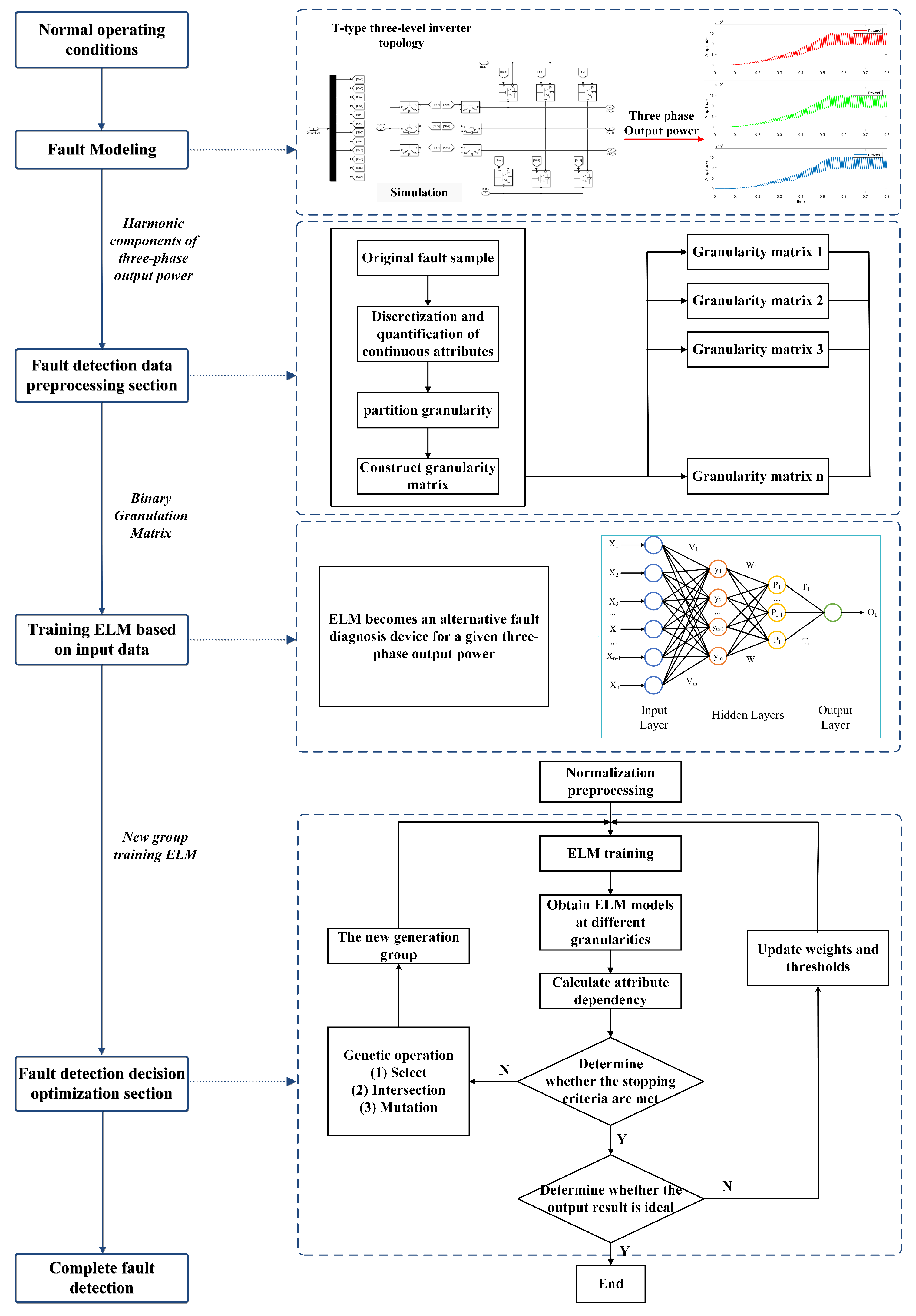
As a result, this paper processes an ELM network model for comprehensive inverter fault diagnosis using a knowledge-reduction method based on rough set (RS) theory. This paper’s main contributions are as follows: (1) Each internal IGBT operational state is determined by examining the power value changes associated with the positive and negative half-waves of each phase current of the three-level inverter. (2) A genetic algorithm (GA)-based binary granular matrix knowledge-reduction method is proposed. The decision attributes of the problem are derived through knowledge reduction under the assumption that the classification ability of the information system remains unchanged. (3) Create a fault detection model that combines GA-GrC and ELM neural networks, replace all attributes with reduction results, improve the classification performance of the ELM neural network, and thus improve the diagnosis speed, accuracy, and real-time performance of the detection system.
3. Fault Characteristic Selection
The factors influencing the occurrence of faults are complex, and the fault sample data have many attributes and large dimensions, which leads to long data-processing time and makes fault classification difficult. Furthermore, there are a significant number of similar attributes in the fault data, and these similar attributes have an approximate influence on the fault classification results, with little difference. As a result, this paper proposes a method for reducing fault attributes, in which one main attribute replaces the approximate attribute for subsequent data classification.
3.1. Knowledge-Reduction Method Based on Granular Matrix
Professor Zadeh developed the concept of granular computing (GrC) [
28]. Granular computing is a new computing paradigm that addresses difficult challenges. It uses organized thinking, structured problem-solving methodologies, and structured information processing models as research subjects. The primary idea is to use hierarchical degrees of granularity to abstract and refine complicated problems, resulting in many simpler problems to solve. Three theoretical models are highlighted: rough set, quotient space, and computing words. RS theory can analyze and express fuzzy knowledge, as well as extract hidden rules from large amounts of data for analysis and solution. Additionally, RS theory and other machine-learning algorithms are very complementary, and their combined advantages can be very beneficial.
The research object in the framework of RS theory is an information system composed of an object set and an attribute set. The information system is defined as T, i.e., . where U is the collection of objects, also known as the universe, and M and N are sets of conditional and decision attributes, respectively. V and f represent range and information function collections, respectively. A set of knowledge includes all subsets. This “attribute-value” relationship results in a collection of decision tables. When redundant or unimportant knowledge is removed from the decision information system, the information system is said to be simplified.
Granulation and granular computing are the most fundamental problems in granular computing. Granulation is the division of a problem space into several subspaces or the classification of individuals in the problem space based on useful information and knowledge. Granules are the name given to these classes. The key to granular computing is to understand how to build a reasonable granular world and solve practical problems. However, representing the concept of rough sets with binary particles is a convenient and feasible algorithm model.
Let
represent a data-set and
represent an equivalence relation on
U, denoted as
, where
. The granularity of
P is denoted as
, and its specific calculation formula is:
The particle size of
P represents its resolution. For
, when
,
u and
v are indistinguishable under
P, If it is indistinguishable, it belongs to a different
equivalence class. It can be concluded that
represents the probability of
indiscernibility of two randomly selected objects in
U, and the higher the value, the lower the resolution ability. Define the resolution
of knowledge
P as:
Because of the diversity of each piece of knowledge and the complexity of its contents, this paper uses binary particles to represent each piece of knowledge. Let be the universe and R be the equivalence relation. Each equivalence class in can be expressed by an n -bit binary string. If the bit is 0, does not belong to this granule; if it is 1, it means belongs to this granule.
3.2. Characteristic Selection
Based on the preceding understanding of the essential ideas of granular computing, this part describes the relevant operations of granules and develops the operational basis of the binary granular matrix knowledge-reduction methodology based on genetic algorithms.
The binary particle matrix is defined as
, where
is the relation matrix of the attribute set
M and
N. That is
Among them, . a and b represent the binary strings under the corresponding set.
The relation matrix , whose value corresponds to the proportion of elements in , expresses a subordinate relation between all equivalent classes and . In this manner, the chromosome of the genetic algorithm can be sequentially mapped to each attribute. Each binary string represents a chromosome, and each binary particle, which has a value range of , represents a gene.
The dependence of the attribute
describes the compatibility of the decision information system, where
In the formula, the number of elements in is represented by , the number of elements in is known as the M positive domain of N, and the total number of elements in the universe U is represented by . When , it is a compatible decision information system; otherwise, it is called an incompatible decision information system.
The set obtained after reduction is denoted as
Q, and the set of irreducible relations contained in all reduced attribute sets is referred to as core attribute, i.e., the intersection of the reduced set
, denoted as
. The collection of significant attributes required for this knowledge is referred to as the core attribute. Verify the compatibility of other knowledge with kernel attributes based on the obtained core attributes and then compute the dependency to determine the minimal set of attributes. The specific algorithm is shown in Algorithm 1.
| Algorithm 1 Attribute Reduction Algorithm |
- 1:
Input: Information System ; - 2:
Calculate : , calculate , all attributes with constitute ; - 3:
; - 4:
Determine whether is valid. If so, proceed to step 7; otherwise, proceed to step 5; - 5:
Calculate all values of , recorded as , take to satisfy: ; - 6:
, then proceed to step 4; - 7:
Output minimum reduction ;
|
Finally, the fitness function is used to search. Assume that any object
U has the conditional attribute
M, and that its fitness is as follows [
29].
where
stands for the number of genes for which conditional attribute
M has a value of 1, and
is the extent to which the decision attribute
N is dependent on the attribute subset corresponding to conditional attribute
M. It can be seen that the fitness function takes the number of subset elements and attribute dependency into account completely. Conditional attributes can be managed to evolve to the minimum attribute reduction set to achieve this.
For kernel attributes that cannot accurately describe all information, randomly select two attributes from set
U for crossover, generating two new attributes. The new individual is formed by the intersection of attribute
p and attribute
q at gene
j:
where
a is a random number of [0, 1].
Randomly select attribute
X from set
U, mutate the gene
j of that attribute, and the resulting new individual is:
where
b and
c are random numbers between [0, 1], it is the current iteration number, and
is the maximum number of iterations.
In each iteration, the best conditional attribute is preserved to prevent it from undergoing crossover and mutation again, ensuring the maximum inheritance of the conditional attribute. During each iteration, the worst attribute in the current population is replaced with the best attribute.
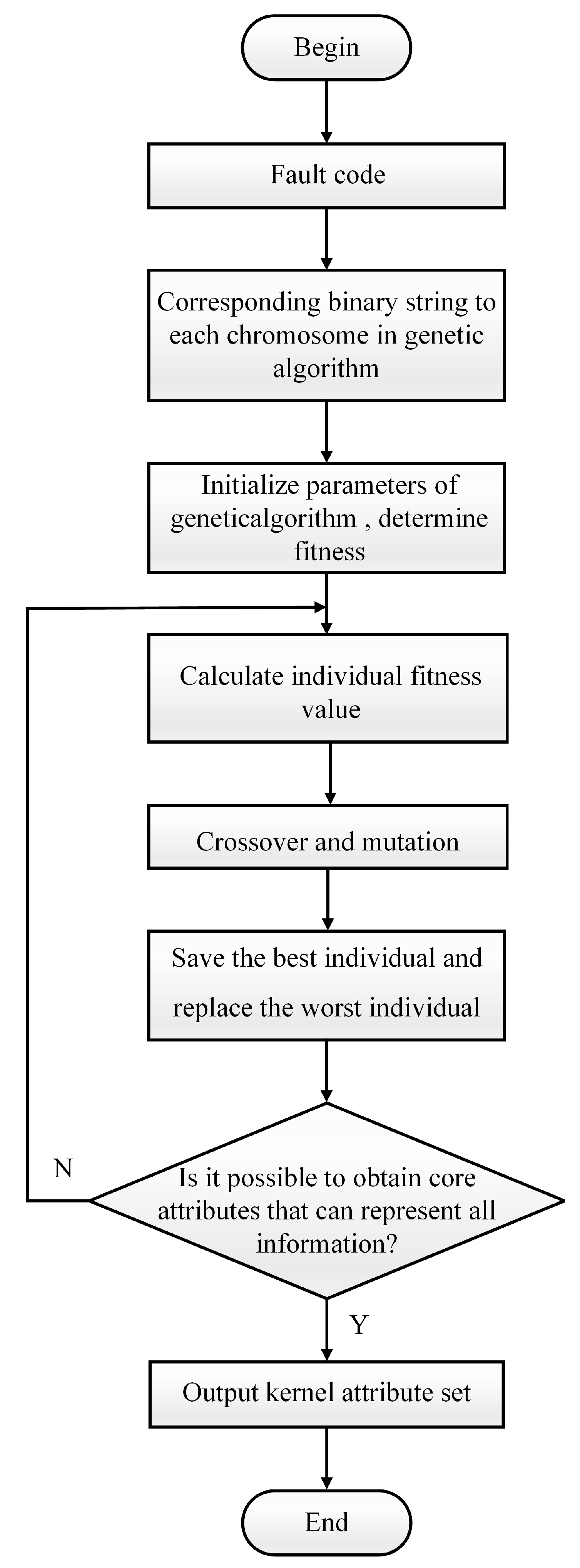
Continue the repetition until GA training reaches the maximum number of iterations, then determine the final kernel attribute set based on the fitness value.
Traditional genetic algorithms frequently use constant probabilities for crossover and mutation. As a result, the direct genetic operation of the traditional genetic algorithm on the population significantly slows convergence and fails to identify individual traits. To address this problem, this study adapts the probability values of crossover and mutation based on the population’s fitness value. This approach can improve the genetic evolutionary algorithm’s convergence speed and accuracy, as well as its global search capabilities while avoiding slipping into the local optimal solution.
Figure 5 below depicts the flow chart for the binary granulation matrix knowledge-reduction approach based on genetic algorithm optimization.
3.3. Fault Detection Model Based on GA-GrC-ELM
The ELM neural network, also known as the feedforward neural network, uses the error between the output result and the real result to estimate the error of the previous layer of the output layer and then uses the error of this layer to estimate the error of the previous layer so that the error estimate of each layer is obtained repeatedly. The parameters of the ELM hidden layer can be set randomly, or a kernel function can be used as the hidden layer. ELM can only determine the output weight by computing the inverse of the parameter matrix
H. The training process goes as follows:
In this formula,
represents the weight from the input layer to the hidden layer,
represents the system bias,
represents the weight from the hidden layer to the output layer,
g represents the activation function,
n represents the size of the training set,
represents the output value, i.e., the classification result. To infinitely approximate the real result of the training data, the classification result is consistent with the real result
P, i.e.,
, so the formula can be obtained
Written in matrix form as
H is the output matrix of the hidden layer. The specific form is as follows:
Among them, n represents the size of the training set, l represents the number of hidden layer nodes, represents the activation function, and requires wireless differentiability.
The goal of training the ELM model is to find the best
T with the lowest training errors. The mathematical expression of the ELM model is as follows:
Among them, is the error between the category to which the jth sample belongs and the category determined by the model. By optimizing the parameters of the model, obtains the minimum value.
Figure 6 depicts the proposed GA-GrC-ELM-based T-3L inverter fault-diagnosis structure diagram. The model primarily consists of a GA-GrC attribute reduction component and a neural network diagnosis component. First, using granular computing as the front-end information processor of the neural network, GrC can use its strong attribute reduction capabilities to eliminate duplication and create the smallest possible attribute set. To obtain the decision table for attribute reduction, the fault data of the T-3L inverter is then discretized and quantized using the clustering discretization method, and the repeated data are removed. The final step is to obtain the minimum attribute set for the final input fault sample using the grain matrix knowledge-reduction method, which is based on a genetic algorithm, adaptively changes the probability values of crossover and mutation according to the fitness value of the population to enhance its global search capability. Second, a GA-GrC-ELM neural network model needs to be constructed. The essential thing is to establish the hidden layer parameters for two neural networks to train the GA-GrC-ELM neural network using the decision attributes as the output and conditional attributes from the reduced training fault data as the input. Based on the minimum attribute set, the test sample verifies the GA-GrC-ELM network.
4. Experiment and Simulation
To validate the accuracy and real-time performance of the T-type three-level inverter fault-diagnosis solution based on output power, an offline simulation model was constructed using MATLAB/Simulink. The simulation parameters of the system are shown in
Table 3.
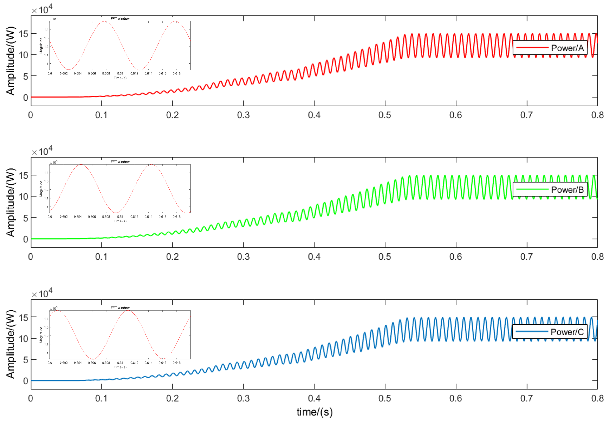
Figure 7 illustrates the output power of the T-type three-level inverter during normal operation. Due to the periodic averaging method, the output power undergoes a transition before entering a new steady-state process.
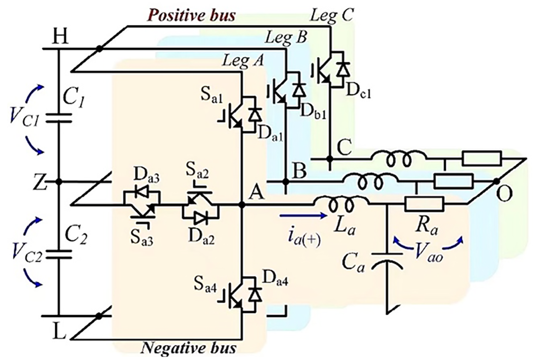
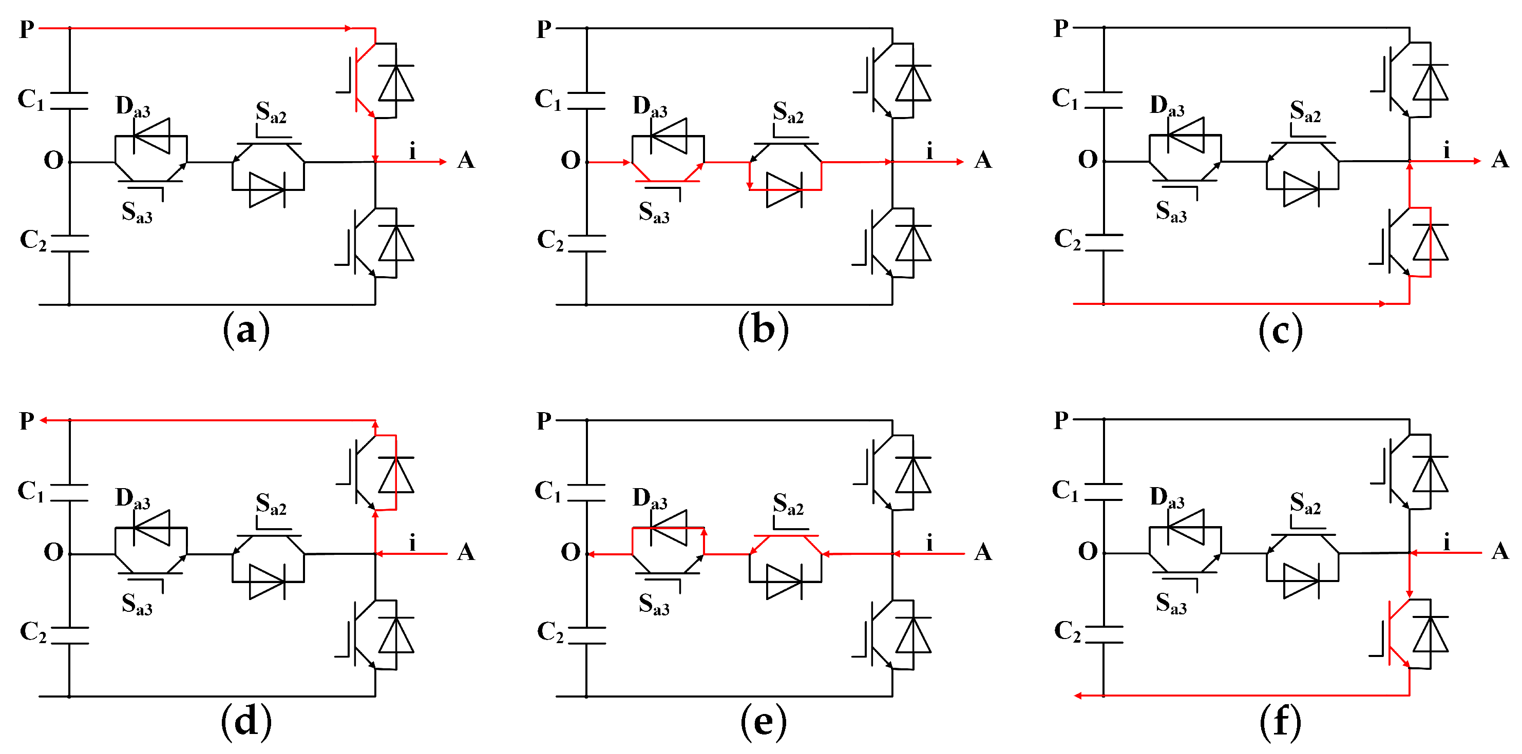
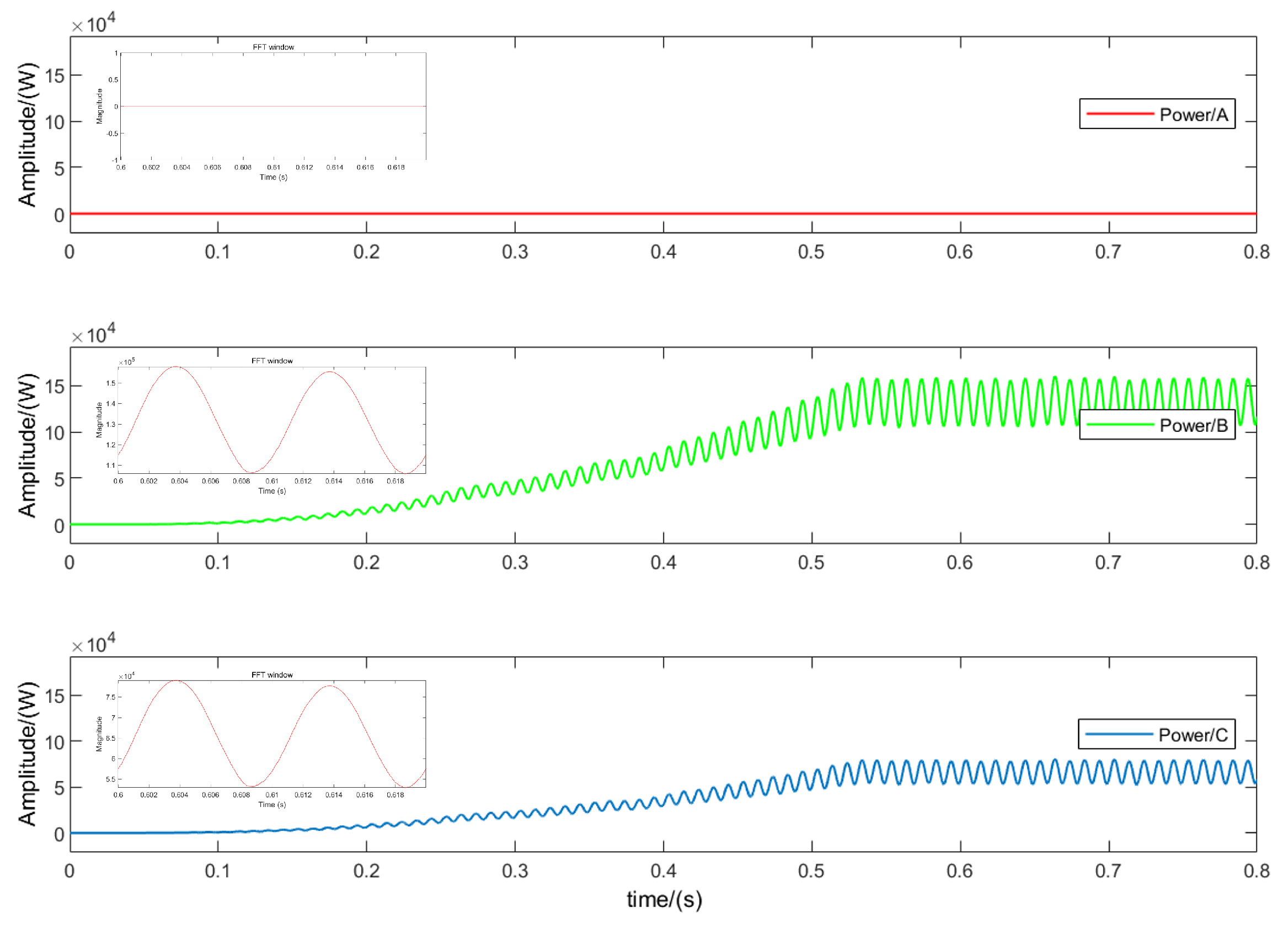
Figure 8 shows the simulation results of the OC fault of
in phase
A. When the output power enters a new steady-state process, it can be seen that compared with the normal state, after the OC fault of
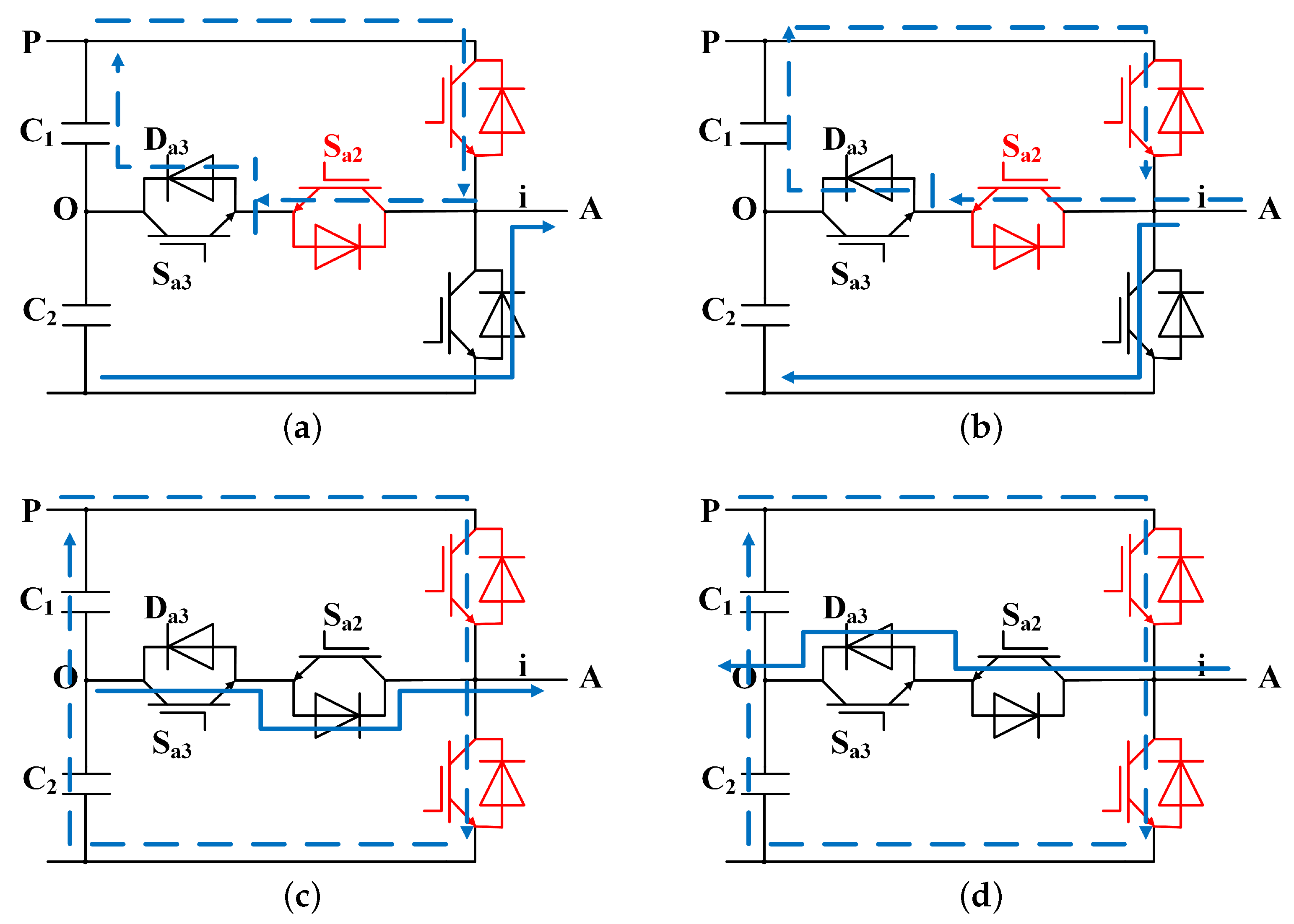
occurs, the output power is 0, and at the same time, other phases are accompanied by harmonics. This is because normally, the
A phase works in the
P state; the forward current flows through the DC bus and is transmitted to the load through the bridge arm switch, and the bridge arm outputs a positive level. However, when an open-circuit fault occurs in
, the
A phase bridge arm output cannot Connected to the DC bus, and the forward current will freewheel through the midpoint switch
and the diode
. At this time, the
A phase cannot work in the
P state, and the
P state is replaced by the
O state.
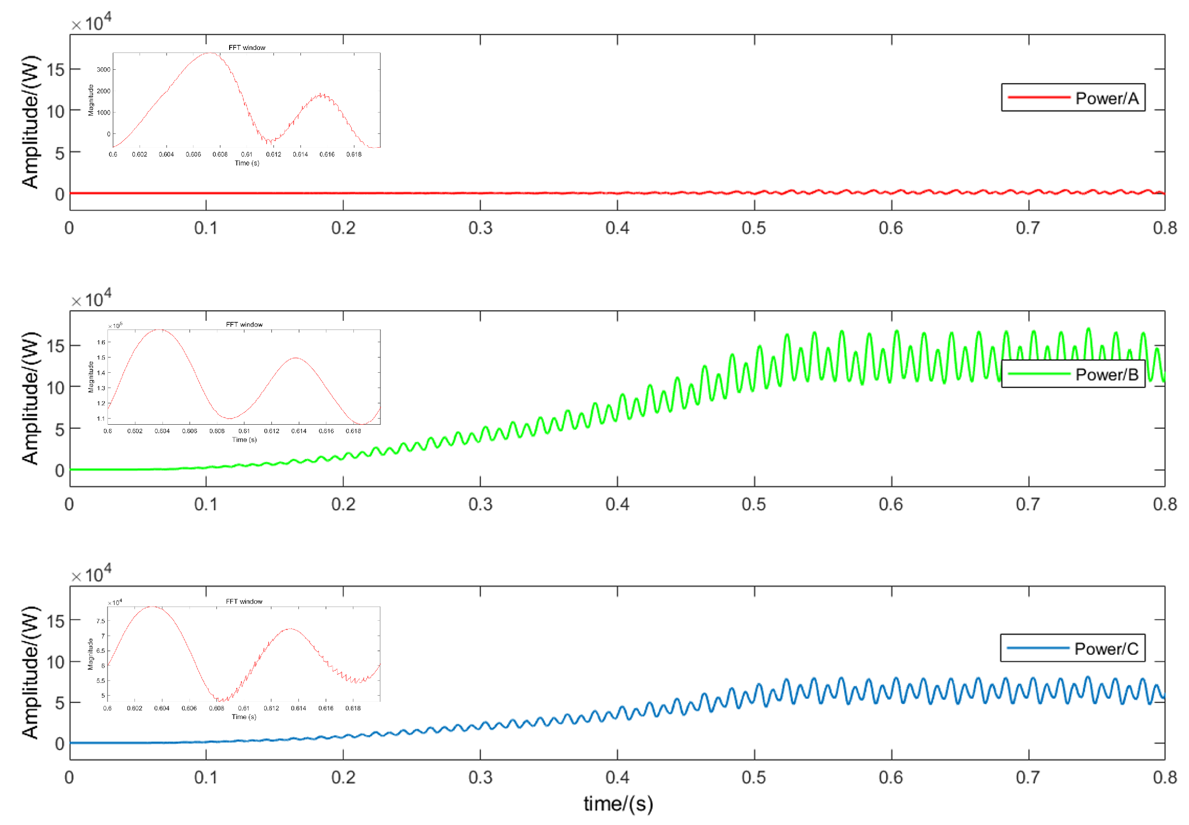
Figure 9 shows the simulation results of the OC fault of phase
A and
. Since the forward current can only continue to flow through the lower arm diode
after the fault, the operating state changes from
P to
N. It can be seen that when multiple IGBTs have OC faults at the same time, the power change is obviously different from the fault characteristics of a single IGBT OC fault. The simulation results are consistent with the theoretical analysis.
4.1. Dataset Selection
Since analyzing the power waveform and obtaining the fault characteristic signal in the time domain requires much calculation, the MATLAB library function FFT is used for the spectrum analysis of the three-phase output power waveform, and the amplitude and phase angle of each harmonic wave are obtained, with 50 as the base frequency. By integrating and combining simulation results, it is discovered that the component, fundamental harmonic, and second harmonic of the three-phase power signal contain most of the information about various faults. As a result, the component, fundamental amplitude , fundamental phase angle , second harmonic amplitude , and second harmonic phase angle are chosen as the input characteristic signals of the neural network.
4.1.1. Data Discretization Processing
The experimental part of this paper randomly selects 330 sets of fault-type data and divides the training set, validation set, and test set according to the ratio of 8:1:1. The final training set has 264 sets of fault-type data, and the validation set and test set contain 33 sets of fault-type data, respectively. Since the particle computation attribute reduction is based on discrete data, 30 sets of training sample data are randomly selected for discretization using the cluster discretization method in this paper. The decision table is obtained by further quantifying the discretized data and removing duplicate samples, as listed in
Table 4.
4.1.2. Data Reduction
In
Table 4,
U is the universe,
is the conditional attributes, and
is the decision attributes, respectively, represents the number of faulty devices.
Y is the identity matrix, which can be obtained from Equations (5)–(8):
However,
, i.e.,
, which means that decision
Table 4 is a compatible decision table.
First, by removing a single attribute, such as attribute
, we can obtain:
It indicates that the attribute depends on N and is irreducible.
Similarly, other attributes were removed one at a time to test whether the attribute and its related attribute set could represent complete information based on attribute dependency.
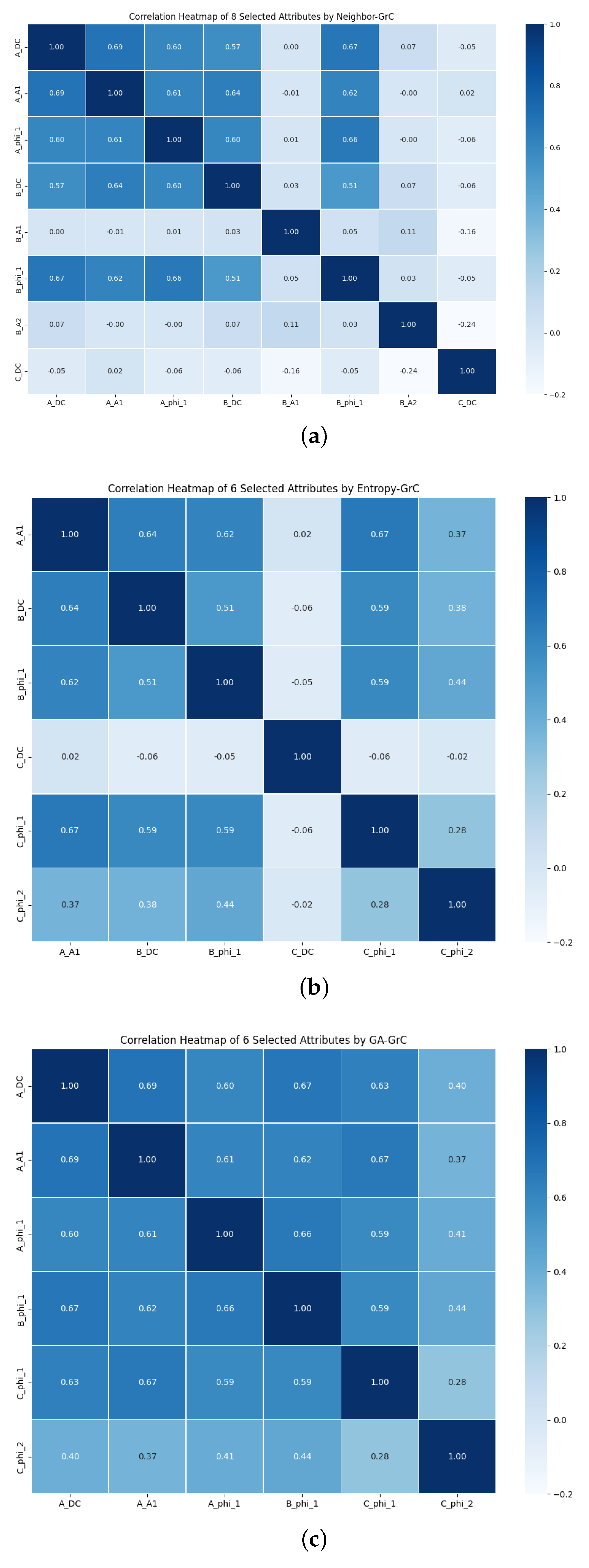
This article is grounded in the concept of binary granular representation of rough sets, utilizing mutual information attribute reduction algorithms based on Neighbor rough sets attribute reduction algorithm, entropy-based rough set attribute reduction algorithm, and a proposed genetic algorithm (GA)-based rough set attribute reduction algorithm. The comparative experiment of attribute reduction results is presented in
Table 5. Additionally,
Figure 10 illustrates the testing capabilities of the three algorithms in assessing the attribute reduction performance of rough sets under various discrimination conditions. It is evident that the GA algorithm significantly reduces the number of optimal attribute sets on this dataset compared to the other two algorithms, demonstrating the stronger attribute reduction ability of the GA-GrC algorithm.
4.2. Result Analysis
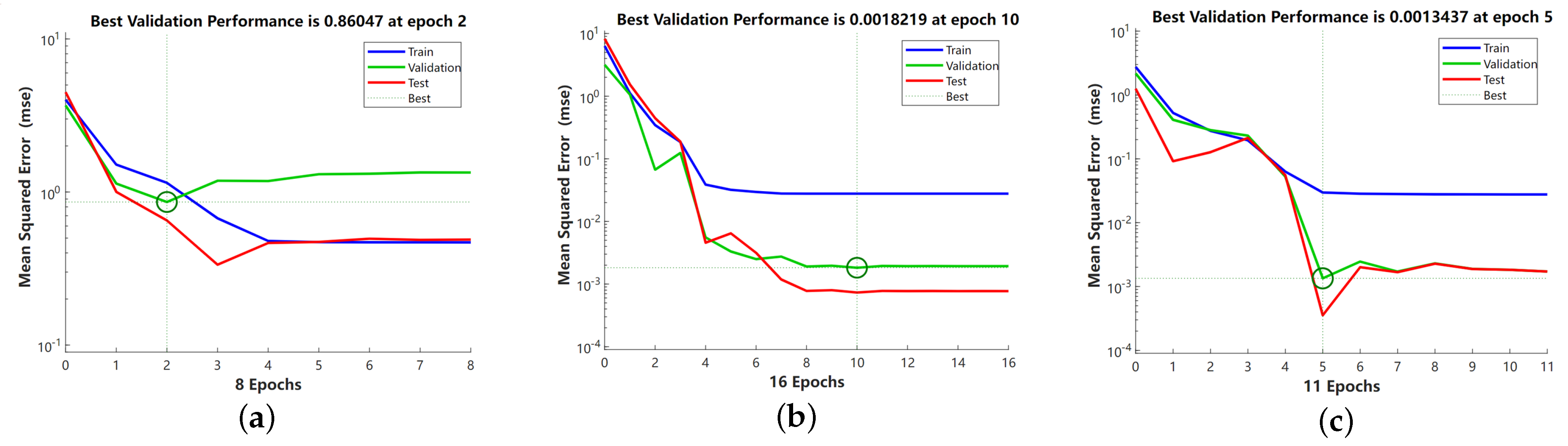
Figure 11 shows the training error curves of the binary grain matrix attribute approximation performance model for different optimization conditions on the training set, validation set, and test set, where the system automatically selects the stopping moment for the number of iterations in the adaptive condition. Where Train is the mean square error on the training set, Validation is the mean square error on the validation set, and Test is the mean square error on the test set. With the increase of epoch, the mean square error gradually stabilizes and oscillates in a small range, Although the ELM neural network based on Neighbor-GrC optimization converges quickly, the accuracy is far from the actual results. The ELM neural network based on Entropy-GrC optimization reaches the minimum convergence accuracy in the 10th iteration process. The ELM based on GA-GrC optimization proposed in this article has a minimum convergence after 5 iterations. Obviously, the GA-GrC-ELM neural network has a faster convergence speed and smaller convergence error because it introduces the crossover and mutation operators of GA during training, which expands the search space of the algorithm. The complementary advantages of genetic algorithm and binary granulation matrix knowledge reduction are improving the search ability and convergence speed, avoiding falling into local optimum, and improving the accuracy of the optimal solution.
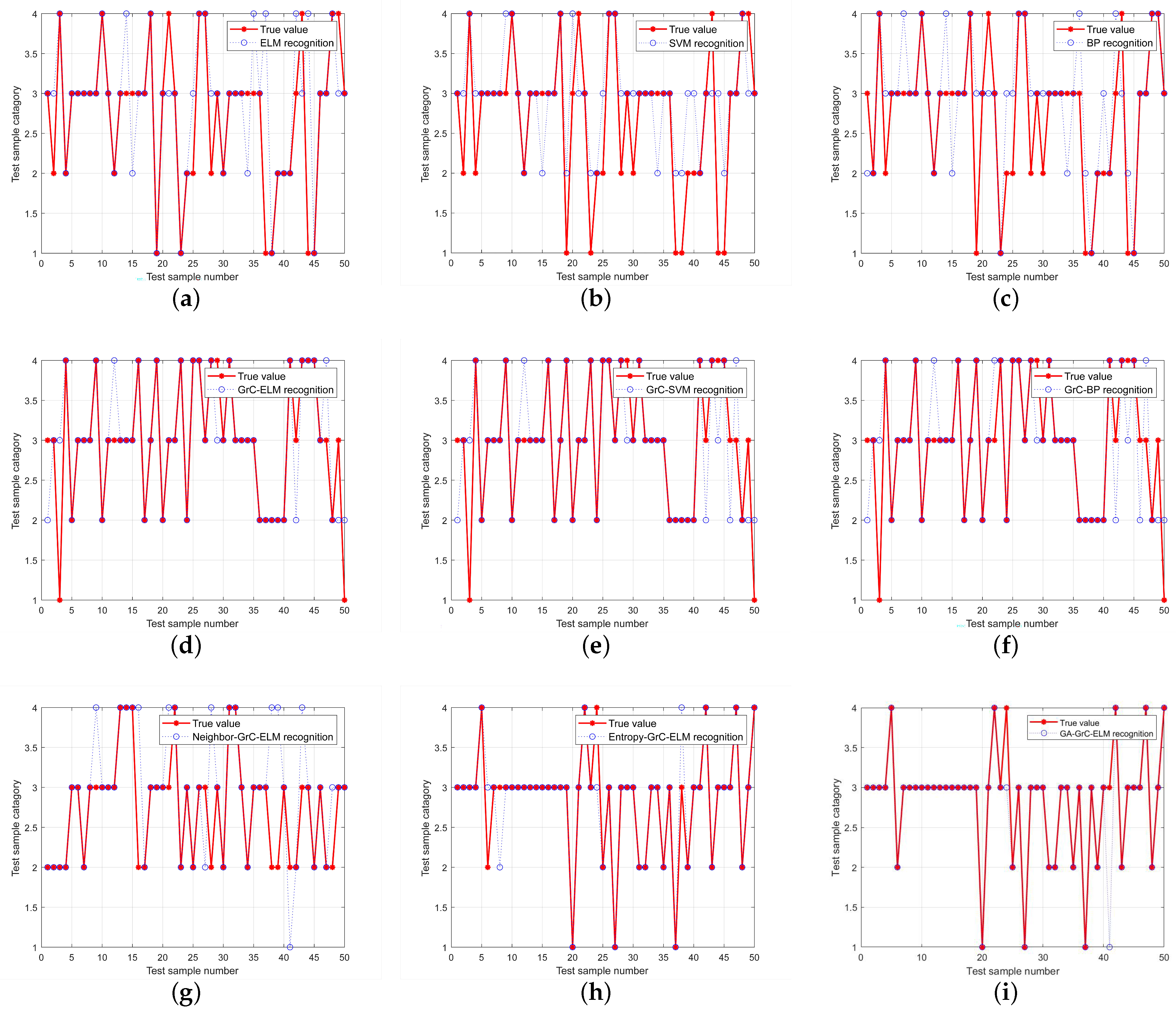
To verify the performance of the genetic algorithm-based binary grain matrix approximation proposed in this paper, the data sets before and after the reduction were used as the input data of the ELM network, respectively, and the network was trained with the maximum training times set to 1000, the learning rate set to 0.01, and the minimum error of the training target set to 0.01%. In
Figure 12,
Figure 12a–c are the fault-diagnosis results of the original dataset based on different neural networks. In comparison, since the input weights of ELM are random and fixed, there is no need for an iterative solution. It is necessary to solve the weights from the hidden layer to the output layer. Therefore, compared with the BP algorithm and SVM algorithm, the ELM neural network has a smaller training step within the specified range and a higher accuracy. After rough set reduction based on granular computing, as shown in
Figure 12d–f in the figure, the accuracy of each neural network has been significantly improved. It can be seen that the front-end processing of granular computing can effectively achieve data reduction, reducing redundant information and significantly improving the training accuracy of the neural network. Demonstrates the effectiveness of our proposed GrC algorithm.
Figure 12g–i show the classification performance of binary granulation matrices based on different optimization conditions. The results prove that the binary granulation matrix reduction method based on a genetic algorithm expands the search space and avoids falling into local optimality. This paper proposes that the binary granulation matrix reduction performance based on a genetic algorithm is the best.
Table 6 compares the performance of different algorithms in terms of accuracy, mean square error, and running time. In terms of accuracy, the GA-GrC-ELM algorithm proposed in this paper achieves 98%, which is significantly better than BP, SVM, and ELM algorithms. Although the accuracy of other algorithms also improved after the addition of GrC, it was still inferior to the algorithm in this paper. In addition, the algorithm in this paper also performs well in terms of mean square error and running time. Considered together, the GA-GrC-ELM-based algorithm can diagnose the T-type three-level inverter faults faster and more effectively.
In summary, the T-type three-level inverter fault-diagnosis method based on GA-GrC-ELM proposed in this paper fully utilizes the ability of granular computing theory to remove redundant information and combines the genetic algorithm to automatically calculate the fault diagnosis based on the fitness value of the population. It adapts to changing the probability values of crossover and mutation, effectively enhances its global search capability, and effectively solves the problem of diagnostic accuracy caused by the complex training samples and high dimensions of neural networks.


