
Deep Learning-Based Technique for Remote Sensing Image Enhancement Using Multiscale Feature Fusion


Abstract
:1. Introduction
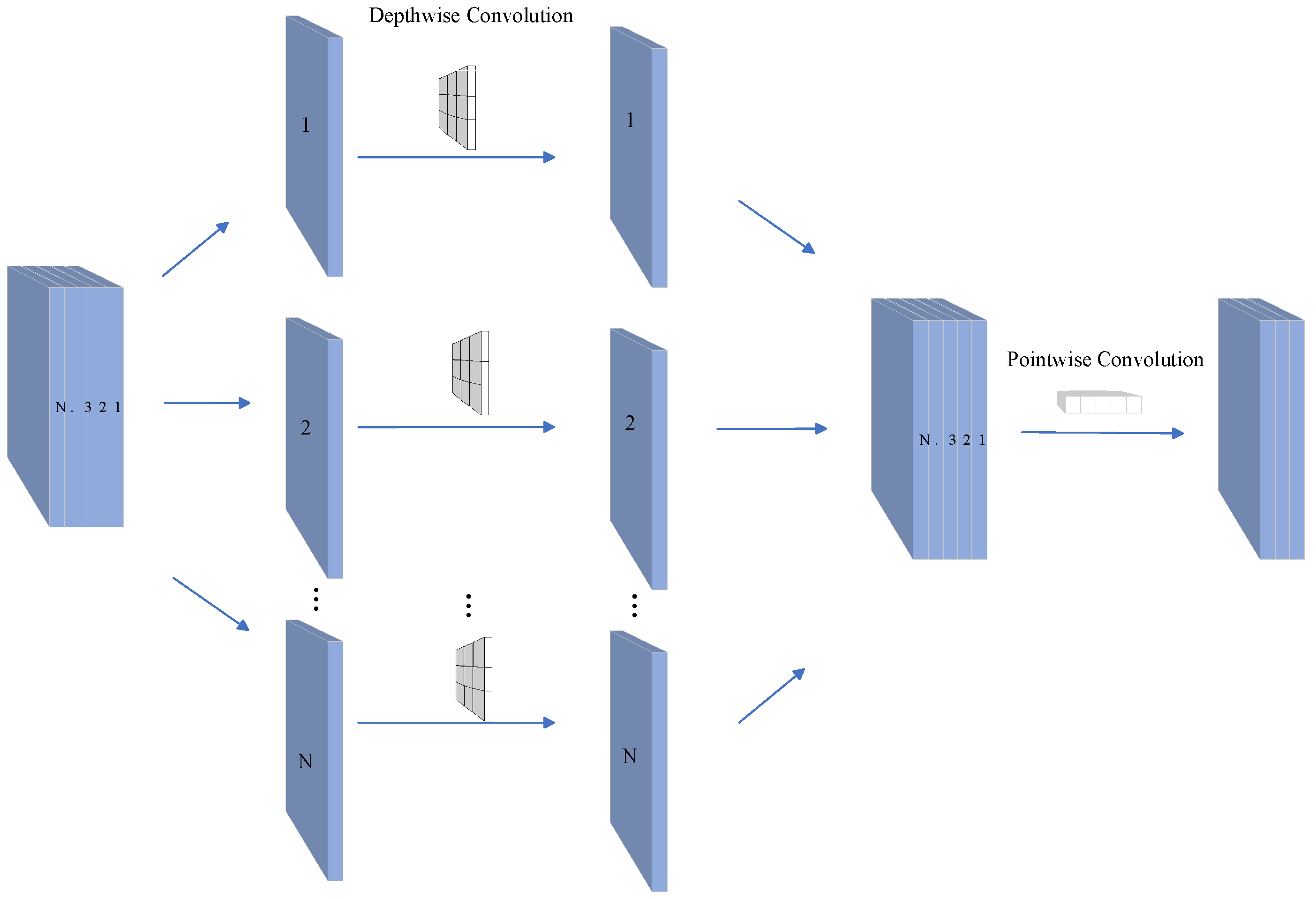
- Depthwise separable convolution is a lightweight convolution operation that significantly reduces the number of parameters and computations. Herein, we propose replacing the ordinary convolution in GSA-Net with depthwise separable convolution, reducing the number of parameters from 29.86 M to 7.06 M (a reduction of about 76%).
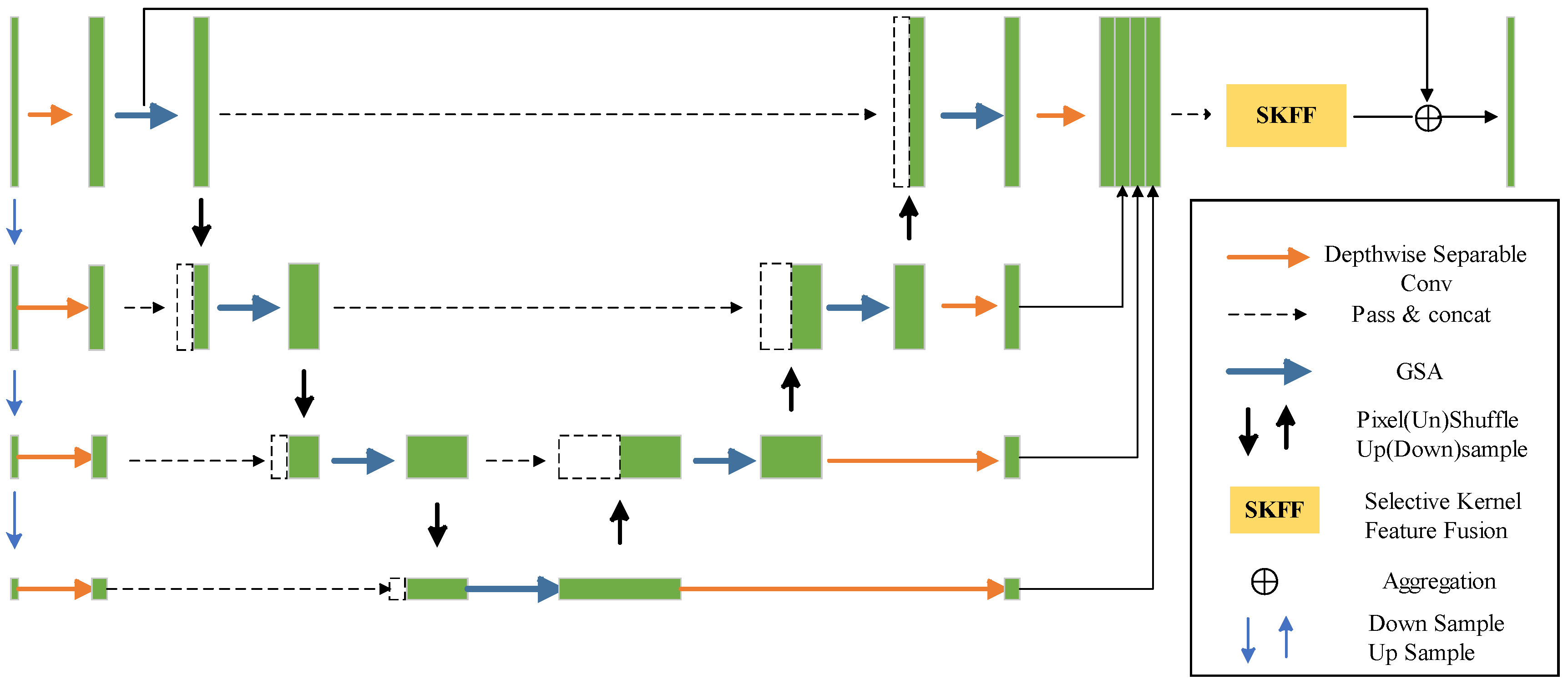
- A global attention module is introduced to weaken the noise response and integrate local information. Specifically, the global attention mechanism replaces the convolution layers of U-Net and is embedded into the network backbone.
- We propose an improved loss function that combines the peak signal-to-noise ratio (PSNR) and structural similarity (SSIM) quotient to avoid the model optimization direction deviation and gradient diffusion. This loss function guides the network to train and improve the convergence of the model.
- The proposed model is evaluated based on a synthesized low-light image enhancement dataset, and the results demonstrate that it achieves state-of-the-art performance in image enhancement. Moreover, we facilitate object detection on the enhanced images, which has positive implications for remote sensing images.
2. Related Studies
2.1. Data Augmentation
2.2. U-Net
3. Proposed Method
3.1. GSA-Net
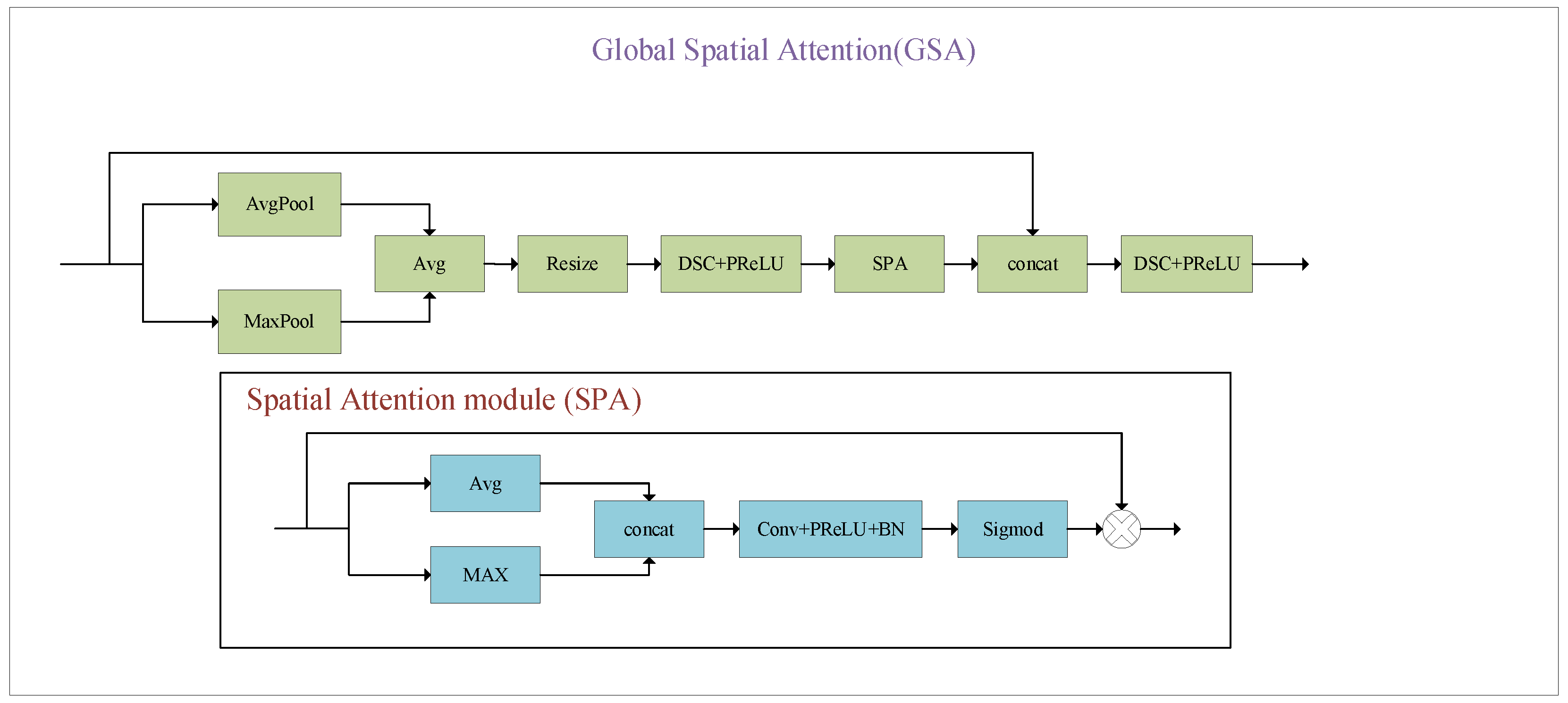
3.2. GSA Block
3.3. DSC
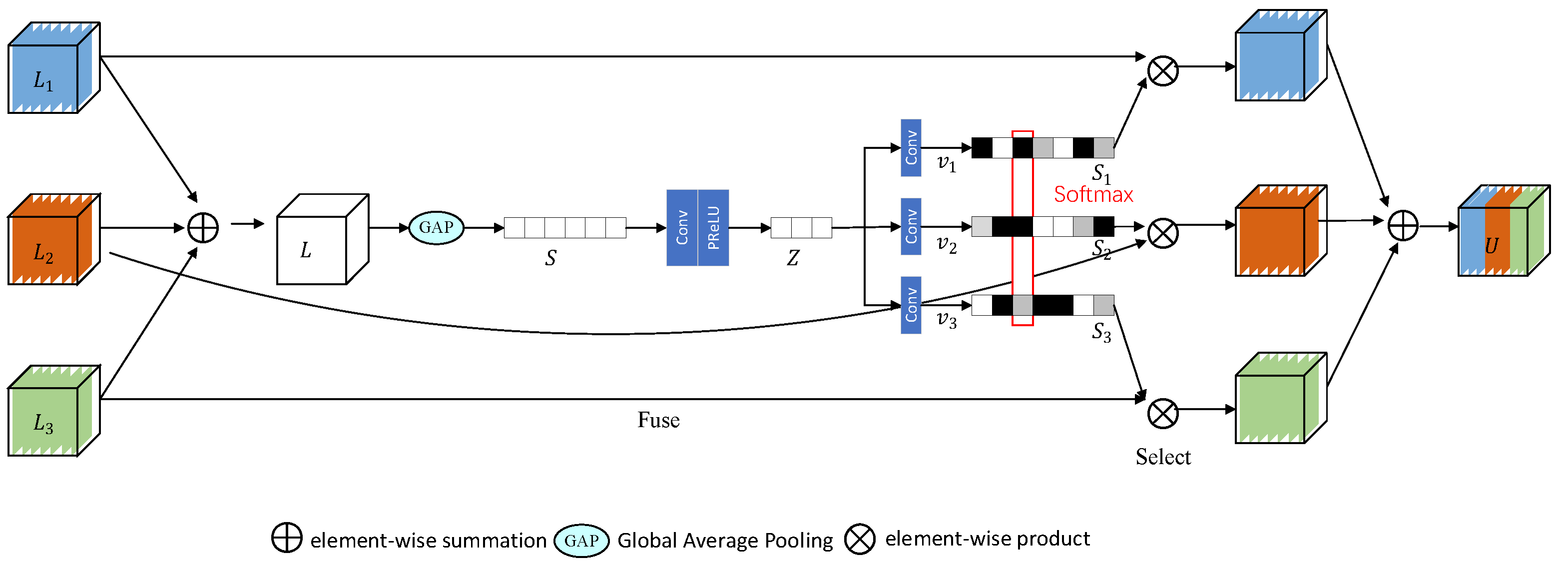
3.4. SKFF Module
3.5. Loss Function
4. Experiments
4.1. Experimental Design
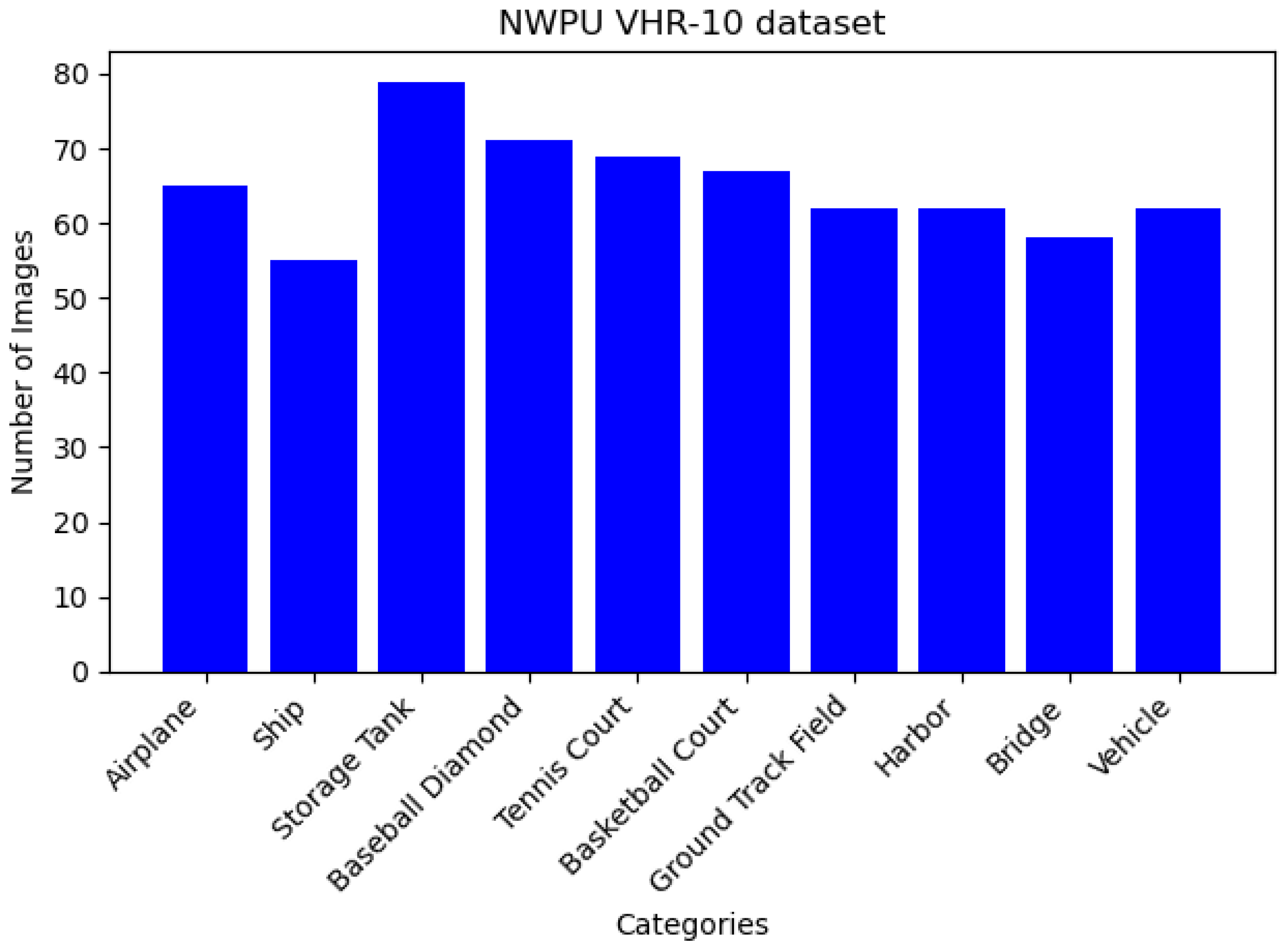
4.2. Dataset
4.3. Evaluation Metrics
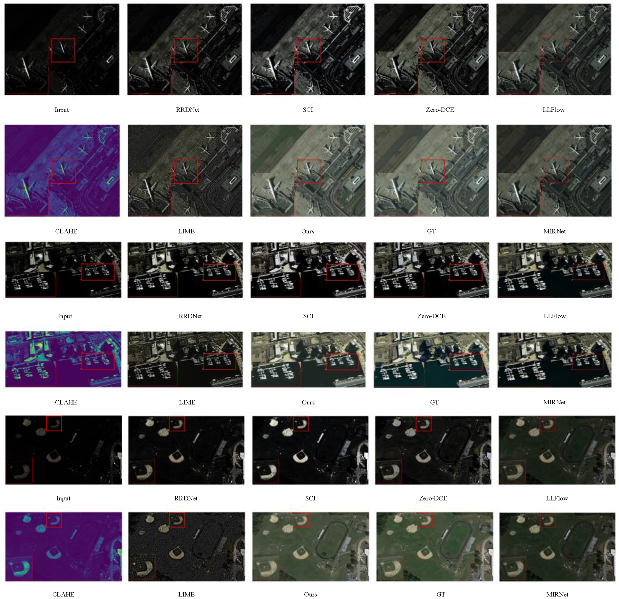
4.4. Qualitative Analysis of Experimental Results
4.5. Quantitative Analysis of Experimental Results
4.6. Loss Experiment
4.7. Ablation Experiment
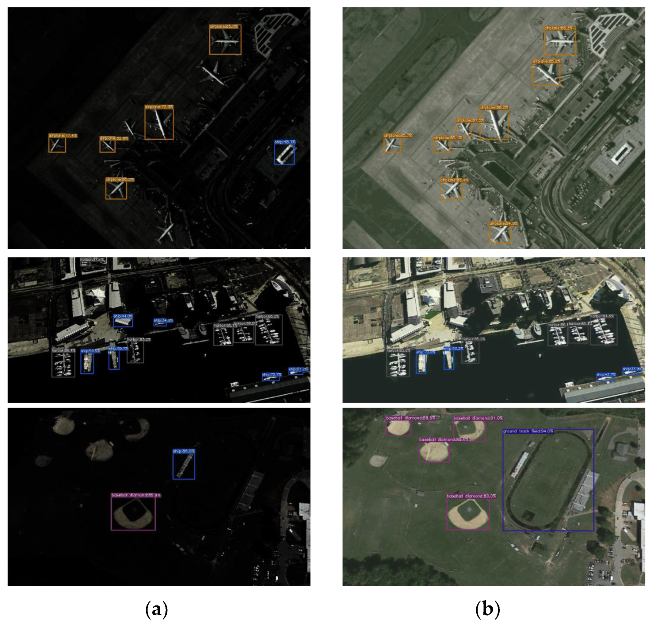
4.8. Case Study
5. Conclusions
Author Contributions
Funding
Institutional Review Board Statement
Informed Consent Statement
Data Availability Statement
Conflicts of Interest
References
- Demirel, H.; Ozcinar, C.; Anbarjafari, G. Satellite image contrast enhancement using discrete wavelet transform and singular value decomposition. IEEE Geosci. Remote Sens. Lett. 2010, 7, 333–337. [Google Scholar] [CrossRef]
- Gonzalez, R.C.; Woods, R.E. Digital Image Processing, 3rd ed.; Prentice-Hall: Upper Saddle River, NJ, USA, 2006. [Google Scholar]
- Ibrahim, H.; Kong, N.S.P. Brightness preserving dynamic histogram equalization for image contrast enhancement. IEEE Trans. Consum. Electron. 2007, 53, 1752–1758. [Google Scholar] [CrossRef]
- Arici, T.; Dikbas, S.; Altunbasak, Y. A histogram modification frame work and its application for image contrast enhancement. IEEE Trans. Image Process. 2009, 18, 1921–1935. [Google Scholar] [CrossRef] [PubMed]
- Huang, S.C.; Cheng, F.C.; Chiu, Y.S. Efficient contrast enhancement using adaptive gamma correction with weighting distribution. IEEE Trans. Image Process. 2013, 22, 1032–1041. [Google Scholar] [CrossRef] [PubMed]
- Celik, T. Two-dimensional histogram equalization and contrast enhancement. Pattern Recog. 2012, 45, 3810–3824. [Google Scholar] [CrossRef]
- Celik, T.; Tjahjadi, T. Contextual and variational contrast enhancement. IEEE Trans. Image Process. 2011, 20, 3431–3441. [Google Scholar] [CrossRef] [PubMed]
- Celik, T. Spatial entropy-based global and local image contrast enhancement. IEEE Trans. Image Process. 2014, 23, 5298–5308. [Google Scholar] [CrossRef]
- Demirel, H.; Anbarjafari, G.; Jahromi, M.N.S. Image equalization based on singular value decomposition. In Proceedings of the 2008 23rd International Symposium on Computer and Information Sciences, Istanbul, Turkey, 27–29 October 2008; pp. 1–5. [Google Scholar]
- Lee, E.; Kim, S.; Kang, W.; Seo, D.; Paik, J. Contrast enhancement using dominant brightness level analysis and adaptive intensity transformation for remote sensing images. IEEE Geosci. Remote Sens. Lett. 2013, 10, 62–66. [Google Scholar] [CrossRef]
- Jang, J.H.; Kim, S.D.; Ra, J.B. Enhancement of optical remote sensing images by subband-decomposed multiscale retinex with hybrid intensity transfer function. IEEE Geosci. Remote Sens. Lett. 2011, 8, 983–987. [Google Scholar] [CrossRef]
- Zhang, G.; Chen, Q.; Sun, Q. Illumination normalization among multiple remote-sensing images. IEEE Geosci. Remote Sens. Lett. 2014, 11, 1470–1474. [Google Scholar] [CrossRef]
- Lore, K.G.; Akintayo, A.; Sarkar, S. LLNet: A Deep Autoencoder Approach to Natural Low-light Image Enhancement. Pattern Recognit. 2017, 61, 650–662. [Google Scholar] [CrossRef]
- Shen, L.; Yue, Z.; Feng, F.; Chen, Q.; Liu, S.; Ma, J. Msr-Net: Low-light Image Enhancement Using Deep Convolutional Network. arXiv 2017, arXiv:1711.02488. Available online: https://arxiv.org/pdf/1711.02488.pdf (accessed on 1 December 2021).
- Wei, C.; Wang, W.; Yang, W.; Liu, J. Deep Retinex Decomposition for Low-light Enhancement. arXiv 2018, arXiv:1808.04560. Available online: https://arxiv.org/abs/1808.04560 (accessed on 1 December 2021).
- Han, H.; Chung, S.-W.; Kang, H.-G. Mirnet: Learning multiple identities representations in overlapped speech. arXiv 2020, arXiv:2008.01698. [Google Scholar]
- Zhang, C.; Yan, Q.; Zhu, Y.; Li, X.; Sun, J.; Zhang, Y. Attention-based network for low-light image enhancement. In Proceedings of the 2020 IEEE International Conference on Multimedia and Expo (ICME), London, UK, 6–10 July 2020; Volume 1. [Google Scholar]
- Ronneberger, O.; Fischer, P.; Brox, T. Unet: Convolutional networks for biomedical image segmentation. In Proceedings of the Medical Image Computing and Computer-Assisted Intervention–MICCAI 2015: 18th International Conference, Munich, Germany, 5–9 October 2015; Springer: Berlin/Heidelberg, Germany, 2015; Volume 1, pp. 234–241. [Google Scholar]
- Zamir, S.W.; Arora, A.; Khan, S.; Hayat, M.; Khan, F.S.; Yang, M.H.; Shao, L. Learning enriched features for real image restoration and enhancement. In Proceedings of the Computer Vision–ECCV 2020: 16th European Conference, Glasgow, UK, 23–28 August 2020; Springer: Berlin/Heidelberg, Germany, 2020; pp. 492–511. [Google Scholar]
- Long, J.; Shelhamer, E.; Darrell, T. Fully convolutional networks for semantic segmentation. In Proceedings of the IEEE Conference on Computer Vision and Pattern Recognition, Boston, MA, USA, 7–12 June 2015; pp. 3431–3440. [Google Scholar]
- Lin, T.Y.; Dollár, P.; Girshick, R.; He, K.; Hariharan, B.; Belongie, S. Feature pyramid networks for object detection. In Proceedings of the IEEE Conference on Computer Vision and Pattern Recognition, Honolulu, HI, USA, 21–26 July 2017; pp. 2117–2125. [Google Scholar]
- Li, Y.; Chen, X.; Zhu, Z.; Xie, L.; Huang, G.; Du, D.; Wang, X. Attention-guided unified network for panoptic segmentation. In Proceedings of the IEEE/CVF Conference on Computer Vision and Pattern Recognition, Long Beach, CA, USA, 15–20 June 2019; pp. 7026–7035. [Google Scholar]
- He, K.; Zhang, X.; Ren, S.; Sun, J. Deep residual learning for image recognition. In Proceedings of the IEEE Conference on Computer Vision and Pattern Recognition, Las Vegas, NV, USA, 27–30 June 2016; pp. 770–778. [Google Scholar]
- Zhang, Y.; Li, K.; Li, K.; Wang, L.; Zhong, B.; Fu, Y. Image super-resolution using very deep residual channel attention networks. In Proceedings of the European Conference on Computer Vision (ECCV), Munich, Germany, 8–14 September 2018; pp. 286–301. [Google Scholar]
- Sifre, L.; Mallat, S. Rigid-motion scattering for texture classification. arXiv 2014, arXiv:1403.1687. [Google Scholar]
- Chollet, F. Xception: Deep learning with depthwise separable convolutions. In Proceedings of the 2017 IEEE Conference on Computer Vision and Pattern Recognition (CVPR), Honolulu, HI, USA, 21–26 July 2017; pp. 1800–1807. [Google Scholar] [CrossRef]
- Iandola, F.N.; Han, S.; Moskewicz, M.W.; Ashraf, K.; Dally, W.J.; Keutzer, K. SqueezeNet: AlexNet-level accuracy with 50× fewer parameters and <0.5 MB model size. arXiv 2016, arXiv:1602.07360. [Google Scholar]
- Cai, J.; Gu, S.; Zhang, L. Learning a Deep Single Image Contrast Enhancer from Multi-exposure Images. IEEE Trans. Image Process. 2018, 27, 2049–2062. [Google Scholar] [CrossRef]
- Zhao, H.; Gallo, O.; Frosio, I.; Kautz, J. Loss Functions for Image Restoration with Neural Networks. IEEE Trans. Comput. Imaging 2016, 3, 47–57. [Google Scholar] [CrossRef]
- Fan, C.M.; Liu, T.J.; Liu, K.H. Compound Multi-branch Feature Fusion for Real Image Restoration. arXiv 2022, arXiv:2206.02748. Available online: https://arxiv.org/abs/2206.02748 (accessed on 7 August 2022).
- Studholme, C.; Hill, D.L.G.; Hawkes, D.J. An Overlap Invariant Entropy Measure of 3D Medical Image Alignment. Pattern Recognit. 1999, 32, 71–86. [Google Scholar] [CrossRef]
- Zhang, R.; Isola, P.; Efros, A.A.; Shechtman, E.; Wang, O. The unreasonable effectiveness of deep features as a perceptual metric. In Proceedings of the 2018 IEEE/CVF Conference on Computer Vision and Pattern Recognition, Salt Lake City, UT, USA, 18–23 June 2018; IEEE: Piscataway, NJ, USA, 2018; pp. 586–595. [Google Scholar]
- Hyndman, R.J.; Koehler, A.B. Another Look at Measures of Forecast Accuracy. Int. J. Forecast. 2006, 22, 679–688. [Google Scholar] [CrossRef]
- Guo, X.; Li, Y.; Ling, H. LIME: Low-light image enhancement via illumination map estimation. IEEE Trans. Image Process. 2016, 26, 982–993. [Google Scholar] [CrossRef] [PubMed]
- Yadav, G.; Maheshwari, S.; Agarwal, A. Contrast limited adaptive histogram equalization based enhancement for real time video system. In Proceedings of the 2014 International Conference on Advances in Computing, Communications and Informatics (ICACCI), Delhi, India, 24–27 September 2014; IEEE: Piscataway, NJ, USA, 2014; pp. 2392–2397. [Google Scholar]
- Ma, L.; Ma, T.; Liu, R.; Fan, X.; Luo, Z. Toward fast, flexible, and robust low-light image enhancement. In Proceedings of the IEEE/CVF Conference on Computer Vision and Pattern Recognition, New Orleans, LA, USA, 18–24 June 2022; pp. 5637–5646. [Google Scholar]
- Zhu, A.; Zhang, L.; Shen, Y.; Ma, Y.; Zhao, S.; Zhou, Y. Zero-shot restoration of underexposed images via robust retinex decomposition. In Proceedings of the 2020 IEEE International Conference on Multimedia and Expo (ICME), London, UK, 6–10 July 2020; IEEE: Piscataway, NJ, USA, 2020; pp. 1–6. [Google Scholar]
- Guo, C.; Li, C.; Guo, J.; Loy, C.C.; Hou, J.; Kwong, S.; Cong, R. Zero-reference deep curve estimation for low-light image enhancement. In Proceedings of the IEEE/CVF Conference on Computer Vision and Pattern Recognition, Seattle, WA, USA, 13–19 June 2020; pp. 1780–1789. [Google Scholar]
- Lai, W.S.; Huang, J.B.; Ahuja, N.; Yang, M.H. Fast and Accurate Image Super-resolution with Deep Laplacian Pyramid Networks. IEEE Trans. Pattern Anal. Mach. Intell. 2019, 41, 2599–2613. [Google Scholar] [CrossRef] [PubMed]
- Cai, J.F.; Candès, E.J.; Shen, Z. A singular value thresholding algorithm for matrix completion. SIAM J. Optim. 2010, 20, 1956–1982. [Google Scholar] [CrossRef]
- Wang, Y.; Wan, R.; Yang, W.; Li, H.; Chau, L.P.; Kot, A. Low-light image enhancement with normalizing flow. In Proceedings of the AAAI Conference on Artificial Intelligence, Virtually, 22 February–1 March 2022; Volume 36, pp. 2604–2612. [Google Scholar]
- Ge, Z.; Liu, S.; Wang, F.; Li, Z.; Sun, J. Yolox: Exceeding yolo series in 2021. arXiv 2021, arXiv:2107.08430. [Google Scholar]


| Operating Environment | Detailed Configuration |
|---|---|
| System | ubuntu20.04 |
| Processor Model | Intel Xeon Platinum 8255C @ 2.50 GHz |
| Graphics Card | RTX 2080 Ti(11 GB) |
| CUDA Version | 10.1 |
| Deep Learning Framework | Pytorch 1.11.0 |
| Parameter Combination | ||
|---|---|---|
| 1 | 0.85 | 2.0 |
| 2 | 0.90 | 3.5 |
| 3 | 0.80 | 1.8 |
| 4 | 0.88 | 4.0 |
| 5 | 0.82 | 2.8 |
| 6 | 0.95 | 1.3 |
| 7 | 0.86 | 3.2 |
| Evaluation Metrics | Algorithm | |||||||
|---|---|---|---|---|---|---|---|---|
| RRDNet | SCI | ZeroDCE | LLFlow | MIRNet | CLAHE | LIME | OURS | |
| PSNR | 19.378 | 21.356 | 20.784 | 23.516 | 24.339 | 15.632 | 17.413 | 30.110 |
| SSIM | 0.542 | 0.526 | 0.612 | 0.786 | 0.795 | 0.356 | 0.456 | 0.863 |
| LPIPS | 0.387 | 0.362 | 0.354 | 0.322 | 0.284 | 0.639 | 0.543 | 0.172 |
| SNR | 18.653 | 18.292 | 19.661 | 20.121 | 20.864 | 14.334 | 15.314 | 24.361 |
| NMI | 0.712 | 0.815 | 0.732 | 0.696 | 0.735 | 0.432 | 0.654 | 0.833 |
| NRMSE | 0.276 | 0.258 | 0.268 | 0.263 | 0.254 | 0.563 | 0.388 | 0.232 |
| Evaluation Metrics | Function | ||||
|---|---|---|---|---|---|
| MSE | MAE | Charbonnier | SSIM | PSNR/SSIM | |
| PSNR | 27.376 | 26.195 | 29.552 | 26.224 | 30.110 |
| SSIM | 0.811 | 0.834 | 0.867 | 0.851 | 0.863 |
| LPIPS | 0.245 | 0.342 | 0.189 | 0.263 | 0.172 |
| SNR | 21.369 | 20.475 | 24.726 | 23.698 | 24.361 |
| NMI | 0.791 | 0.735 | 0.812 | 0.789 | 0.833 |
| NRMSE | 0.312 | 0.368 | 0.225 | 0.267 | 0.232 |
| DSC | SKFF | GSA | PSNR | SSIM | Parameters |
|---|---|---|---|---|---|
| × | × | × | 20.287 | 0.542 | 30.37 M |
| √ | × | × | 18.689 | 0.533 | 6.88 M |
| × | √ | × | 25.645 | 0.758 | 30.07 M |
| × | × | √ | 23.332 | 0.637 | 30.16 M |
| × | √ | √ | 30.230 | 0.876 | 29.86 M |
| √ | √ | √ | 30.110 | 0.863 | 7.06 M |
Disclaimer/Publisher’s Note: The statements, opinions and data contained in all publications are solely those of the individual author(s) and contributor(s) and not of MDPI and/or the editor(s). MDPI and/or the editor(s) disclaim responsibility for any injury to people or property resulting from any ideas, methods, instructions or products referred to in the content. |
© 2024 by the authors. Licensee MDPI, Basel, Switzerland. This article is an open access article distributed under the terms and conditions of the Creative Commons Attribution (CC BY) license (https://creativecommons.org/licenses/by/4.0/).
Share and Cite
Zhao, M.; Yang, R.; Hu, M.; Liu, B. Deep Learning-Based Technique for Remote Sensing Image Enhancement Using Multiscale Feature Fusion. Sensors 2024, 24, 673. https://doi.org/10.3390/s24020673
Zhao M, Yang R, Hu M, Liu B. Deep Learning-Based Technique for Remote Sensing Image Enhancement Using Multiscale Feature Fusion. Sensors. 2024; 24(2):673. https://doi.org/10.3390/s24020673
Chicago/Turabian StyleZhao, Ming, Rui Yang, Min Hu, and Botao Liu. 2024. "Deep Learning-Based Technique for Remote Sensing Image Enhancement Using Multiscale Feature Fusion" Sensors 24, no. 2: 673. https://doi.org/10.3390/s24020673