
MFTR-Net: A Multi-Level Features Network with Targeted Regularization for Large-Scale Point Cloud Classification


Abstract
:1. Introduction
- (1)
- We propose a new feature construction method for large-scale point clouds, which can effectively calculate the multi-level local feature information of the point cloud from the irregular point cloud data.
- (2)
- We present the MFTR-Net framework for point cloud classification. The designed encoder–decoder model can effectively extract the local feature information of the point cloud from the input feature map, and strengthen the attention to spatial information.
- (3)
- We conduct extensive experiments on the 3D point cloud dataset, Oakland. The experimental results show that the proposed MFTR-Net has achieved satisfactory results in large-scale point cloud classification tasks.
2. Related Work
3. MFTR-Net: A Multi-Level Features Network with Targeted Regularization for Large-Scale Point Cloud Classification
3.1. Feature Construction for Point Clouds
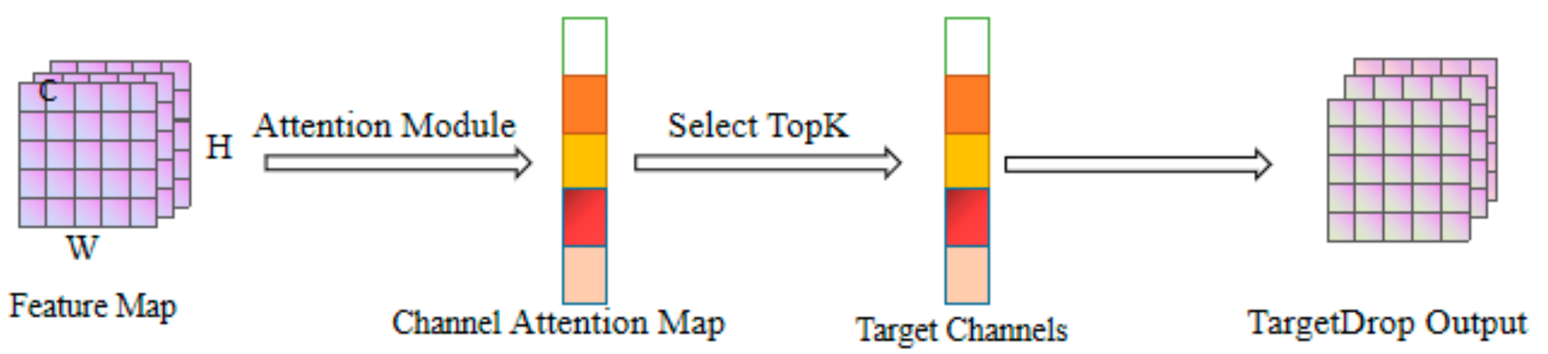
3.2. TargetDrop-Based MFTR-Net
3.3. MFTR-Net for Large-Scale Point Cloud Classification
4. Analysis of Experimental Results
5. Ablation Study
6. Conclusions
Author Contributions
Funding
Institutional Review Board Statement
Informed Consent Statement
Data Availability Statement
Conflicts of Interest
References
- Liu, R.; Zhang, G.; Wang, J.; Zhao, S. Cross-modal 360° depth completion and reconstruction for large-scale indoor environment. IEEE Trans. Intell. Transp. Syst. 2022, 23, 25180–25190. [Google Scholar] [CrossRef]
- Zhang, G.; Weng, H.; Liu, R.; Zhang, M.; Zhang, Z. Point Clouds Classification of Large Scenes based on Blueprint Separation Convolutional Neural Network. In Proceedings of the 2022 IEEE 25th International Conference on Computer Supported Cooperative Work in Design (CSCWD), Hangzhou, China, 4–6 May 2022; IEEE: Piscataway, NJ, USA, 2022. [Google Scholar]
- Sun, J.; Lai, Z. Using random forest to select and classify features of airborne LiDAR data in urban area. J. Wuhan Univ. 2014, 39, 1310–1313. [Google Scholar]
- Fang, J.; Zhou, D.; Zhao, J.; Tang, C.; Xu, C.Z.; Zhang, L. LiDAR-CS Dataset: LiDAR Point Cloud Dataset with Cross-Sensors for 3D Object Detection. arXiv 2023, arXiv:2301.12515. [Google Scholar]
- Guo, Y.; Wang, H.; Hu, Q.; Liu, H.; Liu, L.; Bennamoun, M. Deep learning for 3d point clouds: A survey. IEEE Trans. Pattern Anal. Mach. Intell. 2020, 43, 4338–4364. [Google Scholar] [CrossRef] [PubMed]
- Sarker, A.K.; Ahmad, F.Y.; Dwyer, M.B. PCV: A Point Cloud-Based Network Verifier. arXiv 2023, arXiv:2301.11806. [Google Scholar]
- Venkanna Sheshappanavar, S.; Kambhamettu, C. Local Neighborhood Features for 3D Classification. arXiv 2022, arXiv:2212.05140. [Google Scholar]
- Min, C.; Zhao, D.; Xiao, L.; Nie, Y.; Dai, B. Voxel-mae: Masked autoencoders for pre-training large-scale point clouds. arXiv 2022, arXiv:2206.09900. [Google Scholar]
- Zhu, T.; Guan, Y.; Li, A. PointManifoldCut: Point-wise Augmentation in the Manifold for Point Clouds. arXiv 2021, arXiv:2109.07324. [Google Scholar]
- Wen, C.; Long, J.; Yu, B.; Tao, D. PointWavelet: Learning in Spectral Domain for 3D Point Cloud Analysis. arXiv 2023, arXiv:2302.05201. [Google Scholar]
- Zhang, Z.; Hua, B.S.; Yeung, S.K. Riconv++: Effective rotation invariant convolutions for 3d point clouds deep learning. Int. J. Comput. Vis. 2022, 130, 1228–1243. [Google Scholar] [CrossRef]
- Zhang, Z.; Liu, R.; Xie, E.; Zhang, G. Large Scale Point Cloud Classification Base on Graph-MLP++. In Proceedings of the 2022 IEEE 9th International Conference on Data Science and Advanced Analytics (DSAA), Shenzhen, China, 13–16 October 2022; IEEE: Piscataway, NJ, USA, 2022. [Google Scholar]
- Li, Z.; Gao, P.; Yuan, H.; Wei, R. Dynamic Local Feature Aggregation for Learning on Point Clouds. arXiv 2023, arXiv:2301.02836. [Google Scholar]
- Chen, B.; Pang, Y.; Li, Z.; Lu, H.; Liang, X. Photon counting lidar point cloud filtering based on random forest. J. Geo-Inf. Sci. 2019, 21, 898–906. [Google Scholar]
- Melnyk, P.; Robinson, A.; Wadenbäck, M.; Felsberg, M. TetraSphere: A Neural Descriptor for O (3)-Invariant Point Cloud Classification. arXiv 2022, arXiv:2211.14456. [Google Scholar]
- Zhao, H.; Jiang, L.; Jia, J.; Torr, P.H.; Koltun, V. Point transformer. In Proceedings of the IEEE/CVF International Conference on Computer Vision, Montreal, BC, Canada, 11–17 October 2021; pp. 16259–16268. [Google Scholar]
- Wang, Z.; Arablouei, R.; Liu, J.; Borges, P.; Bishop-Hurley, G.; Heaney, N. Point-Syn2Real: Semi-Supervised Synthetic-to-Real Cross-Domain Learning for Object Classification in 3D Point Clouds. arXiv 2022, arXiv:2210.17009. [Google Scholar]
- Wen, C.; Li, X.; Yao, X.; Peng, L.; Chi, T. Airborne LiDAR point cloud classification with global-local graph attention convolution neural network. ISPRS J. Photogramm. Remote Sens. 2021, 173, 181–194. [Google Scholar] [CrossRef]
- Park, J.; Kim, C.; Kim, S.; Jo, K. PCSCNet: Fast 3D semantic segmentation of LiDAR point cloud for autonomous car using point convolution and sparse convolution network. Expert Syst. Appl. 2023, 212, 118815. [Google Scholar] [CrossRef]
- Yang, F.; Cao, Y.; Xue, Q.; Jin, S.; Li, X.; Zhang, W. Contrastive Embedding Distribution Refinement and Entropy-Aware Attention for 3D Point Cloud Classification. arXiv 2022, arXiv:2201.11388. [Google Scholar]
- Zhu, H.; Zhao, X. Targetdrop: A targeted regularization method for convolutional neural networks. In Proceedings of the ICASSP 2022—2022 IEEE International Conference on Acoustics, Speech and Signal Processing (ICASSP), Singapore, 22–27 May 2022; IEEE: Piscataway, NJ, USA, 2022; pp. 3283–3287. [Google Scholar]
- Hu, Y.; You, H.; Wang, Z.; Wang, Z.; Zhou, E.; Gao, Y. Graph-MLP: Node classification without message passing in graph. arXiv 2021, arXiv:2106.04051. [Google Scholar]
- Munoz, D.; Bagnell, J.A.; Vandapel, N.; Hebert, M. Contextual classification with functional max-margin markov networks. In Proceedings of the 2009 IEEE Conference on Computer Vision and Pattern Recognition, Miami, FL, USA, 20–25 June 2009; IEEE: Piscataway, NJ, USA, 2009; pp. 975–982. [Google Scholar]
- Oviedo-de la Fuente, M.; Cabo, C.; Ordóñez, C.; Roca-Pardiñas, J. A Distance Correlation Approach for Optimum Multiscale Selection in 3D Point Cloud Classification. Mathematics 2021, 9, 1328. [Google Scholar] [CrossRef]
- Chen-Chieh, F.; Zhou, G. Automating Parameter Learning for Classifying Terrestrial LiDAR Point Cloud Using 2D Land Cover Maps. Remote Sens. 2018, 10, 1192. [Google Scholar]
- Wang, L.; Meng, W.; Xi, R.; Zhang, Y.; Lu, L.; Zhang, X. Large-scale 3D point cloud classification based on feature description matrix by CNN. In Proceedings of the 31st International Conference on Computer Animation and Social Agents, Beijing, China, 21–23 May 2018; pp. 43–47. [Google Scholar]
- Wang, L.; Meng, W.; Xi, R.; Zhang, Y.; Ma, C.; Lu, L.; Zhang, X. 3D point cloud analysis and classification in large-scale scene based on deep learning. IEEE Access 2019, 7, 55649–55658. [Google Scholar] [CrossRef]
- Merkurjev, E. A Fast Graph-Based Data Classification Method with Applications to 3D Sensory Data in the Form of Point Clouds. Pattern Recognit. Lett. 2020, 136, 154–160. [Google Scholar] [CrossRef]
- Kumar, B.; Pandey, G.; Lohani, B.; Misra, S.C. A framework for automatic classification of mobile LiDAR data using multiple regions and 3D CNN architecture. Int. J. Remote Sens. 2020, 41, 5588–5608. [Google Scholar] [CrossRef]


| Type | Components |
|---|---|
| 3D eigenvalues | |
| 2D eigenvalues |
| Label | Training Dataset | Test Dataset |
|---|---|---|
| Vegetation | 14,441 | 9278 |
| Wire | 2571 | 481 |
| Pole | 1086 | 368 |
| Ground | 4713 | 71,863 |
| Facade | 14,121 | 7821 |
| Total | 36,932 | 89,811 |
| Pole | Vegetation | Wire | Ground | Facade | OA | |
|---|---|---|---|---|---|---|
| Cabo [24] | 77.3 | 80.6 | 80.4 | 99.2 | 92.9 | 86.1 |
| Chen-Chieh [25] | - | - | - | 100.0 | 94.7 | 97.0 |
| Wang [26] | 68.4 | 80.6 | 92.9 | 98.3 | 71.1 | 94.7 |
| Wang [27] | 70.1 | 80.5 | 93.0 | 98.2 | 70.9 | 94.6 |
| Ekaterina [28] | 28.7 | 97.4 | 12.5 | 98.2 | 90.8 | 91.6 |
| Kumar [29] | 70.9 | 94.7 | - | 97.9 | 94.4 | - |
| Our method | 21.5 | 93.8 | 20.1 | 99.5 | 98.1 | 98.0 |
| Warm-Up | Deep learning | Accuracy |
|---|---|---|
| √ | - | 89.5 |
| √ | √ | 98.3 |
| - | - | 88.1 |
| - | √ | 98.0 |
| Pole | Vegetation | Wire | Ground | Facade | OA | |
|---|---|---|---|---|---|---|
| 3D | 0.0 | 84.1 | 30.3 | 99.7 | 92.4 | 96.7 |
| 3D + 2Dx | 10.0 | 97.4 | 8.2 | 94.4 | 82.0 | 85.6 |
| 3D + 2Dy | 0.0 | 87.6 | 0.0 | 65.3 | 0.0 | 61.3 |
| 3D + 2Dz | 0.0 | 99.7 | 0.0 | 99.4 | 0.0 | 89.8 |
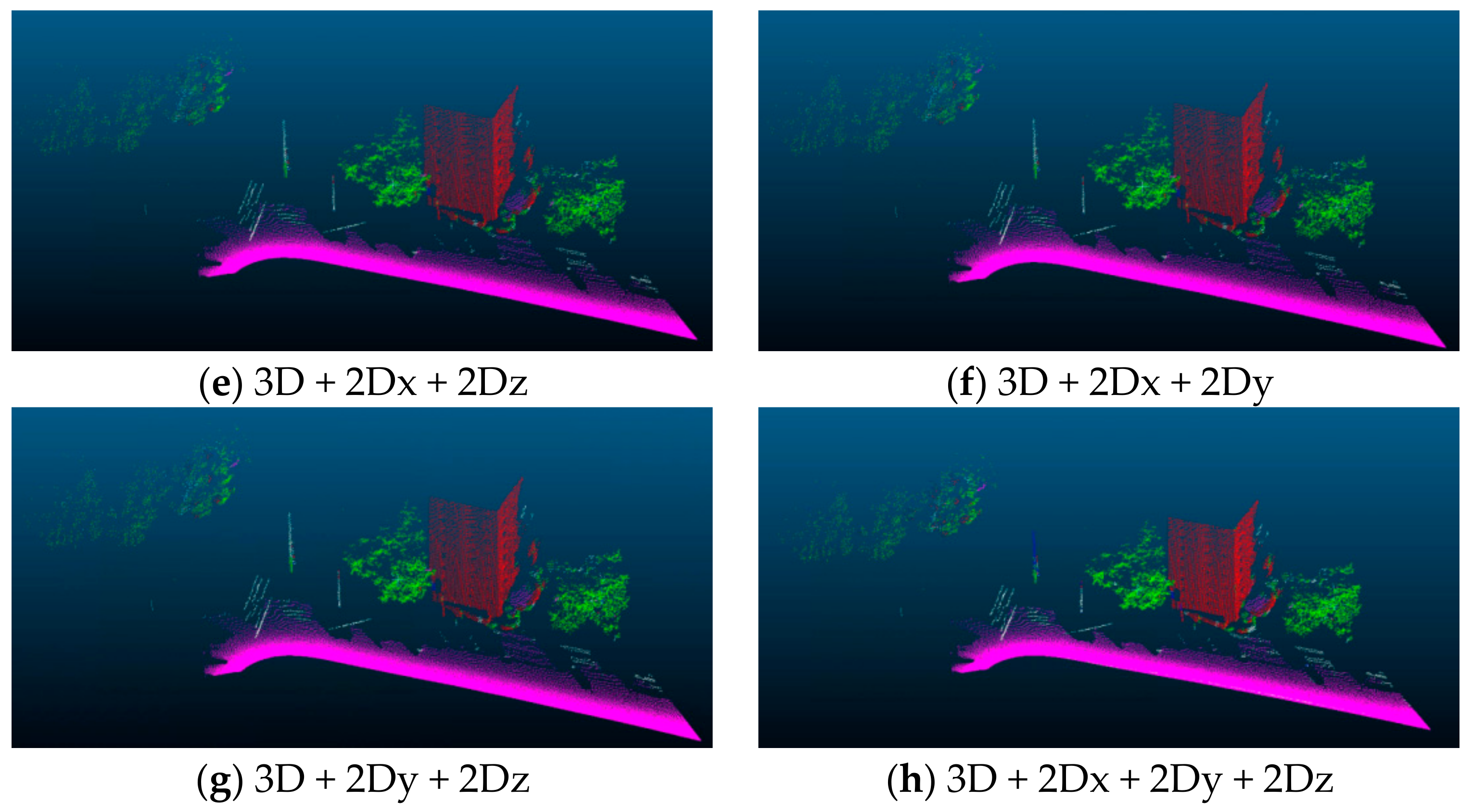
| 3D + 2Dx + 2Dz | 0.0 | 99.9 | 0.0 | 99.4 | 0.0 | 89.8 |
| 3D + 2Dx + 2Dy | 25.0 | 99.9 | 0.0 | 97.1 | 38.0 | 88.5 |
| 3D + 2Dy + 2Dz | 16.8 | 99.9 | 0.0 | 99.2 | 0.0 | 89.7 |
| 3D + 2Dx + 2Dy + 2Dz | 21.5 | 93.8 | 20.1 | 99.5 | 98.1 | 98.0 |
Disclaimer/Publisher’s Note: The statements, opinions and data contained in all publications are solely those of the individual author(s) and contributor(s) and not of MDPI and/or the editor(s). MDPI and/or the editor(s) disclaim responsibility for any injury to people or property resulting from any ideas, methods, instructions or products referred to in the content. |
© 2023 by the authors. Licensee MDPI, Basel, Switzerland. This article is an open access article distributed under the terms and conditions of the Creative Commons Attribution (CC BY) license (https://creativecommons.org/licenses/by/4.0/).
Share and Cite
Liu, R.; Zhang, Z.; Dai, L.; Zhang, G.; Sun, B. MFTR-Net: A Multi-Level Features Network with Targeted Regularization for Large-Scale Point Cloud Classification. Sensors 2023, 23, 3869. https://doi.org/10.3390/s23083869
Liu R, Zhang Z, Dai L, Zhang G, Sun B. MFTR-Net: A Multi-Level Features Network with Targeted Regularization for Large-Scale Point Cloud Classification. Sensors. 2023; 23(8):3869. https://doi.org/10.3390/s23083869
Chicago/Turabian StyleLiu, Ruyu, Zhiyong Zhang, Liting Dai, Guodao Zhang, and Bo Sun. 2023. "MFTR-Net: A Multi-Level Features Network with Targeted Regularization for Large-Scale Point Cloud Classification" Sensors 23, no. 8: 3869. https://doi.org/10.3390/s23083869