


Optimization of the Outlet Shape of an Air Circulation System for Reduction of Indoor Temperature Difference

Abstract
:1. Introduction
2. Theoretical Background
2.1. Design of Experiment
2.1.1. Taguchi Method
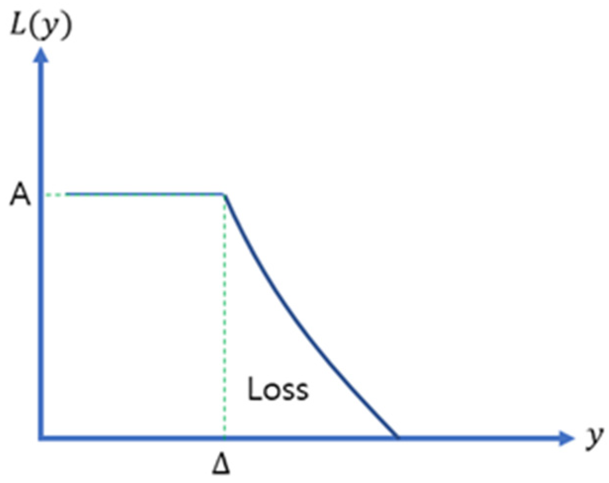
2.1.2. Loss Function
2.2. Analysis Model
2.2.1. Flow Field Governing Equation
- (1)
- Law of Conservation of Mass
- (2)
- Momentum Equation
2.2.2. Calculation of Turbulent Flow
- (1)
- Turbulence transport model
3. Analysis Model
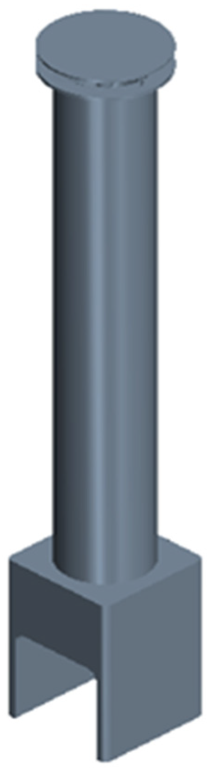
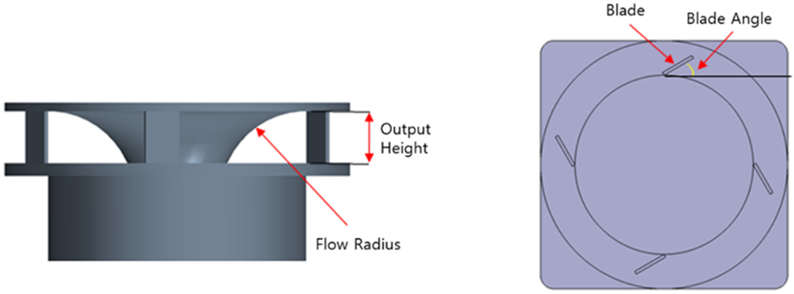
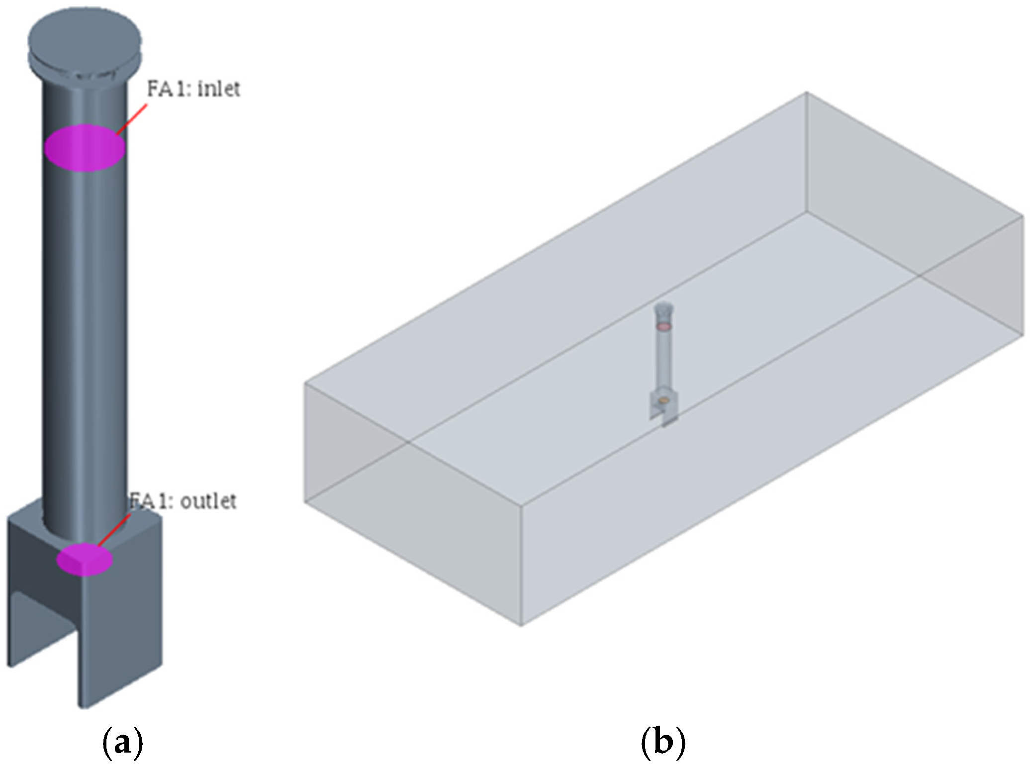
3.1. Shape Model
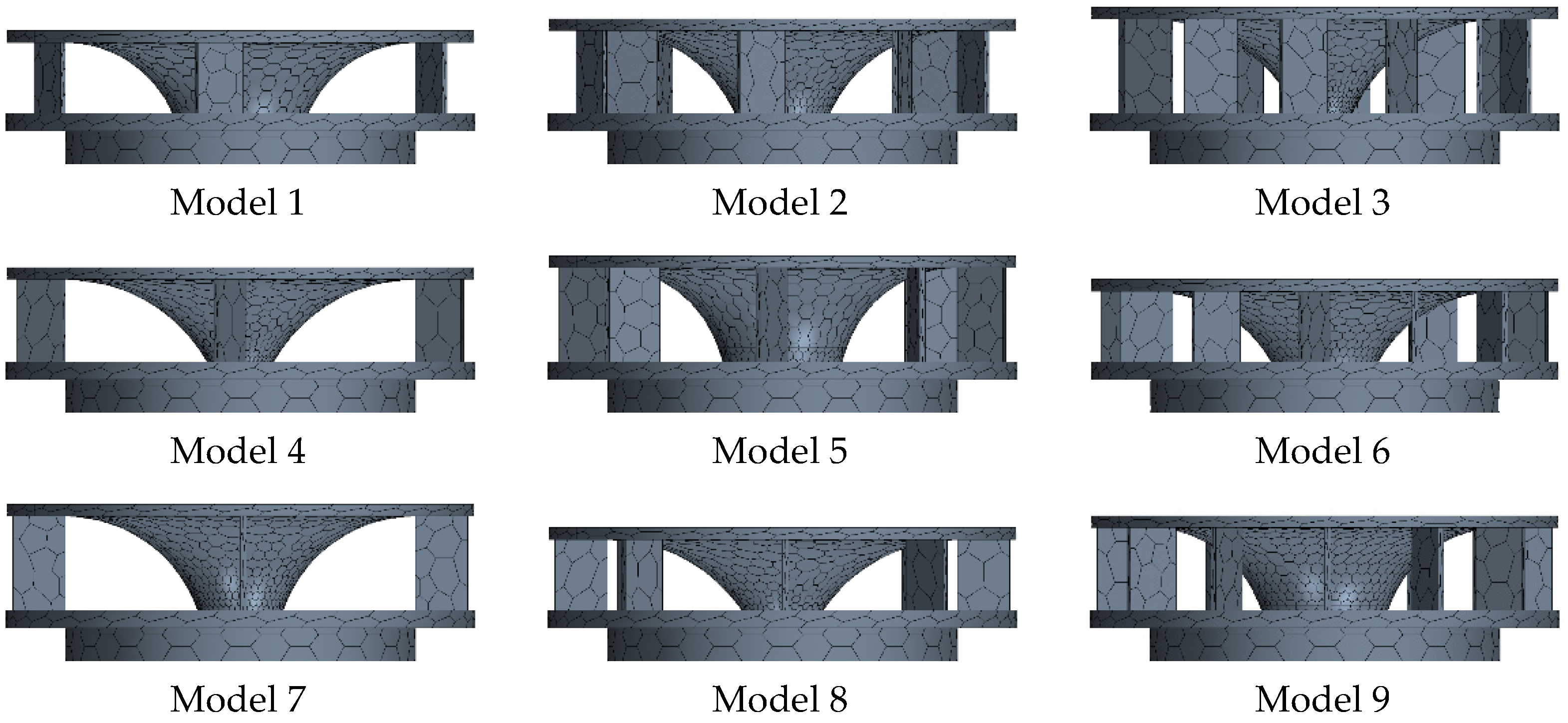
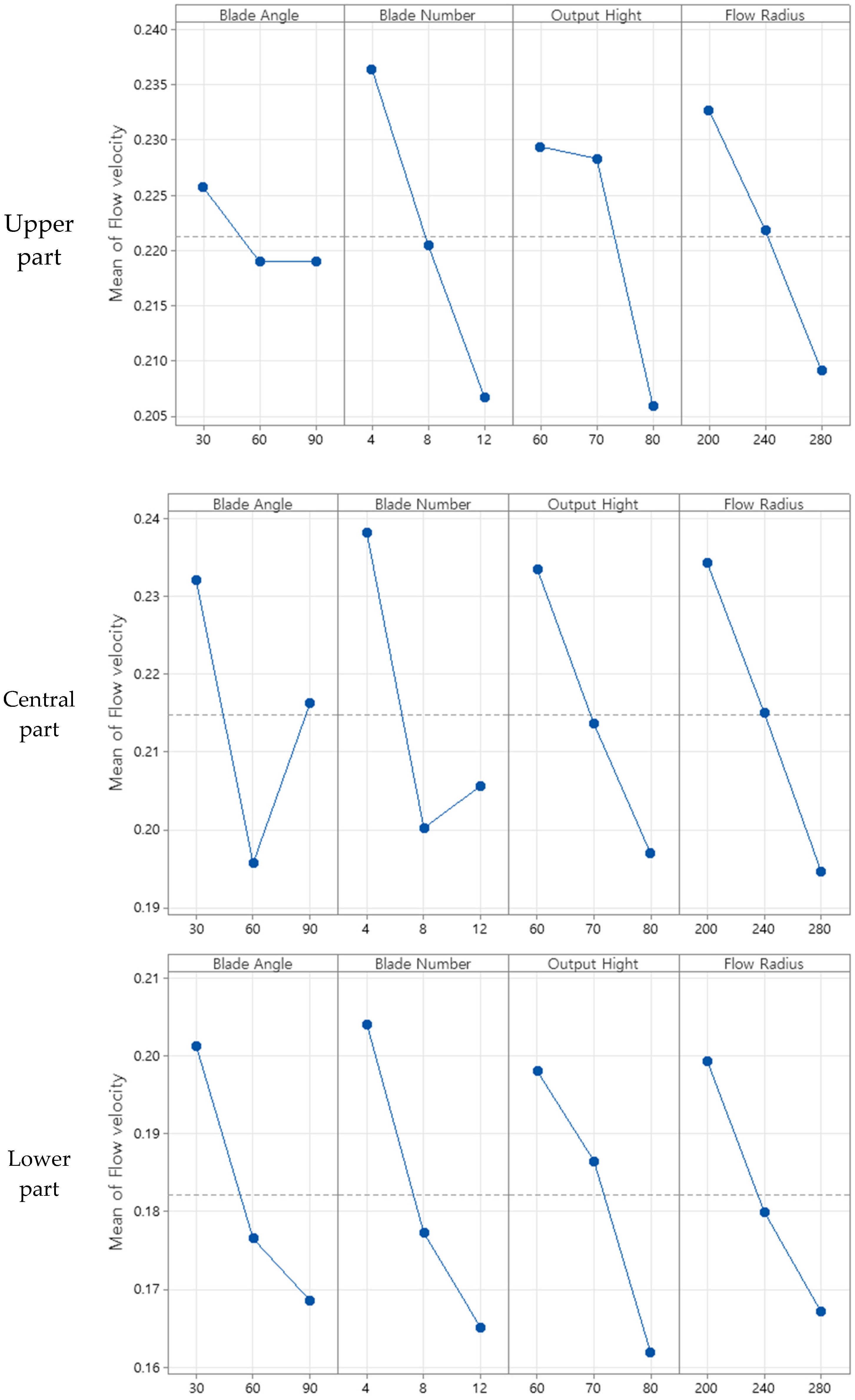
3.2. Application of the Taguchi Method
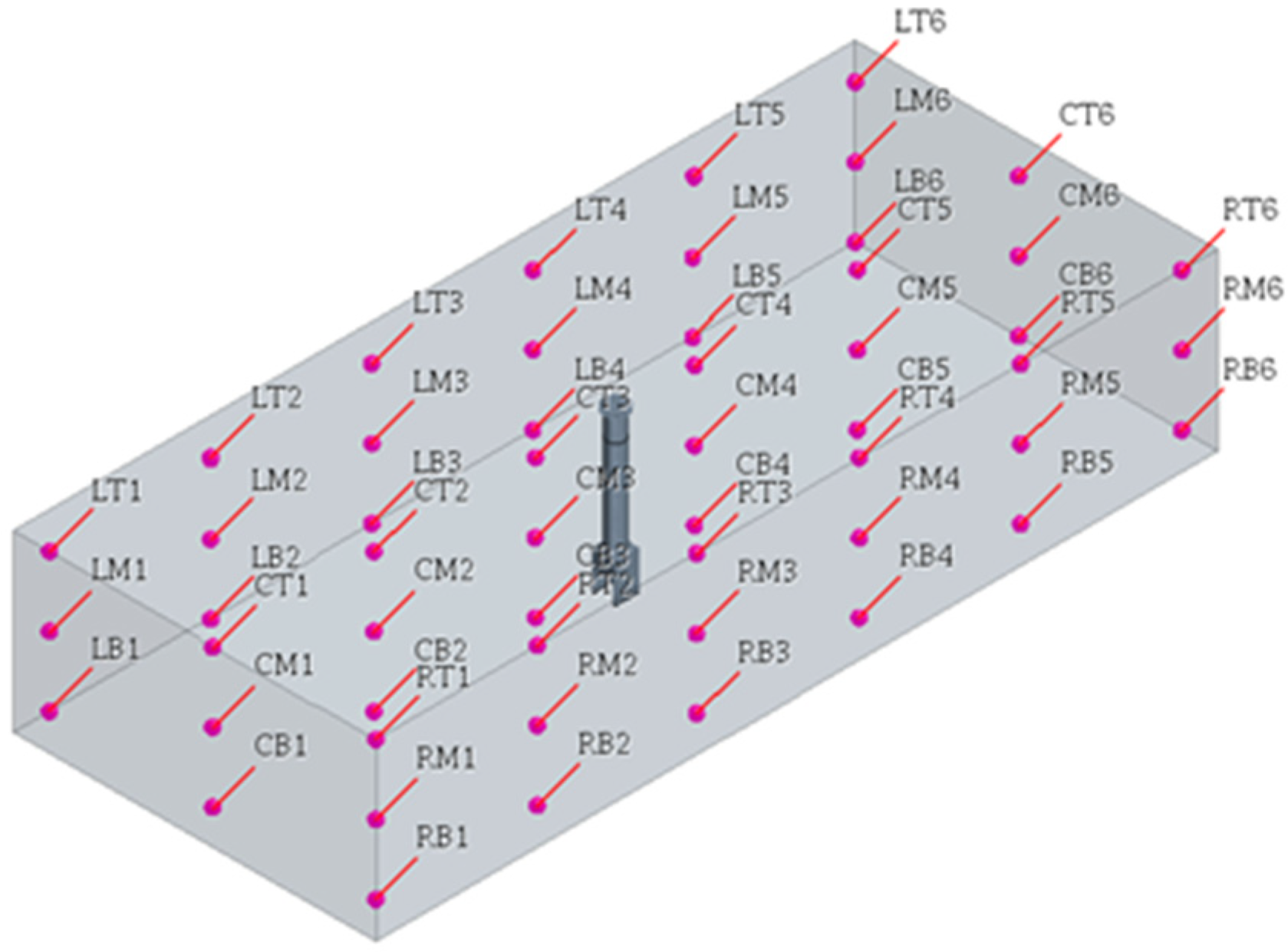
3.3. Analysis Grid and Conditions
- (1)
- Generation of the Analysis Grid
- (2)
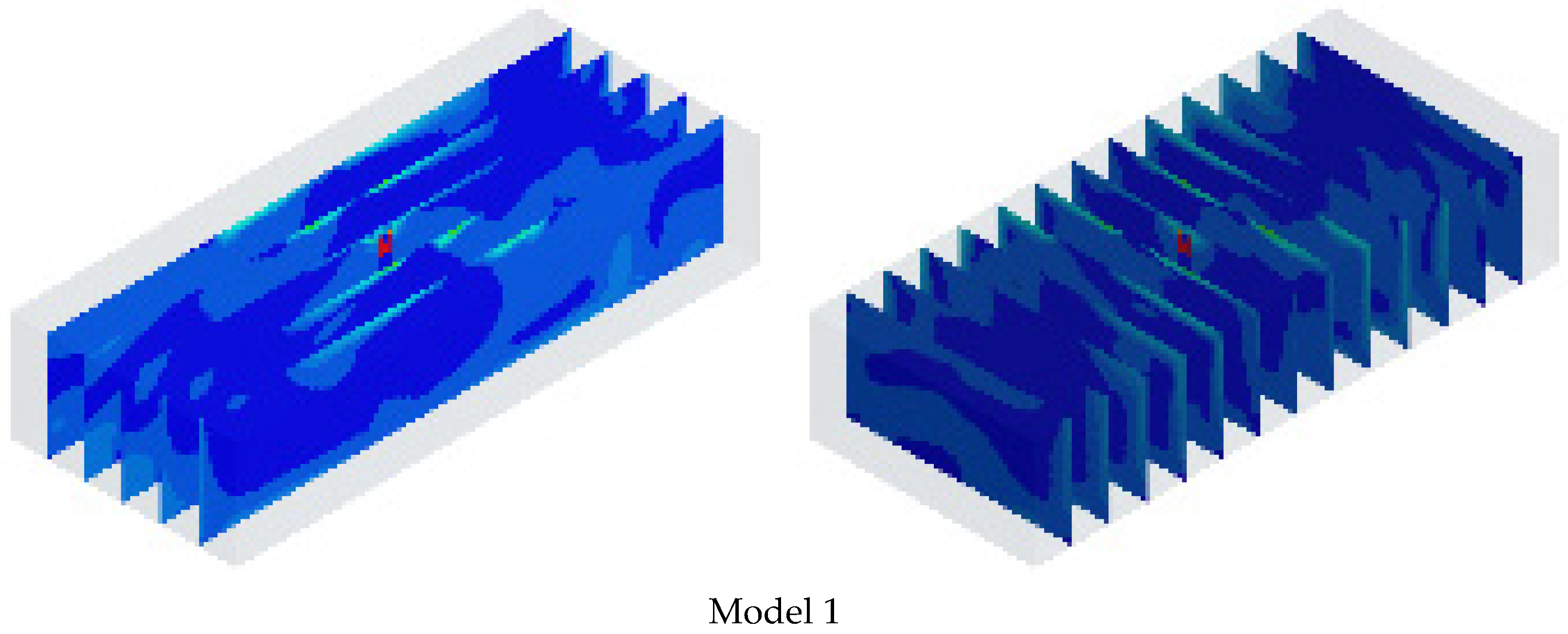
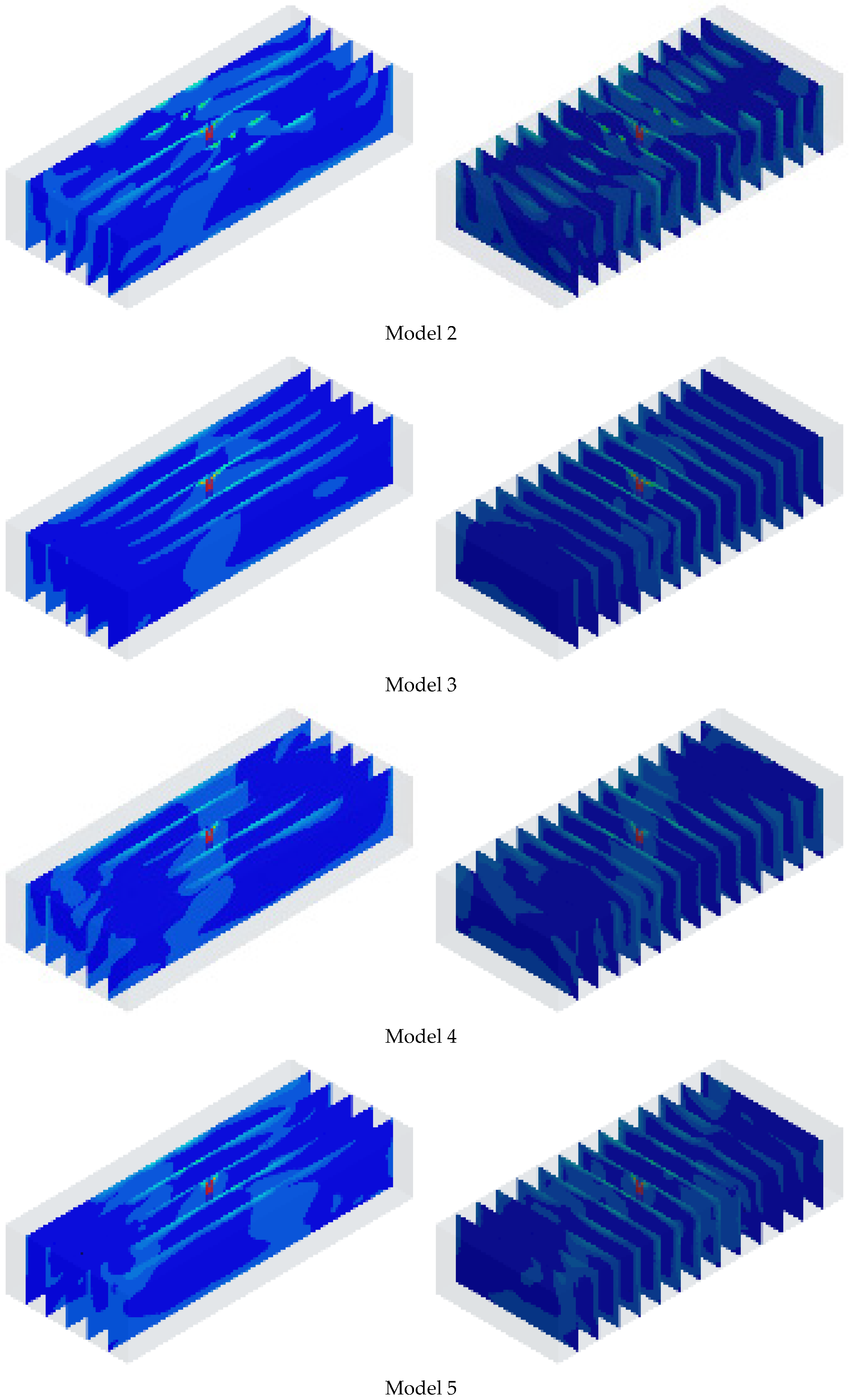
- Analysis Conditions and Results
4. Experimental Apparatus and Methods
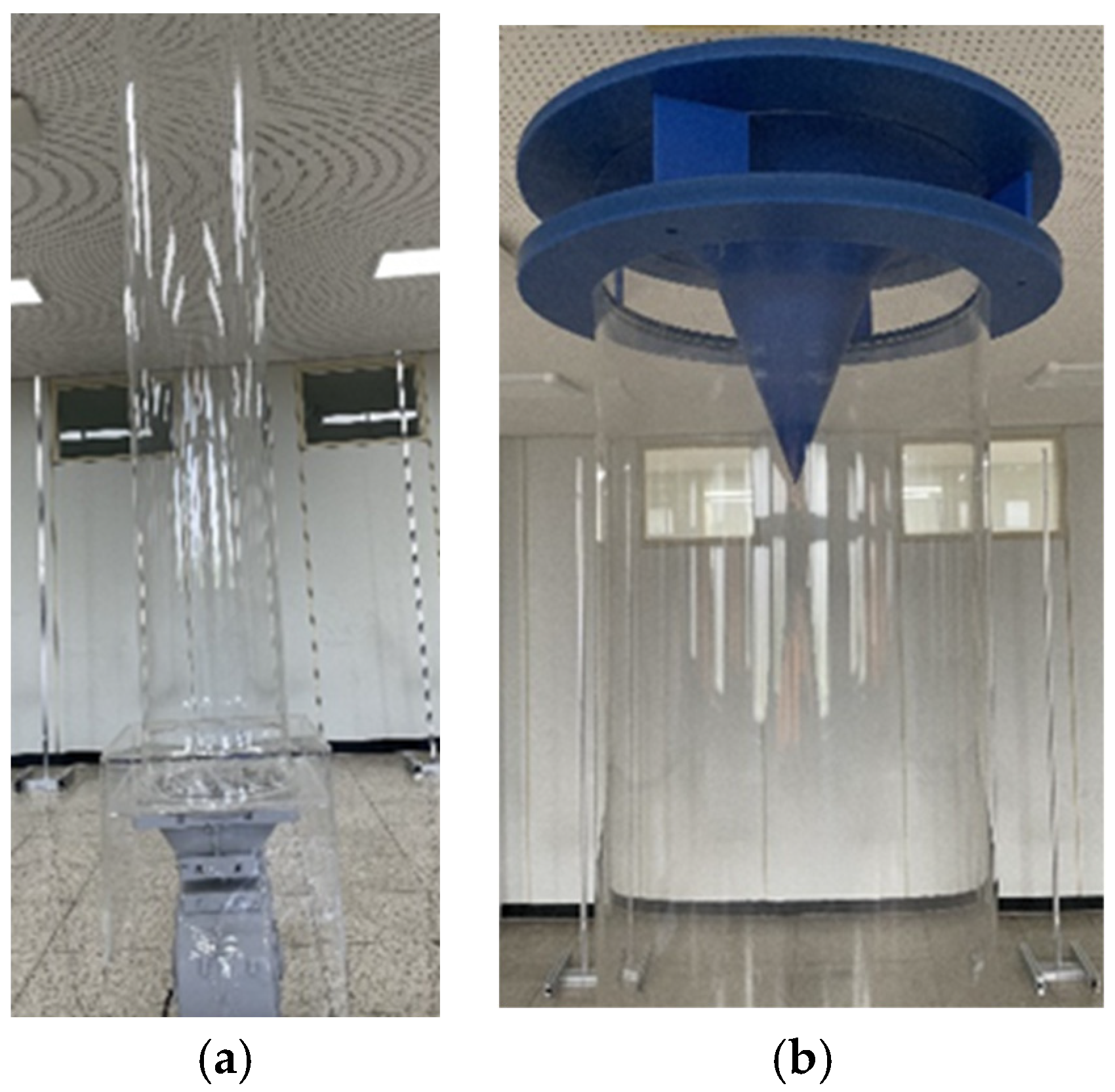
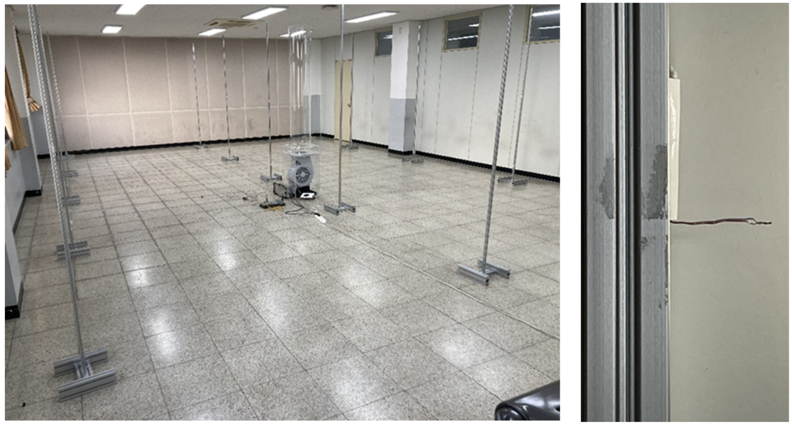
4.1. Experimental Apparatus
4.2. Experimental Methods
5. Results and Discussion
5.1. Air Circulation by Natural Convection
5.2. Model without an Outlet Shape
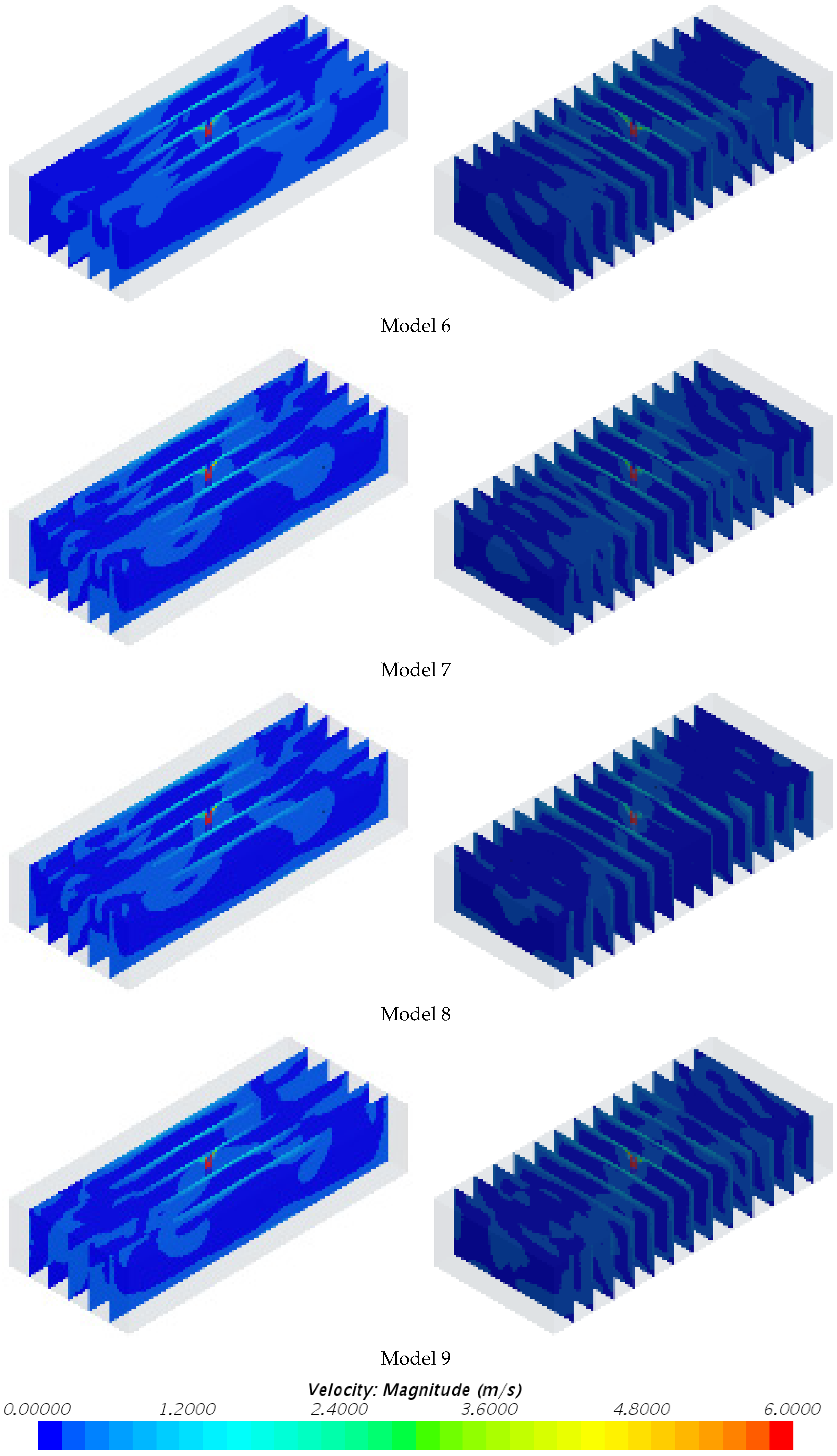
5.3. Model with an Outlet Shape
6. Conclusions
Author Contributions
Funding
Institutional Review Board Statement
Informed Consent Statement
Data Availability Statement
Conflicts of Interest
References
- Lee, J.W. Implemented Low-Cost Smart Farm Control System Using Arduino; Department of Electronics and Computer Engineering, Graduate School of Industry and Technology, Chonnam National University: Gwangju, Republic of Korea, 2019. [Google Scholar]
- Kim, M.J. Effects of ICT (Smart Farm) Application to Temperature, Humidity and Nutrient Solution Control on the Growth of Cherry Tomato and Reduced Labour; Department of Horticulture, Graduate School of Kongju National University: Gwangju, Republic of Korea, 2019. [Google Scholar]
- Yu, I.H.; Cho, M.W.; Lee, S.Y.; Chum, H.; Lee, I.B. Effects of Circulation Fans on Uniformity of Meteorological Factors in Warm Air Heated Greenhouse. J. Bio-Environ. Control. 2005, 14, 291–296. [Google Scholar]
- Muangprathub, J.; Boonnam, N.; Kajornkasirat, S.; Lekbangpong, N.; Wanichsombat, A.; Nillaor, P. IoT and agriculture data analysis for smart farm. Comput. Electron. Agric. 2019, 156, 467–474. [Google Scholar] [CrossRef]
- Ho, J. A Study on the Heat Transfer Characteristics of Thermal Storage Roof with the Air Circulation System; Department of Architecture Engineering, Graduate School, Taejon University: Daejeon, Republic of Korea, 2000. [Google Scholar]
- Culibrina, F.B.; Dadios, E.P. Smart farm using wireless sensor network for data acquisition and power control distribution. In Proceedings of the 2015 International Conference on Humanoid, Nanotechnology, Information Technology, Communication and Control, Environment and Management (HNICEM), Cebu, Philippines, 9–12 December 2015; IEEE: Piscataway, NJ, USA, 2015; pp. 1–6. [Google Scholar]
- Ministry of Agriculture Food and Rural Affairs in South Korea. Self-Assessment Report (Main Policy Section); Ministry of Agriculture Food and Rural Affairs in South Korea: Yeongi-gun, Republic of Korea, 2021. [Google Scholar]
- Korea Agribusiness Research Institute. Agricultural Management Consulting Performance Survey Analysis Final Report; Korea Agribusiness Research Institute: Ansan-si, Republic of Korea, 2019. [Google Scholar]
- Park, S.H. Study of Development of Thermal Storage Roof with the Air Circulation System; Department of Architectural Engineering, Graduate School, Daejeon University: Daejeon, Republic of Korea, 2002. [Google Scholar]
- Yoon, J.H.; Lee, C.S.; Kim, H.J.; Park, J.W.; Shin, U.C. A Study on Estimating Reduction of Heating Energy and CO by Indoor Setting Temperature with Clo; The Korean Solar Energy Society: Seoul, Republic of Korea, 2009; pp. 115–120. [Google Scholar]
- Yoon, J.S. Establishing the Comfort Zone of Thermal Environment in Winter. J. Korean Home Econ. Assoc. 1992, 30, 81–86. [Google Scholar]
- Kim, S.W.; Lee, S.; Kim, D.G. A Study of Thermal Comfort by Winter Temperature Humidity Change. Korean J. Air-Cond. Refrig. Eng. 2007, 19, 803–809. [Google Scholar]
- Rhee, K.N.; Jung, G.J. Experimental Study on the Improvement of Ventilation Performance and Thermal Environment using Air Circulators. J. Korean Inst. Archit. Sustain. Environ. Build. Syst. 2018, 12, 212–222. [Google Scholar]
- Kang, J.W. Parameter Optimization in Chamber Design of Exhaust System with Taguchi Method; Department of Automotive Engineering, Graduate School, University of Ulsan: Ulsan, Republic of Korea, 2008. [Google Scholar]
- Kuroyanagi, T. Current usage of air circulators in greenhouses in Japan. Jpn. Agric. Res. Q. 2016, 50, 7–12. [Google Scholar] [CrossRef] [Green Version]
- Murakami, S.; Kato, S. New scales for ventilation efficiency and their application based on numerical simulation of room airflow. In Proceedings of the International Symposium on Room Air Convection and Ventilation Effectiveness, Tokyo, Japan, 22–24 July 1992; University of Tokyo: Tokyo, Japan, 1992; pp. 22–38. [Google Scholar]
- Ramya, R.; Sandhya, C.; Shwetha, R. Smart farming systems using sensors. In Proceedings of the 2017 IEEE Technological Innovations in ICT for Agriculture and Rural Development (TIAR), Chennai, India, 7–8 April 2017; IEEE: Piscataway, NJ, USA, 2017; pp. 218–222. [Google Scholar]
- Kim, B.J. Inlet & Outlet Port Shape Optimization of GeRotor Pump; Department of Mechanical Engineering, Graduate School, Pusan National University: Busan, Republic of Korea, 2006. [Google Scholar]
- Park, J.K. A Study on the Ventilation Efficiency Evaluation of the Combined Air-Diffuser Ventilation System Using CFD; The Department of Architecture, Graduate School, Yeungnam University: Gyeongsan, Republic of Korea, 2017. [Google Scholar]
- Kim, M.J. Differences in Skin Temperature and Perceived Thermal Comfort Based on Age, Sex and Clothing Weight of Participants in a Room at Recommended Room Temperature. Korean J. Community Living Sci. 2004, 15, 55–64. [Google Scholar]
- Cheboxarov, V. Vertical air circulation in a low-speed lateral flow wind turbine with rotary blades. Tech. Phys. Lett. 2008, 34, 52–55. [Google Scholar] [CrossRef]
- Lim, R. Analysis on the Temperature and Humidity in Greenhouse by the Operation of Air Circulation Fan and Foggging System. J. Korean Soc. Agric. Mach. 2020, 25, 178. [Google Scholar]
- Lee, T.S.; Kang, G.C.; Jang, J.K.; Paek, Y.; Lim, R.G. Analysis on the Effect of Greenhouse Humidity Control by Counter-flow Ventilator in Winter. Prot. Hortic. Plant Fact. 2020, 29, 259–264. [Google Scholar] [CrossRef]
- Koh, J.Y.; Kim, I.G.; Choi, B.H.; Yim, C.S. A Numerical Analysis on Forced Ventilation using Indoor Air Cleaner in an Apartment House. Int. J. Air-Cond. Refrig. Eng. 2001, 13, 217–224. [Google Scholar]
- Hwang, S.D.; Cho, H.H. Flow and Heat Transfer Characteristics of a Multi-Tube Inserted Impinging Jet. Trans. Korean Soc. Mech. Eng. 2004, 28, 135–145. [Google Scholar]
- Jang, W.G. Optimal Design of the Front Upright of Formula Race Car Using Taguchi’s Orthogonal Array. J. Korean Soc. Manuf. Technol. Eng. 2013, 22, 112–118. [Google Scholar]
- Son, J.-H.; Cho, D.-H.; Nah, K.-D. A Study on the Air Flow Velocity and Temperature Distribution Characteristics of Hybrid Smart Farm. Adv. Sci. Technol. Lett. 2016, 140, 110–117. [Google Scholar]
- Park, S.H. A Study on the Performance Improvement of Supply and Exhaust Integrated Ventilation System; Department of Design and Engineering, Graduate School of Nano IT Design Fusion, Seoul National University of Science and Technology: Seoul, Republic of Korea, 2020. [Google Scholar]
- Versteeg, H.K.; Malalasekera, W. An Introduction to Computational Fluid Dynamics: The Finite Volume Method; Pearson Education: London, UK, 2007. [Google Scholar]
- Cd-Adapco, S. STAR CCM+ User Guide Version 12.04; CD-Adapco: New York, NY, USA, 2017; p. 62. [Google Scholar]
- MINITAB. Minitab User’s Guide. Available online: http://www.personal.psu.edu/klm47/Courses/STAT250/Fall2015/minitab.pdf (accessed on 1 February 2023).
- SYSTÈMES, Dassault. CATIA V5 User Guides. Part Design, Assebmly Design, Wireframe and Surface, Version. Available online: http://catiadoc.free.fr/online/CATIAfr_C2/prtugCATIAfrs.htm (accessed on 1 February 2023).
- Yoon, H.J.; Ham, I.T.; Kim, J.S.; Choi, J.D. Optimization of the Manufacturing Process for Boiled-dried Anchovy Using Response Surface Methodology (RSM). J. Fish. Mar. Sci. Educ. 2017, 29, 1984–1993. [Google Scholar]
- Shetty, P.K.; Shetty, R.; Shetty, D.; Rehaman, N.F.; Jose, T.K. Machinability study on dry drilling of titanium alloy Ti-6Al-4V using L9 orthoganal array. Procedia Mater. Sci. 2014, 5, 2605–2614. [Google Scholar] [CrossRef] [Green Version]


| Factor | Blade Angle [°] | Blade Number [ea] | Output Height [mm] | Flow Radius [mm] | |
|---|---|---|---|---|---|
| Level | |||||
| 1 | 30 | 4 | 60 | 200 | |
| 2 | 60 | 8 | 70 | 240 | |
| 3 | 90 | 12 | 80 | 280 | |
| Exp. | Blade Angle [°] | Blade Number [ea] | Output Height [mm] | Flow Radius [mm] |
|---|---|---|---|---|
| 1 | 30 | 4 | 60 | 200 |
| 2 | 30 | 8 | 70 | 240 |
| 3 | 30 | 12 | 80 | 280 |
| 4 | 60 | 4 | 70 | 280 |
| 5 | 60 | 8 | 80 | 200 |
| 6 | 60 | 12 | 60 | 240 |
| 7 | 90 | 4 | 80 | 240 |
| 8 | 90 | 8 | 60 | 280 |
| 9 | 90 | 12 | 70 | 200 |
| Part | Properties | Value |
|---|---|---|
| Fluid Region | Mesh Type | polyhedral |
| Base Size [mm] | 20 | |
| Number of Prism Layers [-] | 3 | |
| Prism Layer Thickness [mm] | 0.25 | |
| Minimum Surface Size [mm] | 0.5 |
| Units: m/s | |||||||||
|---|---|---|---|---|---|---|---|---|---|
| Mod.1 | Mod.2 | Mod.3 | Mod.4 | Mod.5 | Mod.6 | Mod.7 | Mod.8 | Mod.9 | |
| LT1 | 0.228 | 0.280 | 0.224 | 0.344 | 0.121 | 0.069 | 0.144 | 0.120 | 0.161 |
| LT2 | 0.113 | 0.777 | 0.340 | 0.368 | 0.323 | 0.226 | 0.244 | 0.333 | 0.268 |
| LT3 | 0.333 | 0.094 | 0.204 | 0.306 | 0.355 | 0.232 | 0.334 | 0.373 | 0.350 |
| LT4 | 0.255 | 0.210 | 0.355 | 0.352 | 0.351 | 0.372 | 0.341 | 0.241 | 0.343 |
| LT5 | 0.570 | 0.143 | 0.183 | 0.261 | 0.195 | 0.281 | 0.360 | 0.407 | 0.299 |
| LT6 | 0.206 | 0.192 | 0.057 | 0.125 | 0.163 | 0.131 | 0.128 | 0.149 | 0.269 |
| CT1 | 0.125 | 0.258 | 0.017 | 0.199 | 0.144 | 0.153 | 0.199 | 0.107 | 0.145 |
| CT2 | 0.162 | 0.386 | 0.097 | 0.079 | 0.120 | 0.165 | 0.126 | 0.103 | 0.083 |
| CT3 | 0.187 | 0.137 | 0.136 | 0.112 | 0.141 | 0.174 | 0.134 | 0.085 | 0.134 |
| CT4 | 0.167 | 0.131 | 0.181 | 0.125 | 0.142 | 0.125 | 0.138 | 0.094 | 0.138 |
| CT5 | 0.156 | 0.057 | 0.194 | 0.092 | 0.123 | 0.095 | 0.071 | 0.133 | 0.090 |
| CT6 | 0.208 | 0.141 | 0.084 | 0.071 | 0.155 | 0.170 | 0.167 | 0.123 | 0.176 |
| RT1 | 0.263 | 0.033 | 0.094 | 0.138 | 0.186 | 0.151 | 0.151 | 0.156 | 0.124 |
| RT2 | 0.551 | 0.213 | 0.230 | 0.261 | 0.263 | 0.317 | 0.346 | 0.359 | 0.327 |
| RT3 | 0.239 | 0.189 | 0.198 | 0.392 | 0.387 | 0.369 | 0.311 | 0.279 | 0.302 |
| RT4 | 0.598 | 0.106 | 0.315 | 0.234 | 0.332 | 0.272 | 0.332 | 0.262 | 0.325 |
| RT5 | 0.131 | 0.670 | 0.312 | 0.468 | 0.253 | 0.363 | 0.265 | 0.396 | 0.350 |
| RT6 | 0.197 | 0.171 | 0.091 | 0.199 | 0.107 | 0.175 | 0.161 | 0.139 | 0.132 |
| mean | 0.26 | 0.23 | 0.18 | 0.23 | 0.21 | 0.21 | 0.22 | 0.21 | 0.22 |
| Units: m/s | |||||||||
|---|---|---|---|---|---|---|---|---|---|
| Mod.1 | Mod.2 | Mod.3 | Mod.4 | Mod.5 | Mod.6 | Mod.7 | Mod.8 | Mod.9 | |
| LM1 | 0.263 | 0.296 | 0.250 | 0.303 | 0.129 | 0.144 | 0.178 | 0.174 | 0.142 |
| LM2 | 0.339 | 0.315 | 0.221 | 0.179 | 0.128 | 0.221 | 0.243 | 0.314 | 0.234 |
| LM3 | 0.305 | 0.262 | 0.180 | 0.163 | 0.257 | 0.234 | 0.257 | 0.163 | 0.230 |
| LM4 | 0.267 | 0.254 | 0.250 | 0.228 | 0.213 | 0.195 | 0.181 | 0.141 | 0.205 |
| LM5 | 0.383 | 0.274 | 0.130 | 0.291 | 0.220 | 0.271 | 0.290 | 0.291 | 0.289 |
| LM6 | 0.325 | 0.216 | 0.120 | 0.217 | 0.200 | 0.171 | 0.199 | 0.195 | 0.225 |
| CM1 | 0.287 | 0.205 | 0.089 | 0.177 | 0.172 | 0.188 | 0.254 | 0.205 | 0.277 |
| CM2 | 0.301 | 0.198 | 0.175 | 0.094 | 0.147 | 0.194 | 0.191 | 0.183 | 0.196 |
| CM3 | 0.322 | 0.157 | 0.233 | 0.237 | 0.254 | 0.087 | 0.225 | 0.116 | 0.189 |
| CM4 | 0.283 | 0.184 | 0.254 | 0.193 | 0.120 | 0.165 | 0.200 | 0.123 | 0.227 |
| CM5 | 0.269 | 0.089 | 0.182 | 0.069 | 0.199 | 0.159 | 0.170 | 0.179 | 0.197 |
| CM6 | 0.266 | 0.093 | 0.136 | 0.175 | 0.088 | 0.255 | 0.185 | 0.278 | 0.273 |
| RM1 | 0.335 | 0.057 | 0.145 | 0.186 | 0.222 | 0.181 | 0.186 | 0.181 | 0.201 |
| RM2 | 0.352 | 0.213 | 0.124 | 0.175 | 0.179 | 0.242 | 0.282 | 0.268 | 0.263 |
| RM3 | 0.157 | 0.266 | 0.272 | 0.198 | 0.237 | 0.225 | 0.228 | 0.108 | 0.235 |
| RM4 | 0.349 | 0.216 | 0.245 | 0.126 | 0.291 | 0.245 | 0.278 | 0.092 | 0.217 |
| RM5 | 0.291 | 0.308 | 0.178 | 0.299 | 0.041 | 0.311 | 0.277 | 0.369 | 0.297 |
| RM6 | 0.194 | 0.302 | 0.154 | 0.257 | 0.202 | 0.218 | 0.179 | 0.231 | 0.167 |
| mean | 0.29 | 0.21 | 0.19 | 0.21 | 0.20 | 0.23 | 0.25 | 0.23 | 0.27 |
| Units: m/s | |||||||||
|---|---|---|---|---|---|---|---|---|---|
| Mod.1 | Mod.2 | Mod.3 | Mod.4 | Mod.5 | Mod.6 | Mod.7 | Mod.8 | Mod.9 | |
| LB1 | 0.164 | 0.157 | 0.126 | 0.154 | 0.065 | 0.075 | 0.110 | 0.145 | 0.101 |
| LB2 | 0.399 | 0.259 | 0.163 | 0.157 | 0.075 | 0.147 | 0.180 | 0.259 | 0.161 |
| LB3 | 0.271 | 0.272 | 0.192 | 0.185 | 0.201 | 0.179 | 0.212 | 0.162 | 0.190 |
| LB4 | 0.177 | 0.237 | 0.205 | 0.199 | 0.238 | 0.222 | 0.189 | 0.124 | 0.189 |
| LB5 | 0.268 | 0.129 | 0.138 | 0.267 | 0.245 | 0.228 | 0.215 | 0.184 | 0.173 |
| LB6 | 0.240 | 0.103 | 0.070 | 0.066 | 0.126 | 0.136 | 0.171 | 0.181 | 0.183 |
| CB1 | 0.382 | 0.148 | 0.202 | 0.305 | 0.265 | 0.214 | 0.184 | 0.098 | 0.234 |
| CB2 | 0.159 | 0.215 | 0.173 | 0.185 | 0.215 | 0.168 | 0.133 | 0.130 | 0.095 |
| CB3 | 0.292 | 0.126 | 0.144 | 0.127 | 0.122 | 0.251 | 0.115 | 0.189 | 0.193 |
| CB4 | 0.176 | 0.154 | 0.132 | 0.173 | 0.129 | 0.210 | 0.152 | 0.133 | 0.230 |
| CB5 | 0.180 | 0.290 | 0.179 | 0.192 | 0.212 | 0.115 | 0.131 | 0.111 | 0.142 |
| CB6 | 0.334 | 0.276 | 0.146 | 0.349 | 0.156 | 0.038 | 0.088 | 0.216 | 0.102 |
| RB1 | 0.226 | 0.036 | 0.081 | 0.207 | 0.128 | 0.111 | 0.154 | 0.172 | 0.169 |
| RB2 | 0.272 | 0.174 | 0.036 | 0.142 | 0.209 | 0.196 | 0.196 | 0.170 | 0.175 |
| RB3 | 0.169 | 0.174 | 0.210 | 0.167 | 0.252 | 0.232 | 0.192 | 0.104 | 0.188 |
| RB4 | 0.287 | 0.261 | 0.222 | 0.123 | 0.213 | 0.203 | 0.215 | 0.125 | 0.220 |
| RB5 | 0.385 | 0.361 | 0.202 | 0.206 | 0.093 | 0.186 | 0.208 | 0.282 | 0.212 |
| RB6 | 0.230 | 0.203 | 0.063 | 0.177 | 0.093 | 0.207 | 0.183 | 0.178 | 0.159 |
| mean | 0.26 | 0.20 | 0.15 | 0.19 | 0.17 | 0.17 | 0.17 | 0.16 | 0.17 |
| Level | Blade Angle | Blade Number | Output Height | Flow Radius |
|---|---|---|---|---|
| 1 | 0.2257 | 0.2364 | 0.2294 | 0.2327 |
| 2 | 0.2190 | 0.2205 | 0.2283 | 0.2219 |
| 3 | 0.2190 | 0.2068 | 0.2060 | 0.2092 |
| Delta | 0.0067 | 0.0296 | 0.0234 | 0.0235 |
| Rank | 4 | 1 | 3 | 2 |
| Level | Blade Angle | Blade Number | Output Height | Flow Radius |
|---|---|---|---|---|
| 1 | 0.2321 | 0.2381 | 0.2334 | 0.2343 |
| 2 | 0.1958 | 0.2003 | 0.2136 | 0.2151 |
| 3 | 0.2163 | 0.2057 | 0.1970 | 0.1947 |
| Delta | 0.0363 | 0.0378 | 0.0364 | 0.0395 |
| Rank | 4 | 2 | 3 | 1 |
| Level | Blade Angle | Blade Number | Output Height | Flow Radius |
|---|---|---|---|---|
| 1 | 0.2013 | 0.2041 | 0.1980 | 0.1993 |
| 2 | 0.1766 | 0.1773 | 0.1865 | 0.1800 |
| 3 | 0.1686 | 0.1651 | 0.1620 | 0.1672 |
| Delta | 0.0326 | 0.0389 | 0.0360 | 0.0321 |
| Rank | 3 | 1 | 2 | 4 |
Disclaimer/Publisher’s Note: The statements, opinions and data contained in all publications are solely those of the individual author(s) and contributor(s) and not of MDPI and/or the editor(s). MDPI and/or the editor(s) disclaim responsibility for any injury to people or property resulting from any ideas, methods, instructions or products referred to in the content. |
© 2023 by the authors. Licensee MDPI, Basel, Switzerland. This article is an open access article distributed under the terms and conditions of the Creative Commons Attribution (CC BY) license (https://creativecommons.org/licenses/by/4.0/).
Share and Cite
Park, J.-Y.; Yoo, Y.-J.; Kim, Y.-C. Optimization of the Outlet Shape of an Air Circulation System for Reduction of Indoor Temperature Difference. Sensors 2023, 23, 2570. https://doi.org/10.3390/s23052570
Park J-Y, Yoo Y-J, Kim Y-C. Optimization of the Outlet Shape of an Air Circulation System for Reduction of Indoor Temperature Difference. Sensors. 2023; 23(5):2570. https://doi.org/10.3390/s23052570
Chicago/Turabian StylePark, Jin-Young, Young-Jun Yoo, and Young-Choon Kim. 2023. "Optimization of the Outlet Shape of an Air Circulation System for Reduction of Indoor Temperature Difference" Sensors 23, no. 5: 2570. https://doi.org/10.3390/s23052570