
Remote Interference Discrimination Testbed Employing AI Ensemble Algorithms for 6G TDD Networks

Abstract
:1. Introduction
- A remote interference discrimination testbed is originally proposed, which adopts 5,520,000 TDD network-side interfered data to discriminate the remote interference. A large number of measurement data could effectively appraise the interference discrimination ability of different AI algorithms;
- The testbed verifies the interference discrimination ability of two types of a total of nine AI algorithms, which lays the foundation for the application of the testbed in different hardware environments;
- According to the consistent comparison, numerical results illustrate that the ensemble algorithm achieves an average accuracy of 12% higher than the single model algorithm. The work fills the gap of remote interference in the 6G communication scenario and helps mobile operators improve network optimization capabilities under remote interference.
2. Related Work and Testbed Design
2.1. Related Work
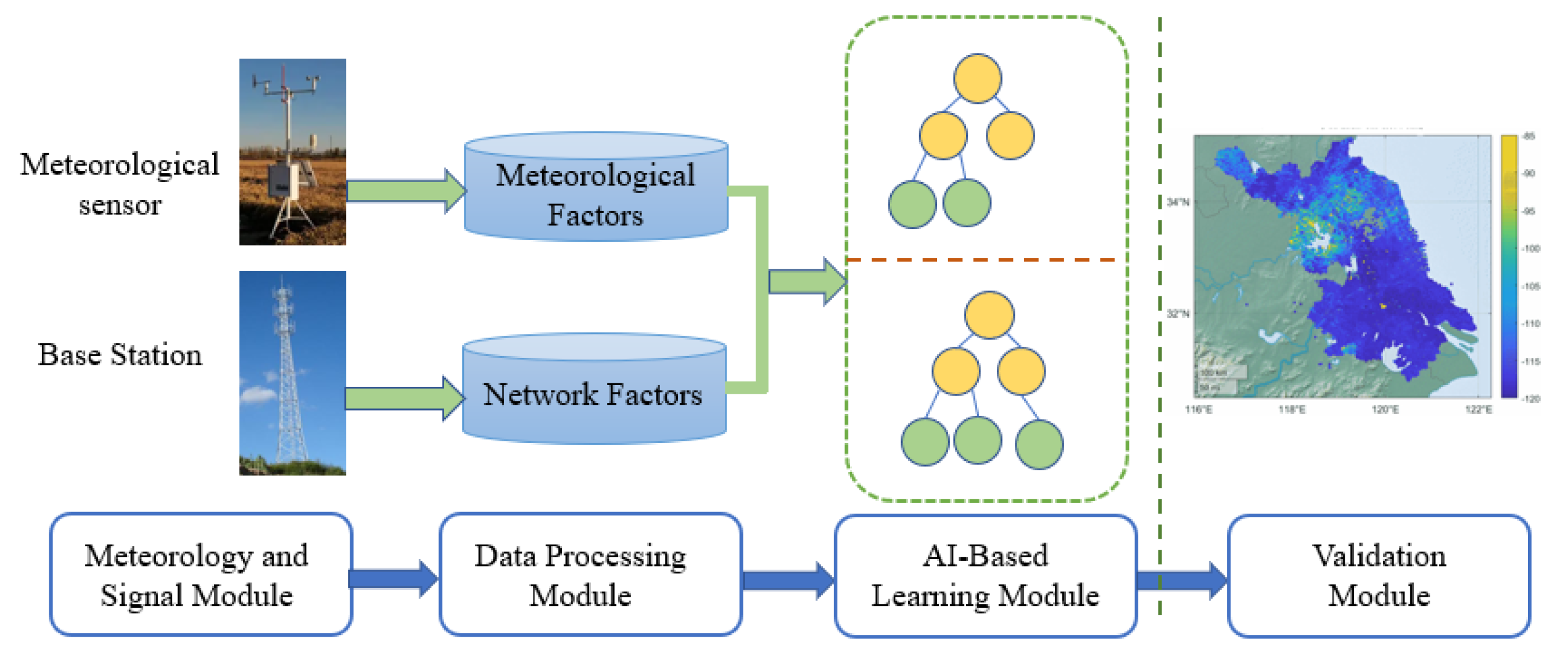
2.2. Testbed Design
2.2.1. Meteorological Factors
2.2.2. Network Factors
3. AI-Based Discriminant Algorithms
3.1. Single Model Algorithms
3.1.1. kNN
3.1.2. SVM
3.1.3. NB
3.2. Ensemble Algorithms
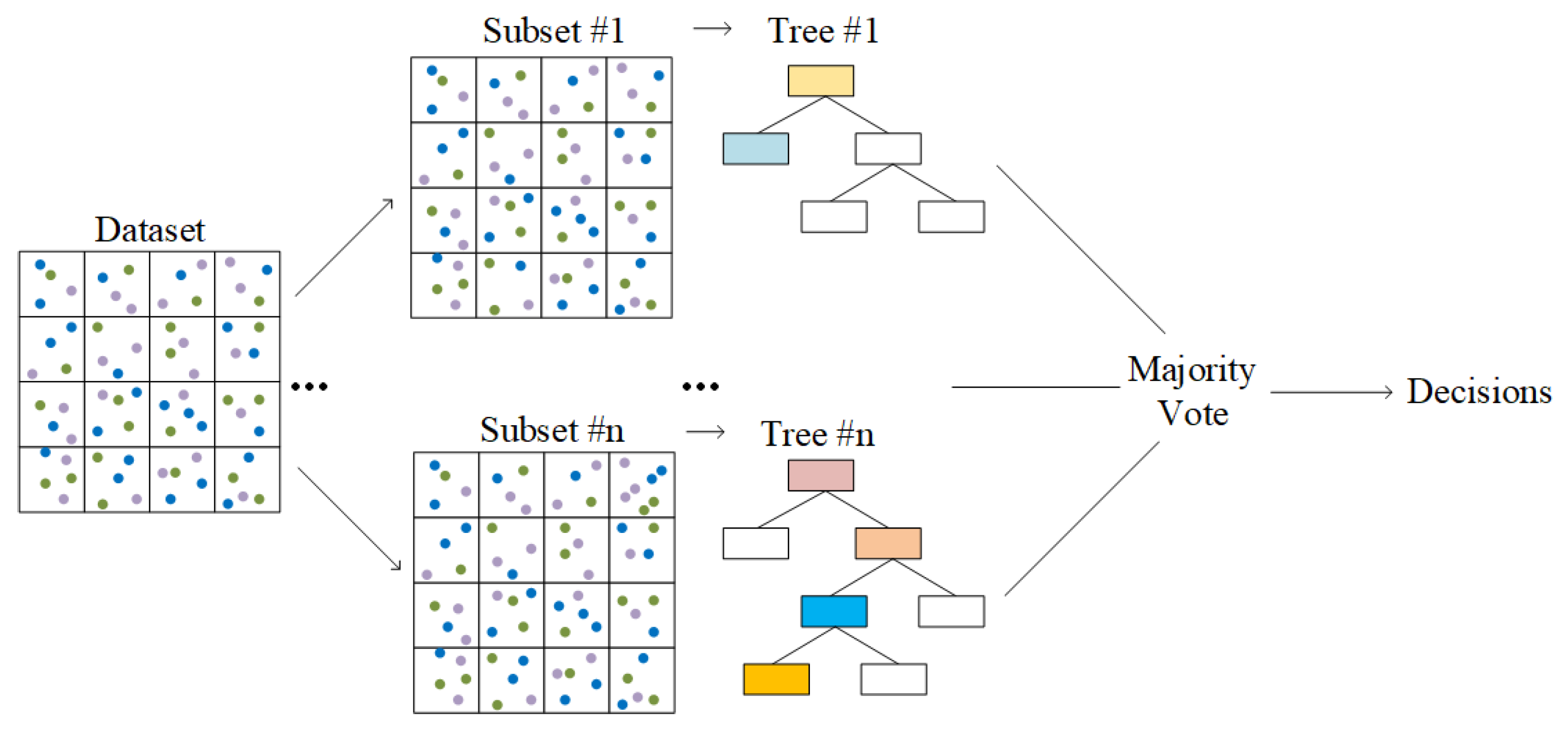
3.2.1. RF
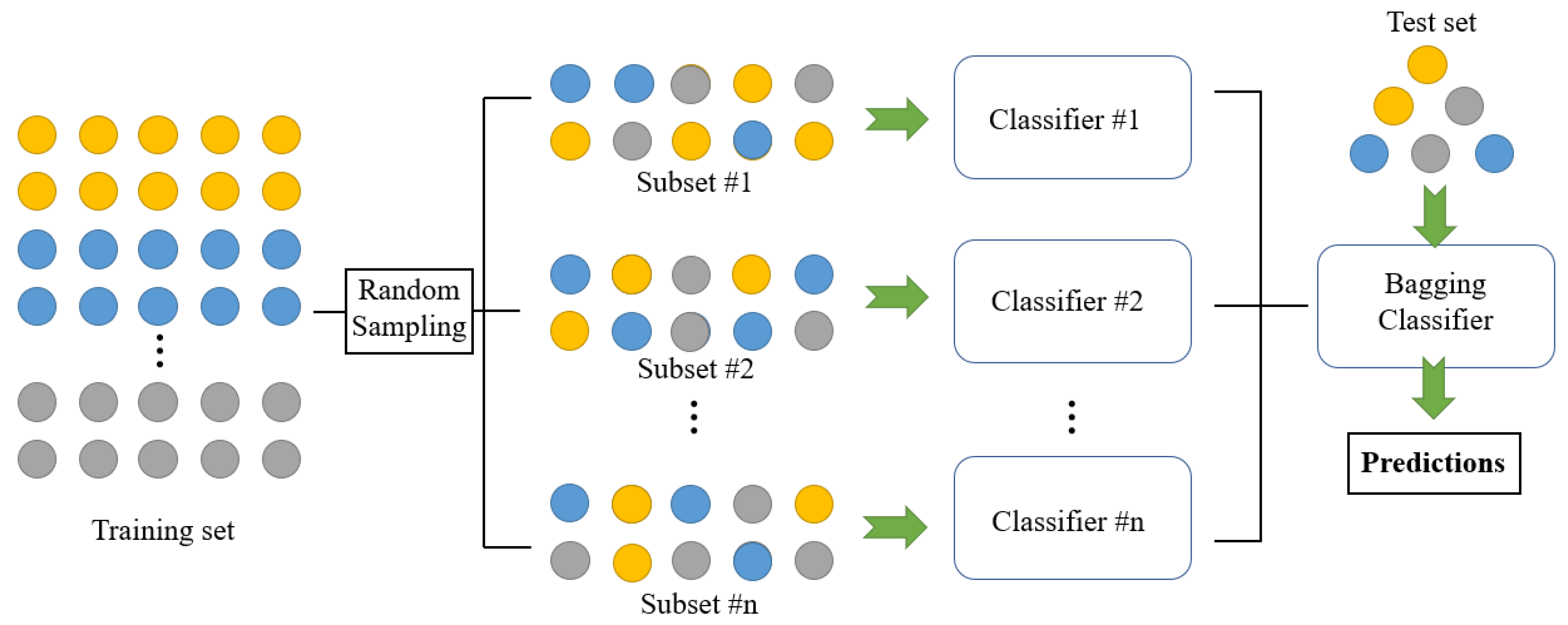
3.2.2. Bagging
3.2.3. Boosting
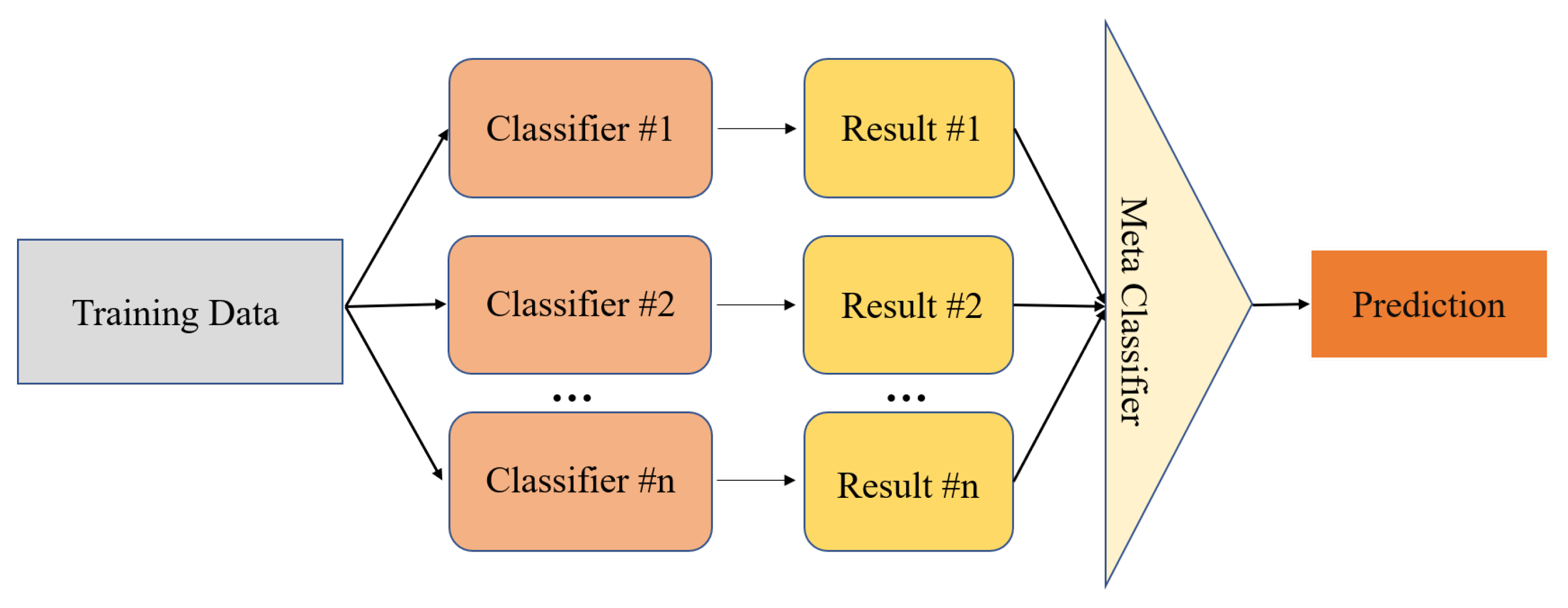
3.2.4. Stacking
4. Interference Discrimination Experiments
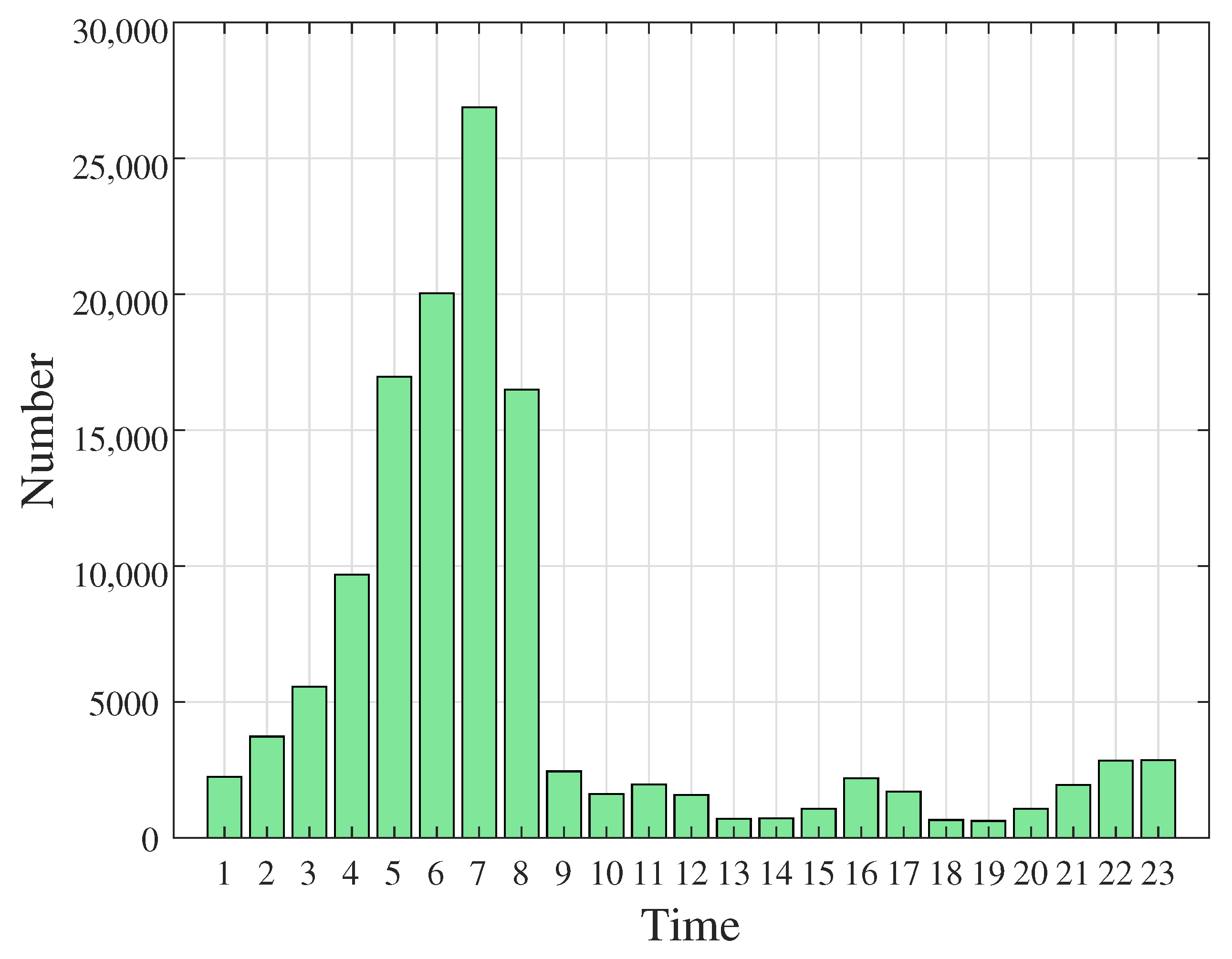
4.1. Interference Dataset
4.2. Algorithm Settings
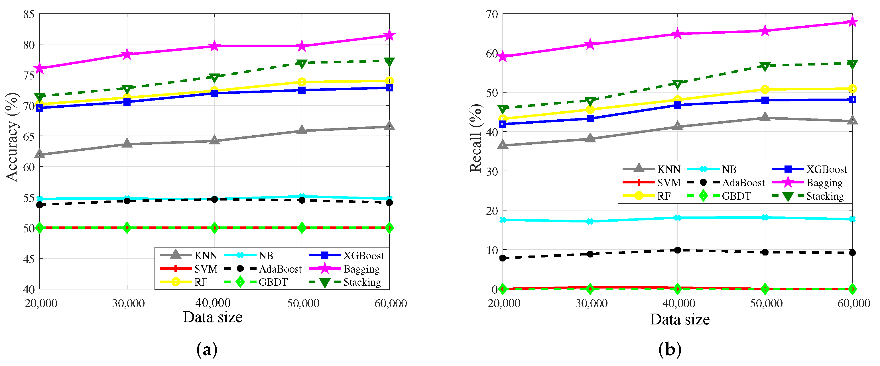
4.3. Sensitivity of the Algorithms to the Data Size
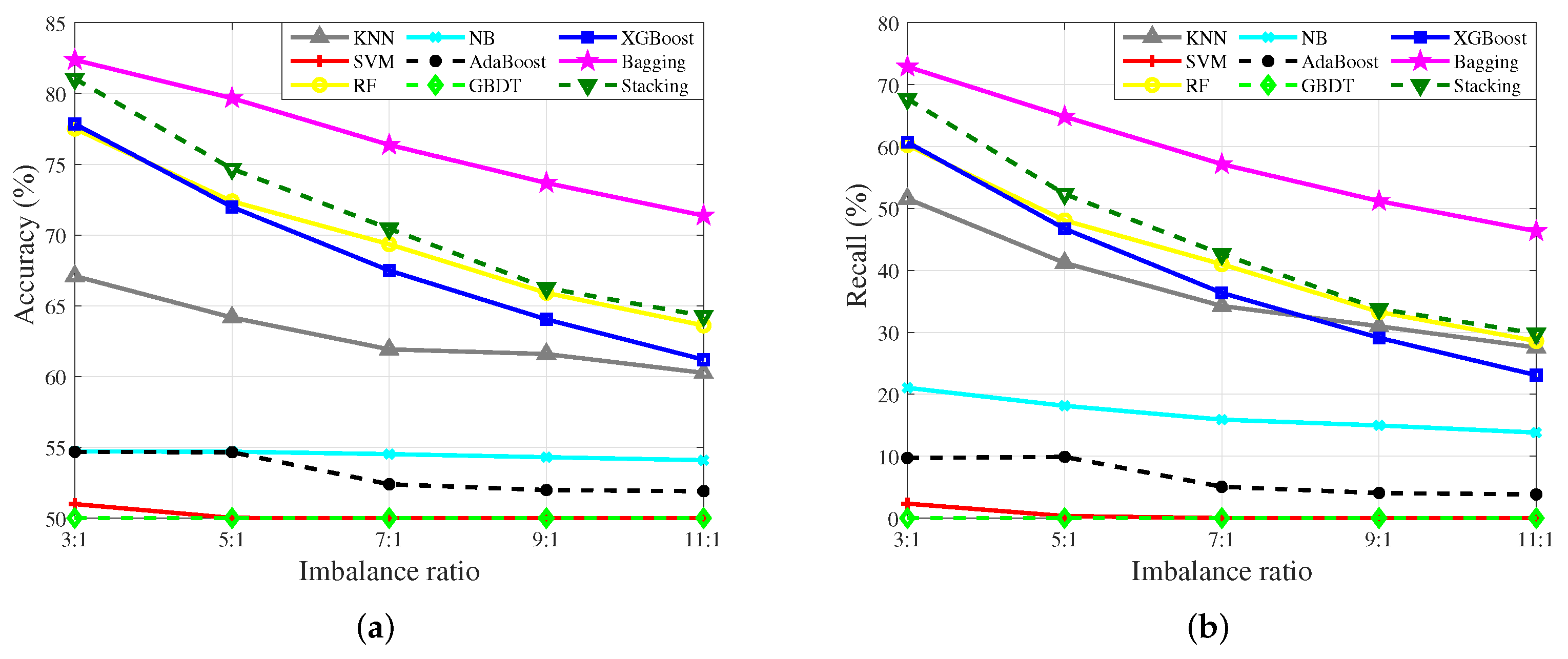
4.4. Sensitivity of the Algorithms to IR
4.5. Robustness Analysis of the Algorithms
4.6. Time Complexity
5. Conclusions
Author Contributions
Funding
Institutional Review Board Statement
Informed Consent Statement
Data Availability Statement
Conflicts of Interest
Abbreviations
| IoT | Internet of Things |
| TDD | Time-Division Duplex |
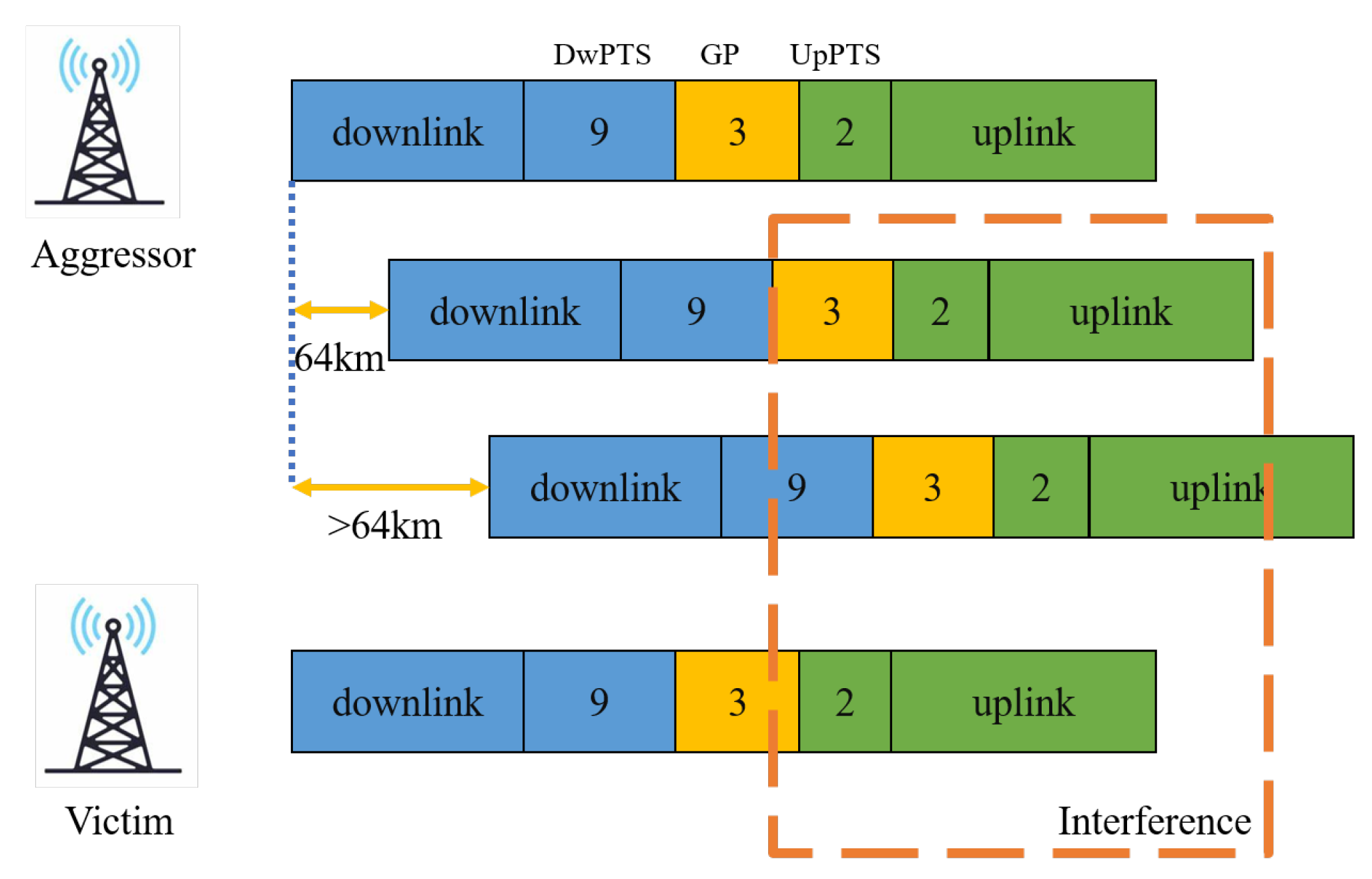
| GP | Guard Period |
| kNN | k-Nearest Neighbors |
| SVM | Support Vector Machine |
| NB | Naive Bayes |
| RF | Random Forest |
| AdaBoost | Adaptive Boosting |
| GBDT | Gradient Boosting Decision Tree |
| XGBoost | Xtreme Gradient Boosting |
| Bagging | Bootstrap Aggregating |
| Stacking | Stacked Generalization |
| PE | Parabolic Equation |
| IR | Imbalance Ratio |
References
- Chen, X.; Wu, C.; Chen, T.; Liu, Z.; Zhang, H.; Bennis, M.; Liu, H.; Ji, Y. Information Freshness-Aware Task Offloading in Air-Ground Integrated Edge Computing Systems. IEEE J. Sel. Areas Commun. 2022, 40, 243–258. [Google Scholar] [CrossRef]
- Cao, S.; Chen, X.; Zhang, X.; Chen, X. Improving the Tracking Accuracy of TDMA-Based Acoustic Indoor Positioning Systems Using a Novel Error Correction Method. IEEE Sens. J. 2022, 22, 5427–5436. [Google Scholar] [CrossRef]
- Xia, T.; Wang, M.M.; Zhang, J.; Wang, L. Maritime Internet of Things: Challenges and Solutions. IEEE Wirel. Commun. 2020, 27, 188–196. [Google Scholar] [CrossRef]
- Wagner, M.; Groll, H.; Dormiani, A.; Sathyanarayanan, V.; Mecklenbräuker, C.; Gerstoft, P. Phase Coherent EM Array Measurements in A Refractive Environment. IEEE Trans. Antennas Propag. 2021, 69, 6783–6796. [Google Scholar] [CrossRef]
- Zhang, H.; Zhou, T.; Xu, T.; Wang, Y.; Hu, H. Statistical Modeling of Evaporation Duct Channel for Maritime Broadband Communications. IEEE Trans. Veh. Technol. 2022, 71, 10228–10240. [Google Scholar] [CrossRef]
- Fang, X.; Feng, W.; Wei, T.; Chen, Y.; Ge, N.; Wang, C.X. 5G Embraces Satellites for 6G Ubiquitous IoT: Basic Models for Integrated Satellite Terrestrial Networks. IEEE Internet Things J. 2021, 8, 14399–14417. [Google Scholar] [CrossRef]
- Son, H.K.; Hong, H.J. Interference Analysis through Ducting on Korea’s LTE-TDD System from Japan’s WiMAX. In Proceedings of the 2014 International Conference on Information and Communication Technology Convergence (ICTC), Busan, Republic of Korea, 22–24 October 2014; pp. 802–805. [Google Scholar]
- Colussi, L.C.; Schiphorst, R.; Teinsma, H.W.M.; Witvliet, B.A.; Fleurke, S.R.; Bentum, M.J.; van Maanen, E.; Griffioen, J. Multiyear Trans-Horizon Radio Propagation Measurements at 3.5 GHz. IEEE Trans. Antennas Propag. 2018, 66, 884–896. [Google Scholar] [CrossRef] [Green Version]
- Wang, Q.; Burkholder, R.J. Modeling And Measurement of Ducted EM Propagation over The Gulf Stream. In Proceedings of the 2019 IEEE International Symposium on Antennas and Propagation and USNC-URSI Radio Science Meeting, Atlanta, GA, USA, 7–12 July 2019; pp. 167–168. [Google Scholar]
- Zhang, H.; Zhou, T.; Xu, T.; Wang, Y.; Hu, H. FNN-Based Prediction of Wireless Channel with Atmospheric Duct. In Proceedings of the IEEE International Conference on Communications Workshops, Montreal, QC, Canada, 14–23 June 2021; pp. 1–6. [Google Scholar]
- 3rd Generation Partnership Project (3GPP). Technical Specification Group Radio Access Network; Study on Remote Interference Management for NR (Release 16); 3GPP TR 38.866 V16.1.0; Alliance for Telecommunications Industry Solutions: Washington, DC, USA, 2019. [Google Scholar]
- International Telecommunication Union (ITU). The Radio Refractive Index: Its Formula And Refractivity Data; ITU-R P.453-14; International Telecommunications Union—Radiocommunications Sector (ITU-R): Geneva, Switzerland, 2019. [Google Scholar]
- Wei, T.; Feng, W.; Chen, Y.; Wang, C.X.; Ge, N.; Lu, J. Hybrid Satellite-Terrestrial Communication Networks for The Maritime Internet of Things: Key Technologies, Opportunities, And Challenges. IEEE Internet Things J. 2021, 8, 8910–8934. [Google Scholar] [CrossRef]
- Xu, L.; Yardim, C.; Mukherjee, S.; Burkholder, R.J.; Wang, Q.; Fernando, H.J.S. Frequency Diversity in Electromagnetic Remote Sensing of Lower Atmospheric Refractivity. IEEE Trans. Antennas Propag. 2022, 70, 547–558. [Google Scholar] [CrossRef]
- Gilles, M.A.; Earls, C.; Bindel, D. A Subspace Pursuit Method to Infer Refractivity in the Marine Atmospheric Boundary Layer. IEEE Trans. Geosci. Remote Sens. 2019, 57, 5606–5617. [Google Scholar] [CrossRef]
- Feng, G.; Huang, J.; Su, H. A New Ray Tracing Method Based on Piecewise Conformal Transformations. IEEE Trans. Microw. Theory Tech. 2022, 70, 2040–2052. [Google Scholar] [CrossRef]
- Dinc, E.; Akan, O.B. Channel Model for The Surface Ducts: Large-Scale Path-Loss, Delay Spread, And AOA. IEEE Trans. Antennas Propag. 2015, 63, 2728–2738. [Google Scholar] [CrossRef] [Green Version]
- Ozgun, O.; Sahin, V.; Erguden, M.E.; Apaydin, G.; Yilmaz, A.E.; Kuzuoglu, M.; Sevgi, L. PETOOL v2.0: Parabolic Equation Toolbox with evaporation duct models and real environment data. Comput. Phys. Commun. 2020, 256, 107454. [Google Scholar] [CrossRef]
- Huang, L.F.; Liu, C.G.; Wang, H.G.; Zhu, Q.L.; Zhang, L.J.; Han, J.; Wang, Q.N. Experimental Analysis of Atmospheric Ducts and Navigation Radar Over-the-Horizon Detection. Remote Sens. 2022, 14, 2588. [Google Scholar] [CrossRef]
- Wang, H.; Su, S.; Tang, H.; Jiao, L.; Li, Y. Atmospheric Duct Detection Using Wind Profiler Radar and RASS. J. Atmos. Ocean. Technol. 2019, 36, 557–565. [Google Scholar] [CrossRef]
- Zhou, T.; Sun, T.; Hu, H.; Xu, H.; Yang, Y.; Harjula, I.; Koucheryavy, Y. Analysis and Prediction of 100 km-Scale Atmospheric Duct Interference in TD-LTE Networks. J. Commun. Inf. Netw. 2017, 2, 66–80. [Google Scholar] [CrossRef] [Green Version]
- L’Hour, C.A.; Fabbro, V.; Chabory, A.; Sokoloff, J. 2-D Propagation Modeling in Inhomogeneous Refractive Atmosphere Based on Gaussian Beams Part I: Propagation Modeling. IEEE Trans. Antennas Propag. 2019, 67, 5477–5486. [Google Scholar] [CrossRef]
- Apaydin, G.; Sevgi, L. Matlab-Based Fem-Parabolic-Equation Tool for Path-Loss Calculations along Multi-Mixed-Terrain Paths. IEEE Antennas Propag. Mag. 2014, 56, 221–236. [Google Scholar] [CrossRef]
- Obaidat, M.A.; Obeidat, S.; Holst, J.; Al Hayajneh, A.; Brown, J. A Comprehensive and Systematic Survey on the Internet of Things: Security and Privacy Challenges, Security Frameworks, Enabling Technologies, Threats, Vulnerabilities and Countermeasures. Computers 2020, 9, 44. [Google Scholar] [CrossRef]
- Moreta, C.E.G.; Acosta, M.R.C.; Koo, I. Prediction of Digital Terrestrial Television Coverage Using Machine Learning Regression. IEEE Trans. Broadcast. 2019, 65, 702–712. [Google Scholar] [CrossRef]
- Sun, T.; Zhou, T.; Xu, H.; Yang, Y. A Random Forest-Based Prediction Method of Atmospheric Duct Interference in TD-LTE Networks. In Proceedings of the 2017 IEEE Globecom Workshops, Singapore, 4–8 December 2017; pp. 1–6. [Google Scholar]
- Gopi, S.P.; Magarini, M.; Alsamhi, S.H.; Shvetsov, A.V. Machine Learning-Assisted Adaptive Modulation for Optimized Drone-User Communication in B5G. Drones 2021, 5, 128. [Google Scholar] [CrossRef]
- Niu, J.; Wang, B.; Shu, L.; Duong, T.Q.; Chen, Y. ZIL: An Energy-Efficient Indoor Localization System Using ZigBee Radio to Detect WiFi Fingerprints. IEEE J. Sel. Areas Commun. 2015, 33, 1431–1442. [Google Scholar] [CrossRef] [Green Version]
- Luo, F.; Poslad, S.; Bodanese, E. Human Activity Detection and Coarse Localization Outdoors Using Micro-Doppler Signatures. IEEE Sens. J. 2019, 19, 8079–8094. [Google Scholar] [CrossRef]
- Peppes, N.; Daskalakis, E.; Alexakis, T.; Adamopoulou, E.; Demestichas, K. Performance of Machine Learning-Based Multi-Model Voting Ensemble Methods for Network Threat Detection in Agriculture 4.0. Sensors 2021, 21, 7475. [Google Scholar] [CrossRef]
- Kafai, M.; Eshghi, K. CROification: Accurate Kernel Classification with The Efficiency of Sparse Linear SVM. IEEE Trans. Pattern Anal. Mach. Intell. 2019, 41, 34–48. [Google Scholar] [CrossRef] [PubMed]
- Muñoz, E.C.; Pedraza, L.F.; Hernández, C.A. Machine Learning Techniques Based on Primary User Emulation Detection in Mobile Cognitive Radio Networks. Sensors 2022, 22, 4659. [Google Scholar] [CrossRef]
- Yang, B.; Lei, Y.; Yan, B. Distributed Multi-Human Location Algorithm Using Naive Bayes Classifier for A Binary Pyroelectric Infrared Sensor Tracking System. IEEE Sens. J. 2016, 16, 216–223. [Google Scholar] [CrossRef]
- Page, A.; Sagedy, C.; Smith, E.; Attaran, N.; Oates, T.; Mohsenin, T. A Flexible Multichannel EEG Feature Extractor And Classifier for Seizure Detection. IEEE Trans. Circuits Syst. II Express Briefs 2015, 62, 109–113. [Google Scholar] [CrossRef]
- Eldesouky, E.; Bekhit, M.; Fathalla, A.; Salah, A.; Ali, A. A Robust UWSN Handover Prediction System Using Ensemble Learning. Sensors 2021, 21, 5777. [Google Scholar] [CrossRef]
- Wu, D.; Jiang, Z.; Xie, X.; Wei, X.; Yu, W.; Li, R. LSTM Learning with Bayesian And Gaussian Processing for Anomaly Detection in Industrial IoT. IEEE Trans. Ind. Inform. 2020, 16, 5244–5253. [Google Scholar] [CrossRef] [Green Version]
- Oh, H. A YouTube Spam Comments Detection Scheme Using Cascaded Ensemble Machine Learning Model. IEEE Access 2021, 9, 144121–144128. [Google Scholar] [CrossRef]
- Alexandridis, A.; Chondrodima, E.; Giannopoulos, N.; Sarimveis, H. A Fast And Efficient Method for Training Categorical Radial Basis Function Networks. IEEE Trans. Neural Netw. Learn. Syst. 2017, 28, 2831–2836. [Google Scholar] [CrossRef] [PubMed]
- Ren, Z.A.; Chen, Y.P.; Liu, J.Y.; Ding, H.J.; Wang, Q. Implementation of Machine Learning in Quantum Key Distributions. IEEE Commun. Lett. 2021, 25, 940–944. [Google Scholar] [CrossRef]
- Bhowan, U.; Johnston, M.; Zhang, M.; Yao, X. Evolving Diverse Ensembles Using Genetic Programming for Classification with Unbalanced Data. IEEE Trans. Evol. Comput. 2013, 17, 368–386. [Google Scholar] [CrossRef] [Green Version]
- Salman, E.H.; Taher, M.A.; Hammadi, Y.I.; Mahmood, O.A.; Muthanna, A.; Koucheryavy, A. An Anomaly Intrusion Detection for High-Density Internet of Things Wireless Communication Network Based Deep Learning Algorithms. Sensors 2023, 23, 206. [Google Scholar] [CrossRef]
- Dutta, A.; Dasgupta, P. Ensemble Learning with Weak Classifiers for Fast And Reliable Unknown Terrain Classification Using Mobile Robots. IEEE Trans. Syst. Man Cybern. Syst. 2017, 47, 2933–2944. [Google Scholar] [CrossRef]
- Lettich, F.; Lucchese, C.; Nardini, F.M.; Orlando, S.; Perego, R.; Tonellotto, N.; Venturini, R. Parallel Traversal of Large Ensembles of Decision Trees. IEEE Trans. Parallel Distrib. Syst. 2019, 30, 2075–2089. [Google Scholar] [CrossRef] [Green Version]
- Dhibi, K.; Fezai, R.; Mansouri, M.; Trabelsi, M.; Kouadri, A.; Bouzara, K.; Nounou, H.; Nounou, M. Reduced Kernel Random Forest Technique for Fault Detection And Classification in Grid-Tied PV Systems. IEEE J. Photovolt. 2020, 10, 1864–1871. [Google Scholar] [CrossRef]
- Alrowais, F.; Marzouk, R.; Nour, M.K.; Mohsen, H.; Hilal, A.M.; Yaseen, I.; Mohammed, G.P. Intelligent Intrusion Detection Using Arithmetic Optimization Enabled Density Based Clustering with Deep Learning. Electronics 2022, 11, 3541. [Google Scholar] [CrossRef]
- Quadrianto, N.; Ghahramani, Z. A Very Simple Safe-Bayesian Random Forest. IEEE Trans. Pattern Anal. Mach. Intell. 2015, 37, 1297–1303. [Google Scholar] [CrossRef] [Green Version]
- Nguyen, T.T.; Pham, X.C.; Liew, A.W.C.; Pedrycz, W. Aggregation of Classifiers: A Justifiable Information Granularity Approach. IEEE Trans. Cybern. 2019, 49, 2168–2177. [Google Scholar] [CrossRef] [PubMed] [Green Version]
- Zhang, L.; Suganthan, P.N. Benchmarking Ensemble Classifiers with Novel Co-Trained Kernel Ridge Regression And Random Vector Functional Link Ensembles [Research Frontier]. IEEE Comput. Intell. Mag. 2017, 12, 61–72. [Google Scholar] [CrossRef]
- Khan, F.H.; Saadeh, W. An EEG-Based Hypnotic State Monitor for Patients During General Anesthesia. IEEE Trans. Very Large Scale Integr. (VLSI) Syst. 2021, 29, 950–961. [Google Scholar] [CrossRef]
- Iwendi, C.; Khan, S.; Anajemba, J.H.; Mittal, M.; Alenezi, M.; Alazab, M. The Use of Ensemble Models for Multiple Class and Binary Class Classification for Improving Intrusion Detection Systems. Sensors 2020, 20, 2559. [Google Scholar] [CrossRef]
- Sun, P.Z.; You, J.; Qiu, S.; Wu, E.Q.; Xiong, P.; Song, A.; Zhang, H.; Lu, T. AGV-Based Vehicle Transportation in Automated Container Terminals: A Survey. IEEE Trans. Intell. Transp. Syst. 2022, 24, 341–356. [Google Scholar] [CrossRef]
- Chen, K.; Guo, S. RASP-Boost: Confidential Boosting-Model Learning with Perturbed Data in The Cloud. IEEE Trans. Cloud Comput. 2018, 6, 584–597. [Google Scholar] [CrossRef]
- Liu, T.J.; Liu, K.H.; Lin, J.Y.; Lin, W.; Kuo, C.C.J. A ParaBoost Method to Image Quality Assessment. IEEE Trans. Neural Netw. Learn. Syst. 2017, 28, 107–121. [Google Scholar] [CrossRef]
- Ji, X.; Yang, B.; Tang, Q. Acoustic Seabed Classification Based on Multibeam Echosounder Backscatter Data Using The PSO-BP-AdaBoost Algorithm: A Case Study from Jiaozhou Bay, China. IEEE J. Ocean. Eng. 2021, 46, 509–519. [Google Scholar] [CrossRef]
- Zhang, F.; Wang, Y.; Ni, J.; Zhou, Y.; Hu, W. SAR Target Small Sample Recognition Based on CNN Cascaded Features And AdaBoost Rotation Forest. IEEE Geosci. Remote Sens. Lett. 2020, 17, 1008–1012. [Google Scholar] [CrossRef]
- Zhang, Y.; Wang, J.; Wang, X.; Xue, Y.; Song, J. Efficient Selection on Spatial Modulation Antennas: Learning or Boosting. IEEE Wirel. Commun. Lett. 2020, 9, 1249–1252. [Google Scholar] [CrossRef]
- Wu, W.; Xia, Y.; Jin, W. Predicting Bus Passenger Flow And Prioritizing Influential Factors Using Multi-Source Data: Scaled Stacking Gradient Boosting Decision Trees. IEEE Trans. Intell. Transp. Syst. 2021, 22, 2510–2523. [Google Scholar] [CrossRef]
- Zhang, W.; Wang, L.; Chen, J.; Xiao, W.; Bi, X. A Novel Gas Recognition And Concentration Detection Algorithm for Artificial Olfaction. IEEE Trans. Instrum. Meas. 2021, 70, 1–14. [Google Scholar] [CrossRef]
- Xia, S.; Wang, G.; Chen, Z.; Duan, Y.; Liu, Q. Complete Random Forest Based Class Noise Filtering Learning for Improving The Generalizability of Classifiers. IEEE Trans. Knowl. Data Eng. 2019, 31, 2063–2078. [Google Scholar] [CrossRef]
- Singh, N.; Choe, S.; Punmiya, R.; Kaur, N. XGBLoc: XGBoost-Based Indoor Localization in Multi-Building Multi-Floor Environments. Sensors 2022, 22, 6629. [Google Scholar] [CrossRef] [PubMed]
- Wu, D.; Lin, C.T.; Huang, J.; Zeng, Z. On The Functional Equivalence of TSK Fuzzy Systems to Neural Networks, Mixture of Experts, CART, And Stacking Ensemble Regression. IEEE Trans. Fuzzy Syst. 2020, 28, 2570–2580. [Google Scholar] [CrossRef] [Green Version]
- Zhu, H.; Li, Y.; Li, R.; Li, J.; You, Z.; Song, H. SEDMDroid: An Enhanced Stacking Ensemble Framework for Android Malware Detection. IEEE Trans. Netw. Sci. Eng. 2021, 8, 984–994. [Google Scholar] [CrossRef]
- Saha, S.; Moorthi, S.; Wu, X.; Wang, J.; Nadiga, S.; Tripp, P.; Behringer, D.; Hou, Y.T.; Chuang, H.Y.; Iredell, M.; et al. The NCEP Climate Forecast System Version 2. J. Clim. 2014, 27, 2185–2208. [Google Scholar] [CrossRef]


| Designation | Configuration |
|---|---|
| Core | i5-4210 H 2.90 GHz |
| Operating system | Windows 10 |
| Random-access memory | 12.0 GB |
| Python | 3.7 |
| Tensorflow | 2.0.0 |
| Category | Algorithms | Parameters | Value | |
|---|---|---|---|---|
| Single model algorithms | kNN | Number of neighbors | 1 | |
| SVM | Kernel | Linear/Radial basis function | ||
| Maximum number of iterations | 100 | |||
| NB | Type | Gaussian/Bernoulli/Complement | ||
| Ensemble algorithms | RF | Number of trees in the forest | 100 | |
| Bagging | Number of base estimators in the ensemble | 100 | ||
| Boosting | AdaBoost | Maximum number of estimators | 500 | |
| Learning rate | 0.01 | |||
| GBDT | Number of boosting stages to perform | 100 | ||
| Learning rate | 0.01 | |||
| XGBoost | Number of decision trees | 100 | ||
| Learning rate | 0.1 | |||
| Stacking | Estimators | Lr/rf/kNN/cart/svc/bayes | ||
| Final estimator | LogisticRegression | |||
| IR | 5:1 | |||||||||||
|---|---|---|---|---|---|---|---|---|---|---|---|---|
| Size of Training Data | 20,000 | 30,000 | 40,000 | 50,000 | 60,000 | |||||||
| Indicators | Acc | Recall | Acc | Recall | Acc | Recall | Acc | Recall | Acc | Recall | ||
| Single model algorithms | kNN | 61.93 | 36.46 | 63.65 | 38.14 | 64.17 | 41.21 | 65.83 | 43.49 | 65.52 | 42.67 | |
| SVM | 50.00 | 0.00 | 50.02 | 0.46 | 50.01 | 0.33 | 50.00 | 0.00 | 50.00 | 0.00 | ||
| NB | 54.74 | 17.58 | 54.76 | 17.16 | 54.69 | 18.13 | 55.14 | 18.19 | 54.74 | 17.73 | ||
| Ensemble algorithms | RF | 70.18 | 43.23 | 71.27 | 45.61 | 72.38 | 48.07 | 73.83 | 50.73 | 74.00 | 50.92 | |
| Bagging | 76.03 | 59.04 | 78.32 | 62.15 | 79.67 | 64.84 | 79.67 | 65.61 | 81.44 | 67.93 | ||
| Boosting | AdaBoost | 53.75 | 7.85 | 54.38 | 8.89 | 54.65 | 9.88 | 54.50 | 9.33 | 54.12 | 9.23 | |
| GBDT | 50.00 | 0.00 | 50.00 | 0.00 | 50.00 | 0.00 | 50.00 | 0.00 | 50.00 | 0.00 | ||
| XGBoost | 69.58 | 41.89 | 70.56 | 43.31 | 71.98 | 46.73 | 72.49 | 47.98 | 72.88 | 48.14 | ||
| Stacking | 71.49 | 45.99 | 72.82 | 47.95 | 74.68 | 52.34 | 76.96 | 56.78 | 77.28 | 57.38 | ||
| Size of Training Data | 40,000 | |||||||||||
|---|---|---|---|---|---|---|---|---|---|---|---|---|
| IR | 3:1 | 5:1 | 7:1 | 9:1 | 11:1 | |||||||
| Indicators | Acc | Recall | Acc | Recall | Acc | Recall | Acc | Recall | Acc | Recall | ||
| Single model algorithms | kNN | 67.10 | 51.57 | 64.17 | 41.21 | 61.92 | 34.26 | 61.59 | 30.98 | 60.26 | 27.55 | |
| SVM | 50.99 | 2.33 | 50.01 | 0.33 | 50.00 | 0.00 | 50.00 | 0.00 | 50.00 | 0.00 | ||
| NB | 54.71 | 21.04 | 54.69 | 18.13 | 54.52 | 15.90 | 54.30 | 14.96 | 54.09 | 13.81 | ||
| Ensemble algorithms | RF | 77.51 | 60.24 | 72.38 | 48.07 | 69.35 | 40.99 | 65.91 | 33.29 | 63.61 | 28.59 | |
| Bagging | 82.37 | 72.89 | 79.67 | 64.84 | 76.37 | 57.16 | 73.68 | 51.20 | 71.37 | 46.33 | ||
| Boosting | AdaBoost | 54.68 | 9.71 | 54.65 | 9.88 | 52.39 | 5.06 | 51.98 | 4.04 | 51.90 | 3.82 | |
| GBDT | 50.00 | 0.00 | 50.00 | 0.00 | 50.00 | 0.00 | 50.00 | 0.00 | 50.00 | 0.00 | ||
| XGBoost | 77.85 | 60.69 | 71.98 | 46.73 | 67.49 | 36.37 | 64.04 | 29.11 | 61.19 | 23.08 | ||
| Stacking | 81.04 | 67.70 | 74.68 | 52.34 | 70.45 | 42.63 | 66.26 | 33.79 | 64.29 | 29.81 | ||
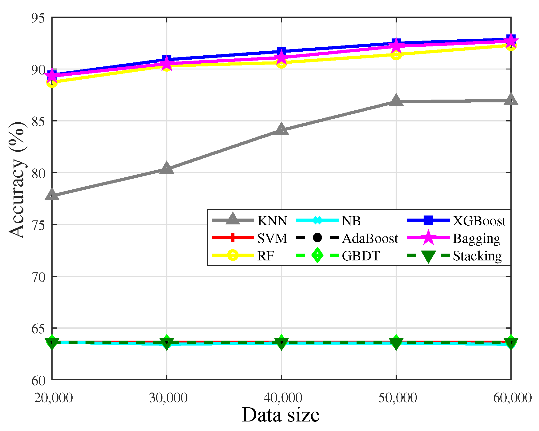
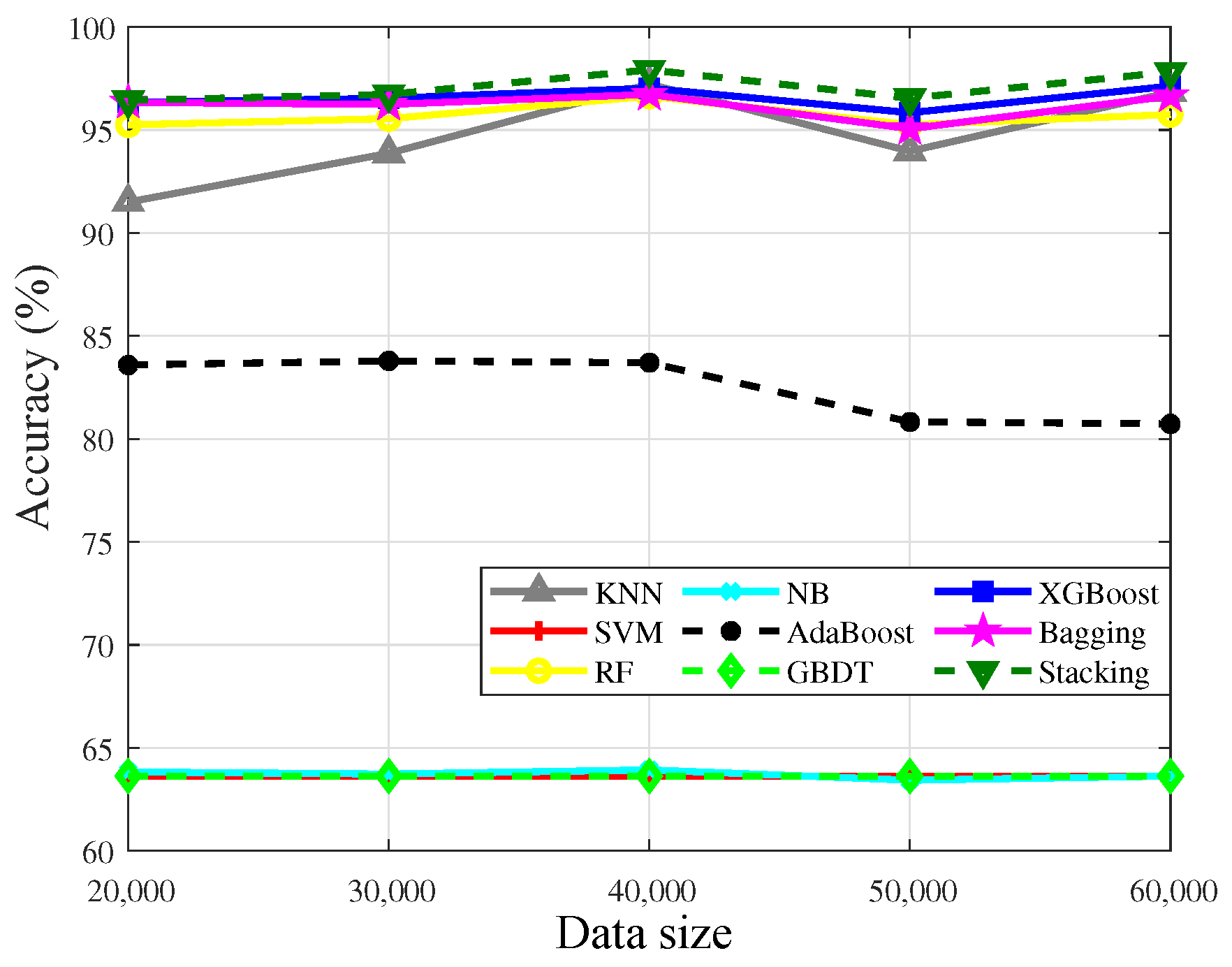
| Indicator | Accuracy | |||||||||||
|---|---|---|---|---|---|---|---|---|---|---|---|---|
| Size of Training Data | 20,000 | 30,000 | 40,000 | 50,000 | 60,000 | |||||||
| Proportion of Abnormal Data | 1% | 5% | 1% | 5% | 1% | 5% | 1% | 5% | 1% | 5% | ||
| Single model algorithms | kNN | 77.76 | 91.50 | 80.33 | 93.87 | 84.09 | 97.23 | 86.85 | 93.97 | 86.95 | 96.83 | |
| SVM | 63.63 | 63.63 | 63.63 | 63.63 | 63.63 | 63.63 | 63.63 | 63.63 | 63.63 | 63.63 | ||
| NB | 63.63 | 63.83 | 63.43 | 63.73 | 63.54 | 63.93 | 63.54 | 63.43 | 63.43 | 63.63 | ||
| Ensemble algorithms | RF | 88.73 | 95.25 | 90.31 | 95.55 | 90.61 | 96.64 | 91.40 | 95.25 | 92.29 | 95.75 | |
| Bagging | 89.32 | 96.34 | 90.51 | 96.24 | 91.10 | 96.73 | 92.19 | 95.06 | 92.68 | 96.65 | ||
| Boosting | AdaBoost | 63.63 | 83.59 | 63.63 | 83.79 | 63.63 | 83.70 | 63.63 | 80.83 | 63.63 | 80.73 | |
| GBDT | 63.63 | 63.63 | 63.63 | 63.63 | 63.63 | 63.63 | 63.63 | 63.63 | 63.63 | 63.63 | ||
| XGBoost | 89.42 | 96.34 | 90.90 | 96.54 | 91.69 | 97.03 | 92.49 | 95.84 | 92.88 | 97.13 | ||
| Stacking | 63.63 | 96.44 | 63.63 | 96.73 | 63.63 | 97.92 | 63.63 | 96.54 | 63.63 | 97.82 | ||
| Algorithms | Time Complexity | Order | Test |
|---|---|---|---|
| kNN | 1.49 s | ||
| SVM | 8.20 s | ||
| NB | 1.02 s | ||
| RF | 3.98 s | ||
| Bagging | 11.52 s | ||
| AdaBoost | 3.49 s | ||
| GBDT | 2.46 s | ||
| XGBoost | 1.79 s | ||
| Stacking | 47.78 s |
Disclaimer/Publisher’s Note: The statements, opinions and data contained in all publications are solely those of the individual author(s) and contributor(s) and not of MDPI and/or the editor(s). MDPI and/or the editor(s) disclaim responsibility for any injury to people or property resulting from any ideas, methods, instructions or products referred to in the content. |
© 2023 by the authors. Licensee MDPI, Basel, Switzerland. This article is an open access article distributed under the terms and conditions of the Creative Commons Attribution (CC BY) license (https://creativecommons.org/licenses/by/4.0/).
Share and Cite
Zhang, H.; Zhou, T.; Xu, T.; Hu, H. Remote Interference Discrimination Testbed Employing AI Ensemble Algorithms for 6G TDD Networks. Sensors 2023, 23, 2264. https://doi.org/10.3390/s23042264
Zhang H, Zhou T, Xu T, Hu H. Remote Interference Discrimination Testbed Employing AI Ensemble Algorithms for 6G TDD Networks. Sensors. 2023; 23(4):2264. https://doi.org/10.3390/s23042264
Chicago/Turabian StyleZhang, Hanzhong, Ting Zhou, Tianheng Xu, and Honglin Hu. 2023. "Remote Interference Discrimination Testbed Employing AI Ensemble Algorithms for 6G TDD Networks" Sensors 23, no. 4: 2264. https://doi.org/10.3390/s23042264