


Adversarial Auxiliary Weighted Subdomain Adaptation for Open-Set Deep Transfer Bridge Damage Diagnosis
Abstract
:1. Introduction
1.1. Related Work
1.2. Contributions
2. Preliminaries
2.1. Problem Formulate
2.2. Maximum Mean Discrepancy (MMD)
2.3. Convolutional Neural Network (CNN)
3. Proposed Method
3.1. Sub-Domain Adaptation Deep Transfer Learning Network
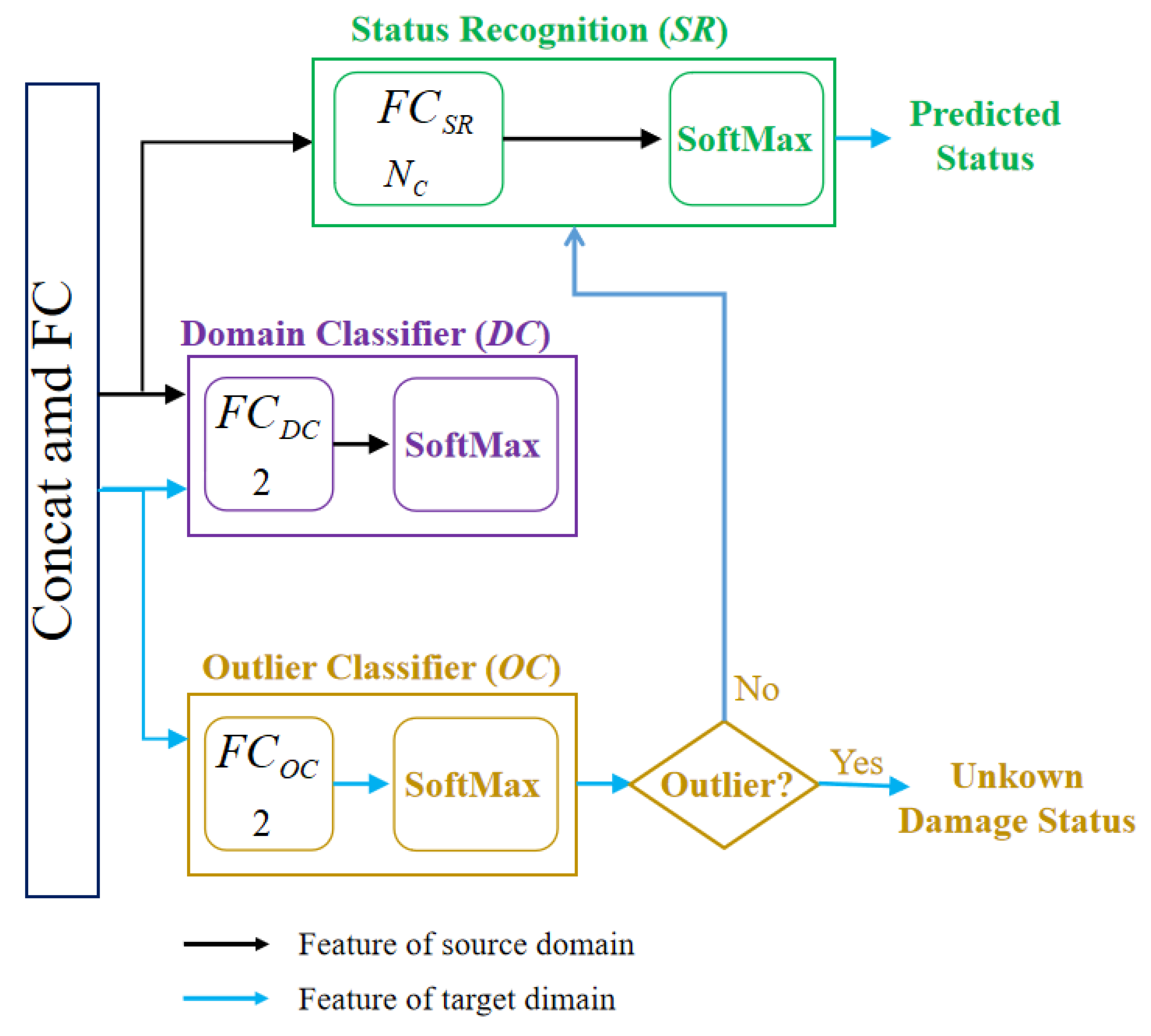
3.1.1. Status Recognition Module (SR)
3.1.2. Adversarial Learning Based Target Instance Weighting
3.1.3. Sub-Domain Adaptation with MCMK-WLMMD
3.1.4. Outlier Classifier
3.2. Optimization Objective
- (1)
- Minimizing the status recognition error in the source domain;
- (2)
- Maximizing the error of the domain classifier;
- (3)
- Minimizing the error of the sub-domain adaptation with MCMK-WLMMD;
- (4)
- Minimizing the error of the outlier classifier.
3.2.1. First Objective
3.2.2. Second Objective
3.2.3. Third Objective
3.2.4. Fourth Objective
3.3. Optimization Objective Training
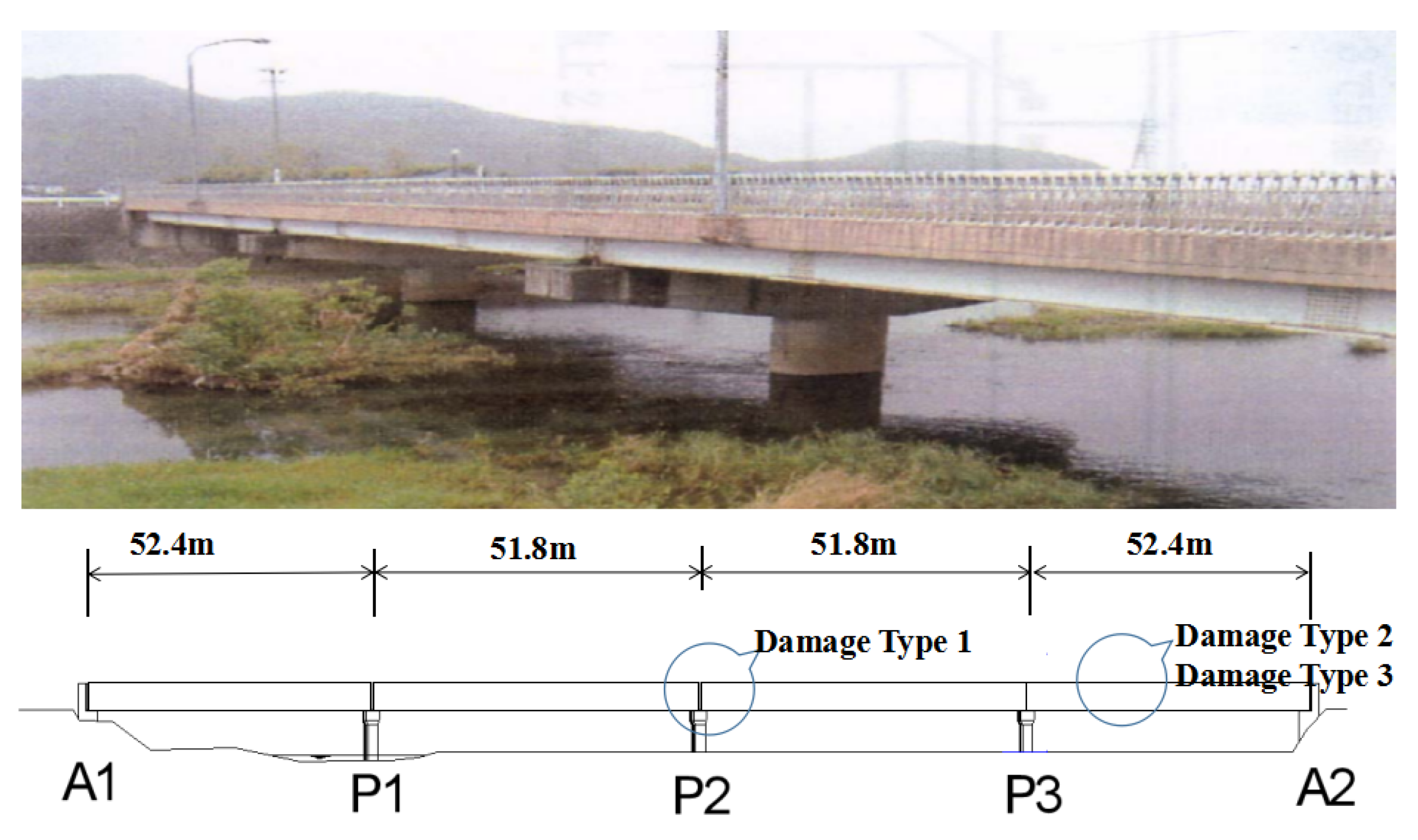
4. Field Bridge Experiment Result Study
4.1. Data Set
4.1.1. Data Set A
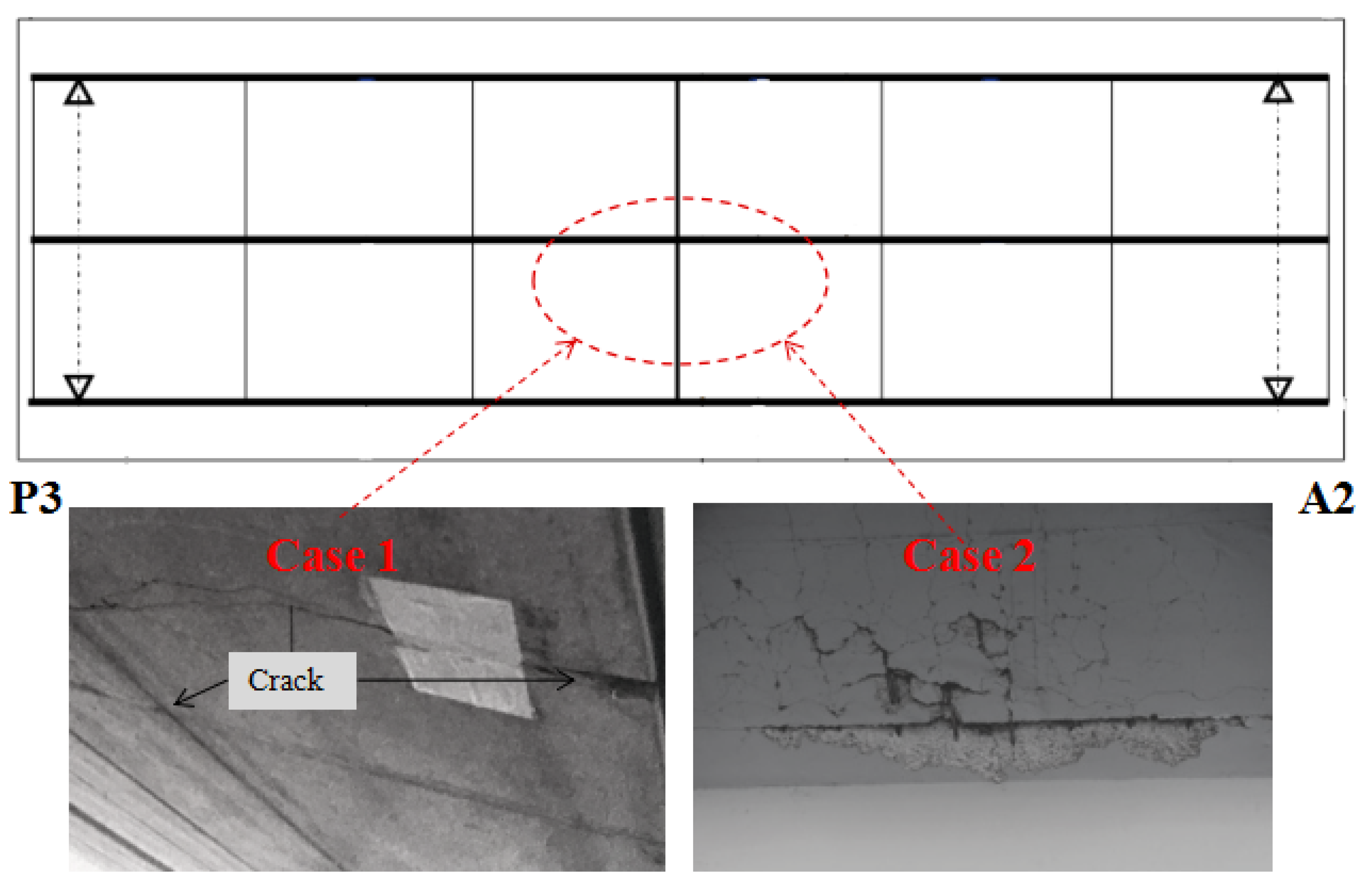
4.1.2. Data Set B
4.1.3. Data Set C
4.2. Pen-Set Transfer Tasks and Details
4.3. Methods for Comparison
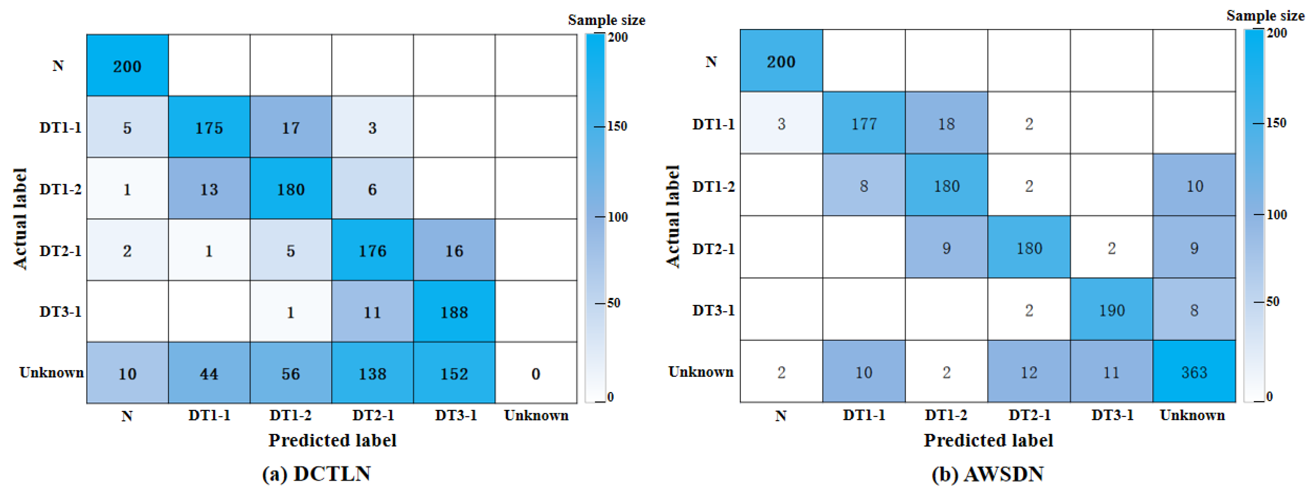
4.4. Result Analysis and Comparison
4.4.1. Cross-Bridge Damage Diagnosis Result Analysis
4.4.2. Visualization Analysis
5. Conclusions
Author Contributions
Funding
Conflicts of Interest
References
- An, Y.; Chatzi, E.; Sim, S.H.; Laflamme, S.; Blachowski, B. Recent progress and future trends on damage identification methods for bridge structures. Struct. Control Health Monit. 2019, 26, 1–30. [Google Scholar] [CrossRef]
- Azimi, M.; Eslamlou, A.D.; Pekcan, G. Data-Driven Structural Health Monitoring and Damage Detection through Deep Learning: State-of-the-Art Review. Sensors 2020, 20, 2778. [Google Scholar] [CrossRef] [PubMed]
- Vaez, S.R.H.; Arefzade, T. Vibration-based damage detection of concrete gravity dam monolith via wavelet transform. J. Vibro. Eng. 2017, 19, 204–213. [Google Scholar] [CrossRef] [Green Version]
- Cha, Y.-J.; Choi, W.; Büyüköztürk, O. Deep learning-based crack damage detection using convolutional neural networks. Comput. Aided Civ. Infrastruct. Eng. 2017, 32, 361–378. [Google Scholar] [CrossRef]
- Lin, Y.-Z.; Nie, Z.-H.; Ma, H.-W. Structural damage detection with automatic feature-extraction through deep learning. Comput. Aided Civ. Infrastruct. Eng. 2017, 32, 1025–1046. [Google Scholar] [CrossRef]
- Li, X.; Lin, Y.; Ma, H.; Nie, Z. Plication of bridge damage identification based on convolutional neural network. J. Qinghai Univ. 2018, 36, 1–6. [Google Scholar]
- Li, X.S.; Ma, H.W.; Lin, Y.Z. Structural damage identification based on convolution neural network. J. Vib. Shock. 2019, 38, 159–167. [Google Scholar]
- Abdeljaber, O.; Avci, O.; Kiranyaz, M.S.; Boashash, B.; Sodano, H.; Inman, D.J. 1-D CNNs for structural damage detection: Verification on a structural health monitoring benchmark data. Neuro Comput. 2018, 275, 1308–1317. [Google Scholar] [CrossRef]
- Zhang, Y.; Miyamori, Y.; Mikami, S.; Saito, T. Vibration-based structural state identification by a 1-dimensional convolutional neural network. Comput. Aided Civ. Infrastruct. Eng. 2019, 34, 15–19. [Google Scholar] [CrossRef]
- Liu, H.; Zhang, Y. Image-driven structural steel damage condition assessment method using deep learning algorithm. Measurement 2019, 133, 168–181. [Google Scholar] [CrossRef]
- Tang, Z.; Chen, Z.; Bao, Y.; Li, H. Convolutional neural network-based data anomaly detection method using multiple information for structural health monitoring. Struct. Control Monit. 2019, 26, e2296. [Google Scholar] [CrossRef] [Green Version]
- Weiss, K.; Khoshgoftaar, T.M.; Wang, D.D. A survey of transfer learning. J. Big Data 2016, 3, 1–40. [Google Scholar] [CrossRef]
- Pan, S.J.; Yang, Q. A survey on transfer learning. IEEE Trans. Knowl. Data Eng. 2010, 22, 1345–1359. [Google Scholar] [CrossRef]
- Ben-David, S.; Blitzer, J.; Crammer, K.; Kulesza, A.; Pereira, F.; Vaughan, J.W. A theory of learning from different domains. J. Mach. Learn. 2010, 79, 151–175. [Google Scholar] [CrossRef] [Green Version]
- Zhuang, F.; Ping, L.; Qing, H.; Shi, Z. Survey on transfer learning research. J. Softw. 2015, 26, 26–39. [Google Scholar]
- Zhang, R.; Tao, H.; Wu, L.; Guan, Y. Transfer learning with neural networks for bearing fault diagnosis in changing working conditions. IEEE Access 2017, 5, 14347–14357. [Google Scholar] [CrossRef]
- Han, D.; Liu, Q.; Fan, W. A new image classification method using CNN transfer learning and web data augmentation. Expert Syst. Appl. 2018, 95, 43–56. [Google Scholar] [CrossRef]
- Chen, D.M.; Yang, S.; Zhou, F. Incipient fault diagnosis based on DNN with transfer learning. In Proceedings of the International Conference on Control, Automation and Information Sciences, Hangzhou, China, 24–27 October 2018. [Google Scholar]
- Wang, X.; Schneider, J. Flexible transfer learning under support and model shift. Adv. Neural Inf. Process. Syst. 2014, 27, 1898–1906. [Google Scholar]
- Li, X.; Zhang, W. Deep learning-based partial domain adaptation method on intelligent machinery fault diagnostics. IEEE Trans. Ind. Electron. 2021, 68, 4351–4361. [Google Scholar] [CrossRef]
- Chen, Z.; Gryllias, K.; Li, W. Intelligent fault diagnosis for rotary machinery using transferable convolutional neural network. J. IEEE Trans. Ind. Inform. 2019, 16, 339–349. [Google Scholar] [CrossRef]
- Tzeng, E.; Hoffman, J.; Saenko, K. Adversarial discriminative domain adaptation. In Proceedings of the IEEE Conference on Computer Vision and Pattern Recognition, Honolulu, HI, USA, 21–26 July 2017; pp. 2962–2971. [Google Scholar]
- Long, M.; Cao, Z.; Wang, J. Conditional adversarial domain adaptation. Proc. Adv. Neural Inf. Process. Syst. 2018, 31, 1640–1650. [Google Scholar]
- Chen, Z.; He, G.; Li, J.; Liao, Y. Domain adversarial transfer network for cross-domain fault diagnosis of rotary machinery. IEEE Trans. Instrum. Meas. 2020, 69, 8702–8712. [Google Scholar] [CrossRef]
- Li, T.; Zhao, Z.; Sun, C.; Yan, R. Domain adversarial graph convolutional network for fault diagnosis under variable working conditions. IEEE Trans. Instrum. Meas. 2021, 70, 3515010. [Google Scholar] [CrossRef]
- Lu, W.; Liang, B.; Cheng, Y.; Meng, D.; Yang, J.; Zhang, T. Deep model based domain adaptation for fault diagnosis. IEEE Trans. Ind. Electron. 2016, 388, 2296–2305. [Google Scholar] [CrossRef]
- Wen, L.; Gao, L.; Li, X. A new deep transfer learning based on sparse auto-encoder for fault diagnosis. IEEE Trans. Syst. Man Cybern. Syst. 2019, 49, 136–144. [Google Scholar] [CrossRef]
- Lu, N.; Xiao, H.; Sun, Y. A new method for intelligent fault diagnosis of machines based on unsupervised domain adaptation. Neurocomputing 2021, 427, 96–109. [Google Scholar] [CrossRef]
- Yang, B.; Lei, Y.; Jia, F. A polynomial kernel induced distance metric to improve deep transfer learning for fault diagnosis of machines. IEEE Trans. Ind. Electron. 2020, 67, 9747–9757. [Google Scholar] [CrossRef]
- Cao, X.; Wang, Y.; Chen, B. Domain-adaptive intelligence for fault diagnosis based on deep transfer learning from scientific test rigs to industrial applications. Neural Comput. 2021, 4483–4499. [Google Scholar] [CrossRef]
- Zhu, J.; Chen, N.; Shen, C. New deep transfer learning method for bearing fault diagnosis under different working conditions. IEEE Sens. J. 2020, 8394–8402. [Google Scholar] [CrossRef]
- Che, C.; Wang, H.; Ni, X. Domain adaptive deep belief network for rolling bearing fault diagnosis. Comput. Ind. Eng. 2020, 143, 106427. [Google Scholar] [CrossRef]
- Han, T.; Liu, C.; Yang, W.; Jiang, D. Deep transfer network with joint distribution adaptation: A new intelligent fault diagnosis framework for industry application. ISA Trans. 2020, 269–281. [Google Scholar] [CrossRef] [PubMed] [Green Version]
- Qian, W.; Li, S.; Yi, P. A novel transfer learning method for robust fault diagnosis of rotating machines under variable working conditions. Measurement 2019, 138, 514–525. [Google Scholar] [CrossRef]
- Cao, X.; Chen, B.; Zeng, N. A deep domain adaption model with multi-task networks for planetary gearbox fault diagnosis. Neurocomputing 2020, 409, 173–190. [Google Scholar] [CrossRef]
- Ding, Z.; Fu, Y. Robust transfer metric learning for image classification. IEEE Trans. Image Process. 2017, 26, 660–670. [Google Scholar] [CrossRef] [PubMed]
- Gao, Y.; Mosalam, K.M. Deep Transfer Learning for Image-Based Structural Damage Recognition. Comput. Aided Civ. Infrastruct. Eng. 2018, 33, 748–768. [Google Scholar] [CrossRef]
- Zhang, K.; Cheng, H.D.; Zhang, B. Unified Approach to Pavement Crack and Sealed Crack Detection Using Preclassification Based on Transfer Learning. J. Comput. Civ. Eng. 2018, 32, 04018001. [Google Scholar] [CrossRef]
- Gopalakrishnan, K.; Khaitan, S.K.; Choudhary, A.; Agrawal, A. Deep Convolutional Neural Networks with transfer learning for computer vision-based data-driven pavement distress detection. Constr. Build. Mater. 2017, 157, 322–330. [Google Scholar] [CrossRef]
- Perez, H.; Tah, J.H.M.; Mosavi, A. Deep Learning for Detecting Building Defects Using Convolutional Neural Networks. Sensors 2019, 19, 3556. [Google Scholar] [CrossRef] [Green Version]
- Liu, H.; Cao, Z.; Long, M. Separate to adapt: Open set domain adaptation via progressive separation. In Proceedings of the IEEE/CVF Conference on Computer Vision and Pattern Recognition, Long Beach, CA, USA, 15–20 June 2019; pp. 2927–2936. [Google Scholar]
- Fang, Z.; Lu, J.; Liu, F. Open set domain adaptation: Theoretical bound and algorithm. IEEE Trans. Neural Netw. Learn. Syst. 2019, 32, 361–378. [Google Scholar] [CrossRef]
- Busto, P.; Gall, J. Open set domain adaptation. IEEE Int. Conf. Comput. Vis. 2017, 18, 754–763. [Google Scholar]
- Zhu, Y.; Zhuang, F.; Wang, J.; Ke, G.; Chen, J.; Bian, J.; Xiong, H.; He, Q. Deep Subdomain Adaptation Network for Image Classification. IEEE Trans. Neural Netw. Learn. Syst. 2021, 32, 1713–1722. [Google Scholar] [CrossRef] [PubMed]
- Jain, L.; Scheirer, W. Multi-class open set recognition using probability of inclusion. In Proceedings of the European Conference on Computer Vision, Zurich, Switzerland, 6–12 September 2014; pp. 393–409. [Google Scholar]
- Tzeng, E.; Hoffman, J.; Zhang, N.; Saenko, K. Deep domain confusion: Maximizing for domain invariance. arXiv 2014, arXiv:1412.3474. [Google Scholar]
- Guo, L.; Lei, Y.; Xing, S.; Yan, T.; Li, N. Deep convolutional transfer learning network: A new method for intelligent fault diagnosis of machines with unlabeled data. IEEE Trans. Ind. Electron. 2019, 66, 7316–7325. [Google Scholar] [CrossRef]


| No. | Layer | Function | Parameters |
|---|---|---|---|
| 1 | Input | L | |
| 2 | 1st Convolution | ||
| 3 | Pooling | k | |
| 4 | 2nd Convolution | ||
| 5 | Pooling | k | |
| 6 | 3rd Convolution | ||
| 7 | Pooling | k | |
| 8 | 4th Convolution | ||
| 9 | Pooling | k | |
| 10 | 5th Convolution | ||
| 11 | Pooling | k | |
| 12 | MPME | Multi-channel Parallel Multi-scale Extractor | / |
| 13 | FC | Concat and Flatten | / |
| 14 | Softmax | / |
| Damage Mode | Type | Degree | Load |
|---|---|---|---|
| N | No damage | No damage | 20 kmph, car |
| Type I | case 1 | 20 kmph, car | |
| Type I | case 2 | 20 kmph, car | |
| Type II | case 1 | 20 kmph, car | |
| Type II | case 2 | 20 kmph, car | |
| Type III | case 1 | 20 kmph, car | |
| Type III | case 2 | 20 kmph, car |
| Condition | Unit | Degree (Percent) |
|---|---|---|
| N | No damage | No damage |
| Reduce the intensity of the portion near A2 in unit 6 | 10 | |
| Reduce the intensity of the portion near A2 in unit 6 | 20 | |
| 12 | 5 | |
| 12 | 15 | |
| 16, 17, 18 | 15, 35, 5 | |
| 16, 17, 18 | 15, 65, 5 |
| Mode | Type | Load |
|---|---|---|
| N | No damage | 40 kmph, car |
| Bearing corrosion: case 1 | 40 kmph, car | |
| Bearing corrosion: case 2 | 40 kmph, car | |
| Steel frame corrosion: case 1 | 40 kmph, car | |
| Steel frame corrosion: case 2 | 40 kmph, car | |
| Concrete deck deterioration: case 1 | 40 kmph, car | |
| Concrete deck deterioration: case 2 | 40 kmph, car |
| Transfer Tasks | Source States | Training Data-Set | Testing Data-Set |
|---|---|---|---|
| all | 100% Labeled data-set A and 50% unlabeled data-set B | 50% unlabeled data-set B | |
| 100% Labeled data-set A and 50% unlabeled data-set B | 50% unlabeled data-set B | ||
| 100% Labeled data-set A and 50% unlabeled data-set C | 50% unlabeled data-set C | ||
| 100% Labeled data-set A and 50% unlabeled data-set C | 50% unlabeled data-set C | ||
| 100% Labeled data-set B and 50% unlabeled data-set C | 50% unlabeled data-set C | ||
| 100% Labeled data-set B and 50% unlabeled data-set C | 50% unlabeled data-set C | ||
| 100% Labeled data-set B and 50% unlabeled data-set A | 50% unlabeled data-set A | ||
| 100% Labeled data-set C and 50% unlabeled data-set A | 50% unlabeled data-set A | ||
| 100% Labeled data-set C and 50% unlabeled data-set B | 50% unlabeled data-set B |
| Method No. | Method Name | Feature | Transfer Leaning Type |
|---|---|---|---|
| M1 | CNN | Learned feature | No transfer |
| M2 | OSVM | Learned feature | No transfer |
| M3 | OSVM-MMD | Learned feature | MMD with OSVM |
| M4 | DDC | Learned feature | MMD |
| M5 | DCTLN | Learned feature | MMD with adversarial learning |
| M6 | AWSDN | Learned feature | MCMK-WLMMD and adversarial auxiliary weighting |
| Condition | Precision (%) | Recall | Sample |
|---|---|---|---|
| N | 98.52 | 1.00 | 200 |
| 92.75 | 0.92 | 200 | |
| 90.12 | 0.91 | 200 | |
| 92.91 | 0.92 | 200 | |
| 95.65 | 0.97 | 200 | |
| 95.08 | 0.93 | 400 | |
| Average | 94.17 | 0.94 |
Disclaimer/Publisher’s Note: The statements, opinions and data contained in all publications are solely those of the individual author(s) and contributor(s) and not of MDPI and/or the editor(s). MDPI and/or the editor(s) disclaim responsibility for any injury to people or property resulting from any ideas, methods, instructions or products referred to in the content. |
© 2023 by the authors. Licensee MDPI, Basel, Switzerland. This article is an open access article distributed under the terms and conditions of the Creative Commons Attribution (CC BY) license (https://creativecommons.org/licenses/by/4.0/).
Share and Cite
Xiao, H.; Dong, L.; Wang, W.; Ogai, H. Adversarial Auxiliary Weighted Subdomain Adaptation for Open-Set Deep Transfer Bridge Damage Diagnosis. Sensors 2023, 23, 2200. https://doi.org/10.3390/s23042200
Xiao H, Dong L, Wang W, Ogai H. Adversarial Auxiliary Weighted Subdomain Adaptation for Open-Set Deep Transfer Bridge Damage Diagnosis. Sensors. 2023; 23(4):2200. https://doi.org/10.3390/s23042200
Chicago/Turabian StyleXiao, Haitao, Limeng Dong, Wenjie Wang, and Harutoshi Ogai. 2023. "Adversarial Auxiliary Weighted Subdomain Adaptation for Open-Set Deep Transfer Bridge Damage Diagnosis" Sensors 23, no. 4: 2200. https://doi.org/10.3390/s23042200