Author Contributions
Conceptualization, T.C.; methodology, T.C. and F.S.; titration software, E.V.; validation, T.C.; formal analysis, T.C. and F.S.; investigation, T.C.; resources, T.C. and F.S.; data curation, T.C. and E.V.; writing—original draft preparation, T.C.; writing—review and editing, T.C. and E.V.; supervision, T.C.; project administration, T.C.; funding acquisition, T.C. All authors have read and agreed to the published version of the manuscript.
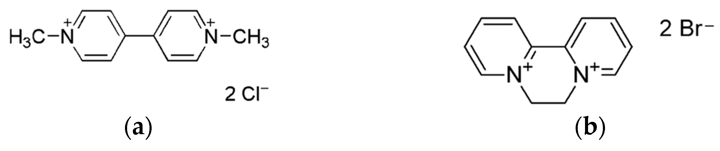
Figure 1.
(a) Paraquat dichloride, PQ. (b) Diquat dibromide, DQ.
Figure 1.
(a) Paraquat dichloride, PQ. (b) Diquat dibromide, DQ.
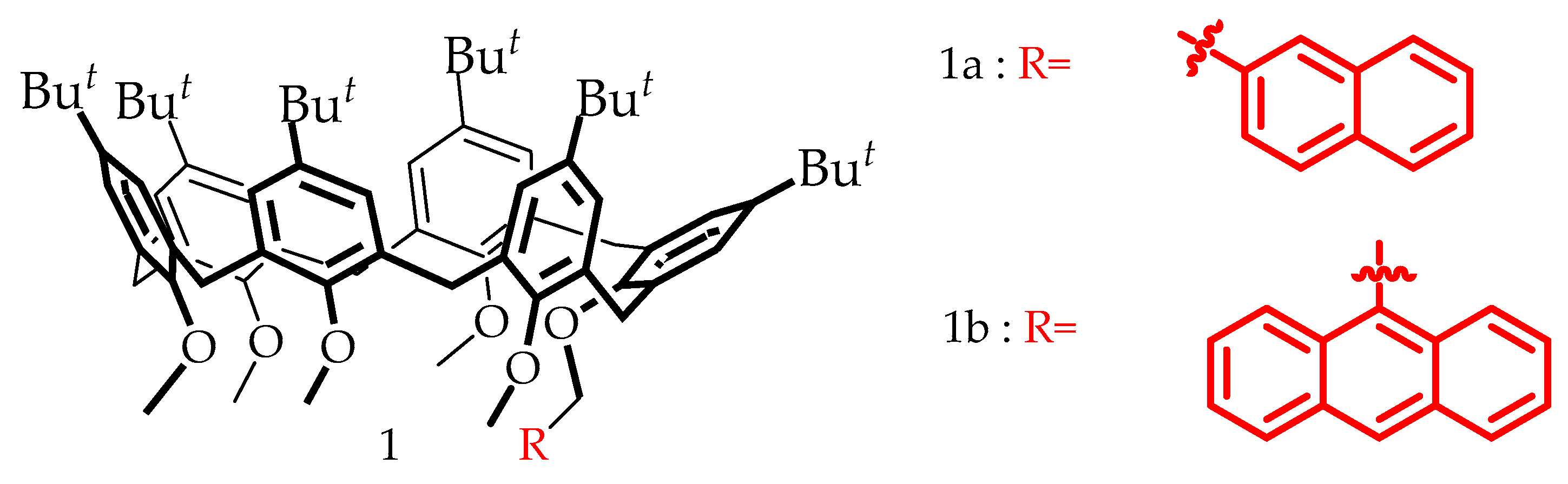
Figure 2.
Calix[6]arene hosts 1a and 1b with fluorophores covalently linked.
Figure 2.
Calix[6]arene hosts 1a and 1b with fluorophores covalently linked.
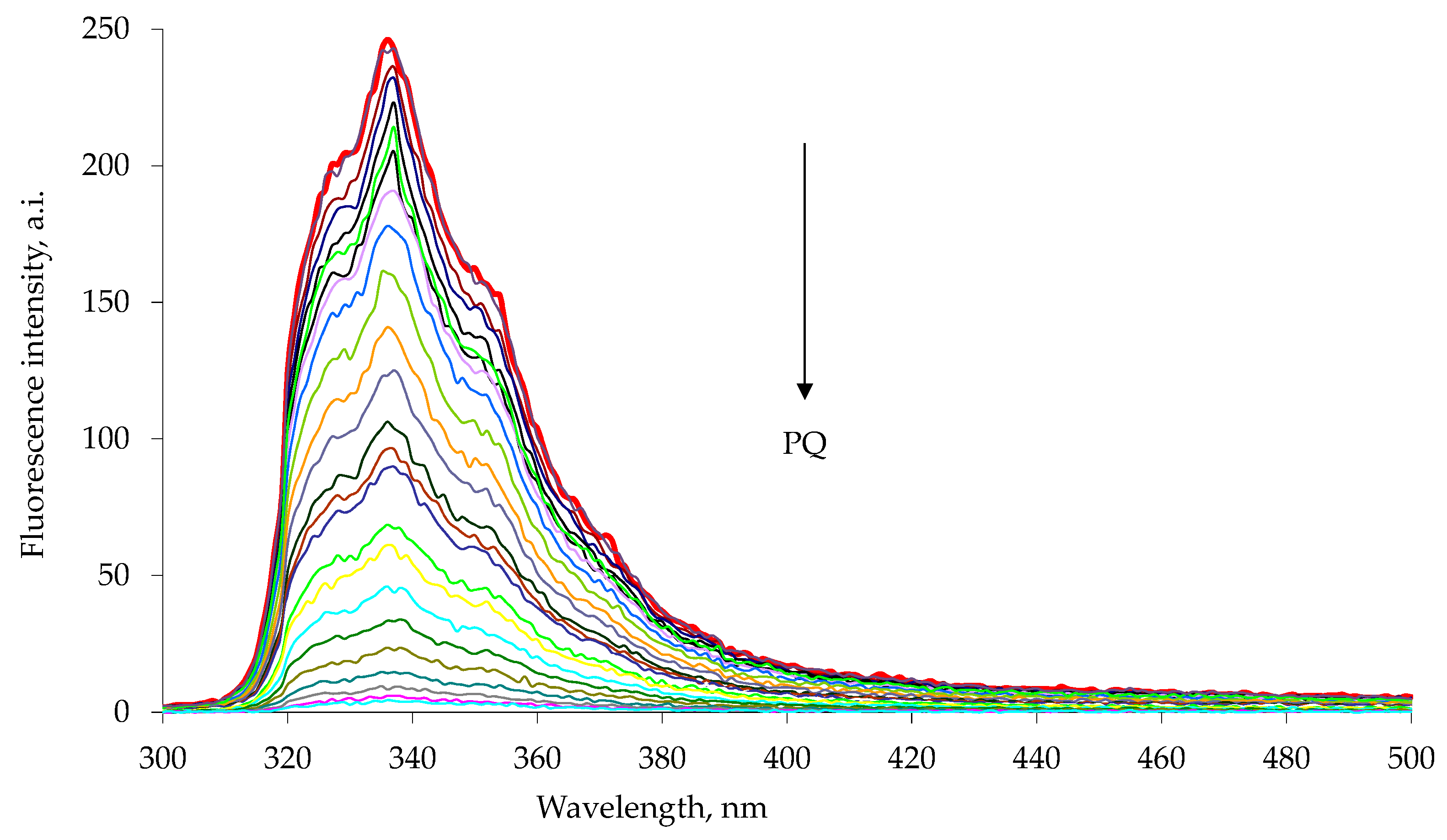
Figure 3.
Fluorescence quenching of 1a host with increasing paraquat concentration, PQ, in chloroform–methanol 1:1 solution at 25 °C. The experimental data are reported in
Table 1. The emission spectra were measured with excitation at 285 nm. Each spectrum is reported with different color line (Entry 1–25
Table 1).
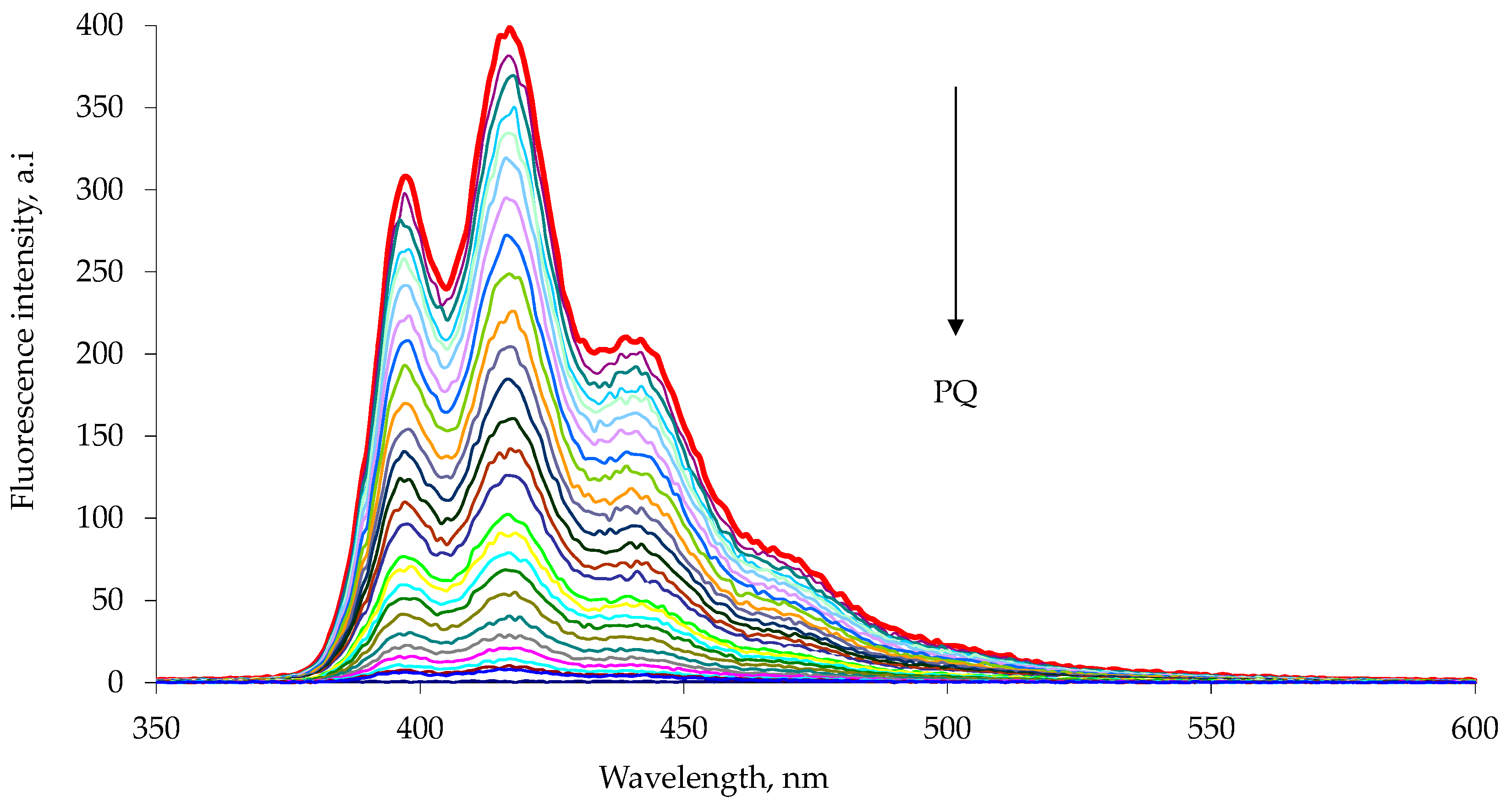
Figure 4.
Fluorescence quenching of 1b host with increasing paraquat concentration, PQ, in chloroform–methanol 1:1 solution at 25 °C. The experimental data are reported in
Table 2. The emission spectra were measured with excitation at 263 nm. Each spectrum is reported with different color line (Entry 1–25
Table 2).
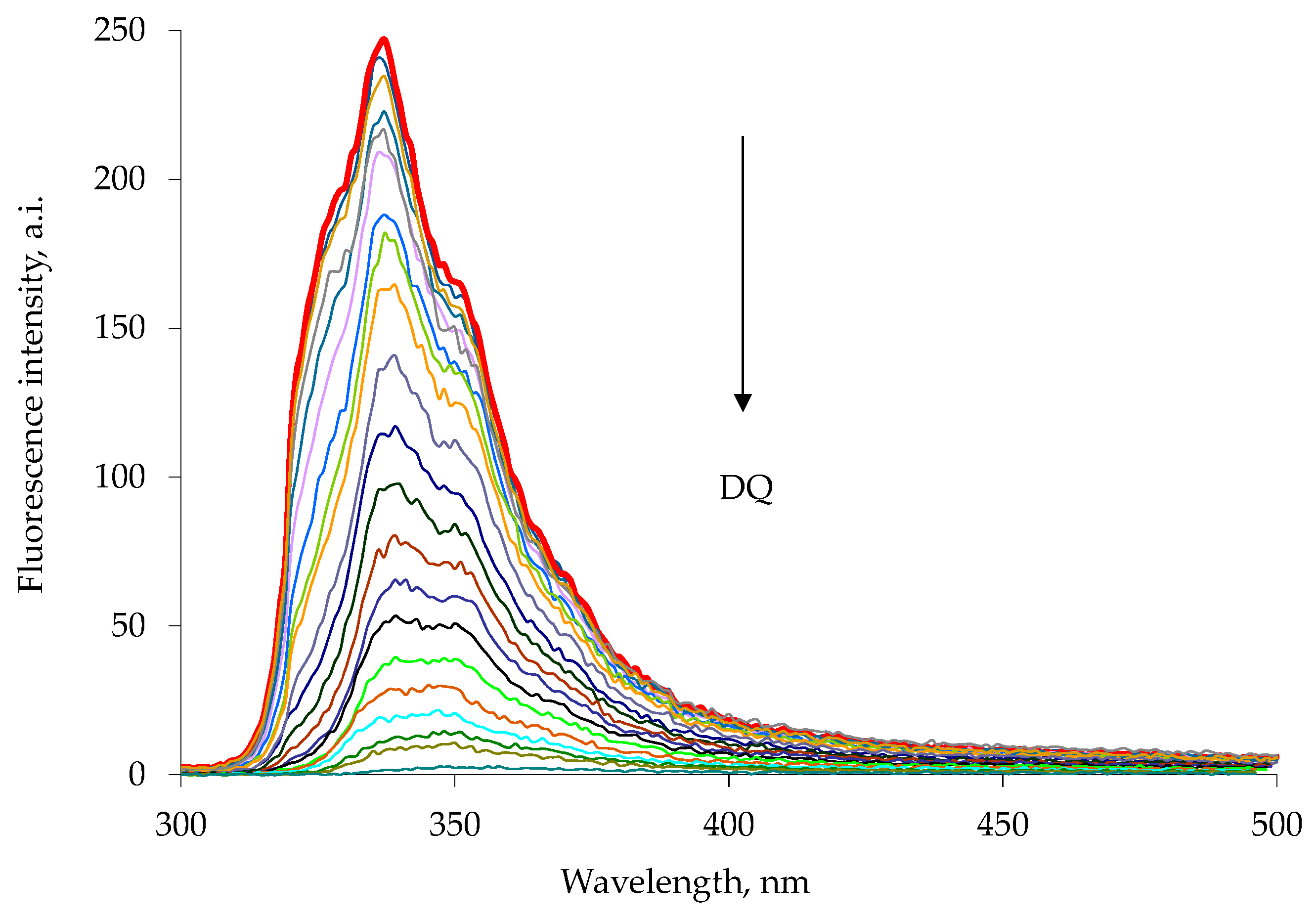
Figure 5.
Fluorescence quenching of 1a host with increasing diquat concentration, DQ, in chloroform–methanol 1:1 solution at 25 °C. The emission spectra were measured with excitation at 285 nm. Each spectrum is reported with different color line (Entry 1–18
Table 3).
Figure 5.
Fluorescence quenching of 1a host with increasing diquat concentration, DQ, in chloroform–methanol 1:1 solution at 25 °C. The emission spectra were measured with excitation at 285 nm. Each spectrum is reported with different color line (Entry 1–18
Table 3).
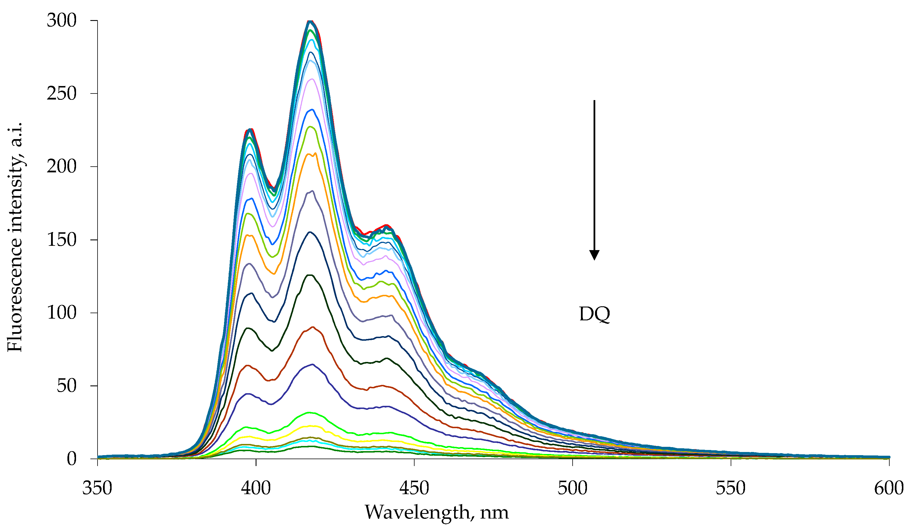
Figure 6.
Fluorescence quenching of 1b host with increasing diquat concentration in chloroform–methanol 1:1 solution at 25 °C. The emission spectra were measured with excitation at 263 nm. Each spectrum is reported with different color line (Entry 1–20
Table 4).
Figure 6.
Fluorescence quenching of 1b host with increasing diquat concentration in chloroform–methanol 1:1 solution at 25 °C. The emission spectra were measured with excitation at 263 nm. Each spectrum is reported with different color line (Entry 1–20
Table 4).
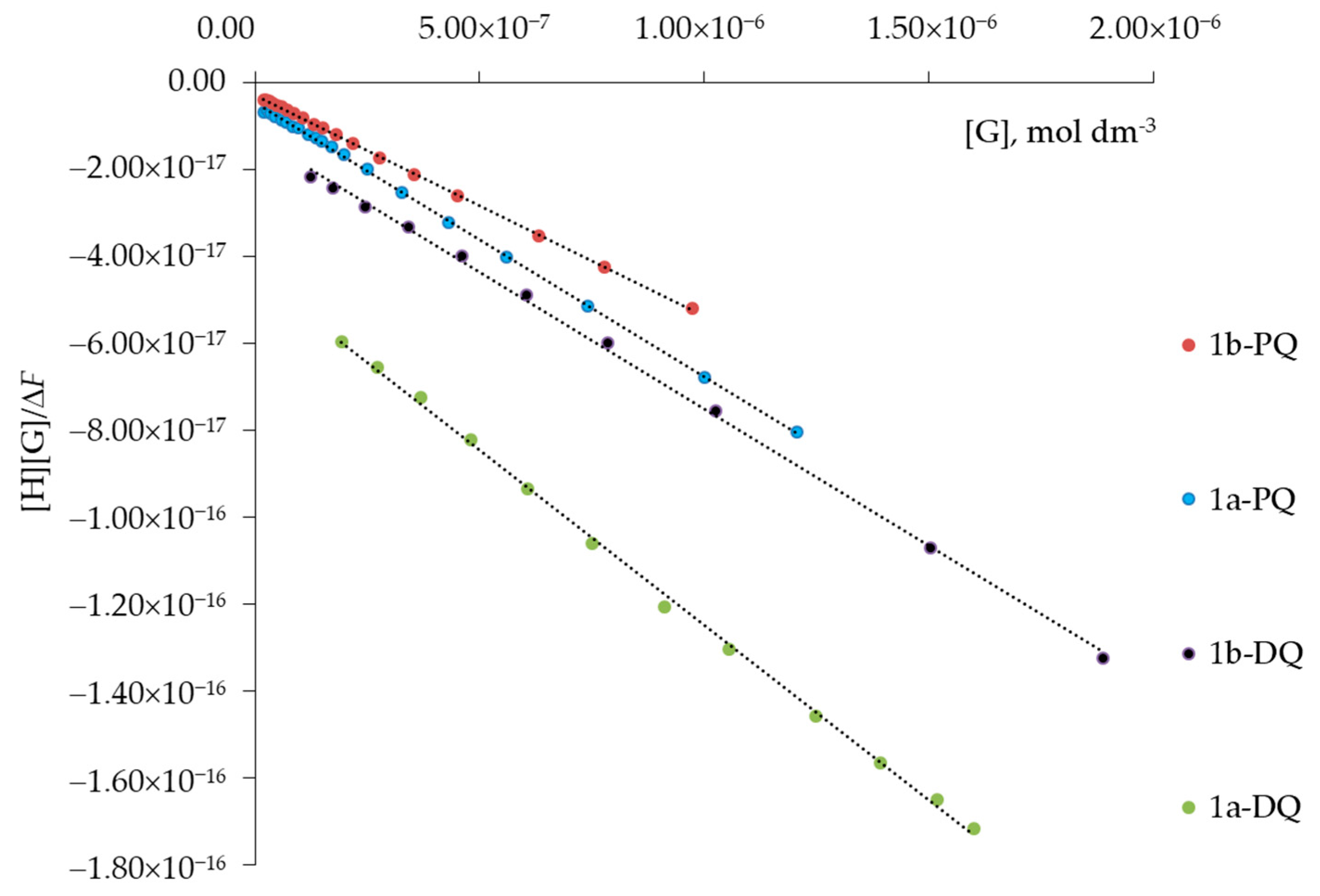
Figure 7.
Typical plot of [H][G]/ΔF versus [G], mol dm−3 for the complexation of host 1a (or 1b) with the guest (G), paraquat (PQ) or diquat (DQ). The dashed lines represent the fitted function by using Equation (1).
Figure 7.
Typical plot of [H][G]/ΔF versus [G], mol dm−3 for the complexation of host 1a (or 1b) with the guest (G), paraquat (PQ) or diquat (DQ). The dashed lines represent the fitted function by using Equation (1).
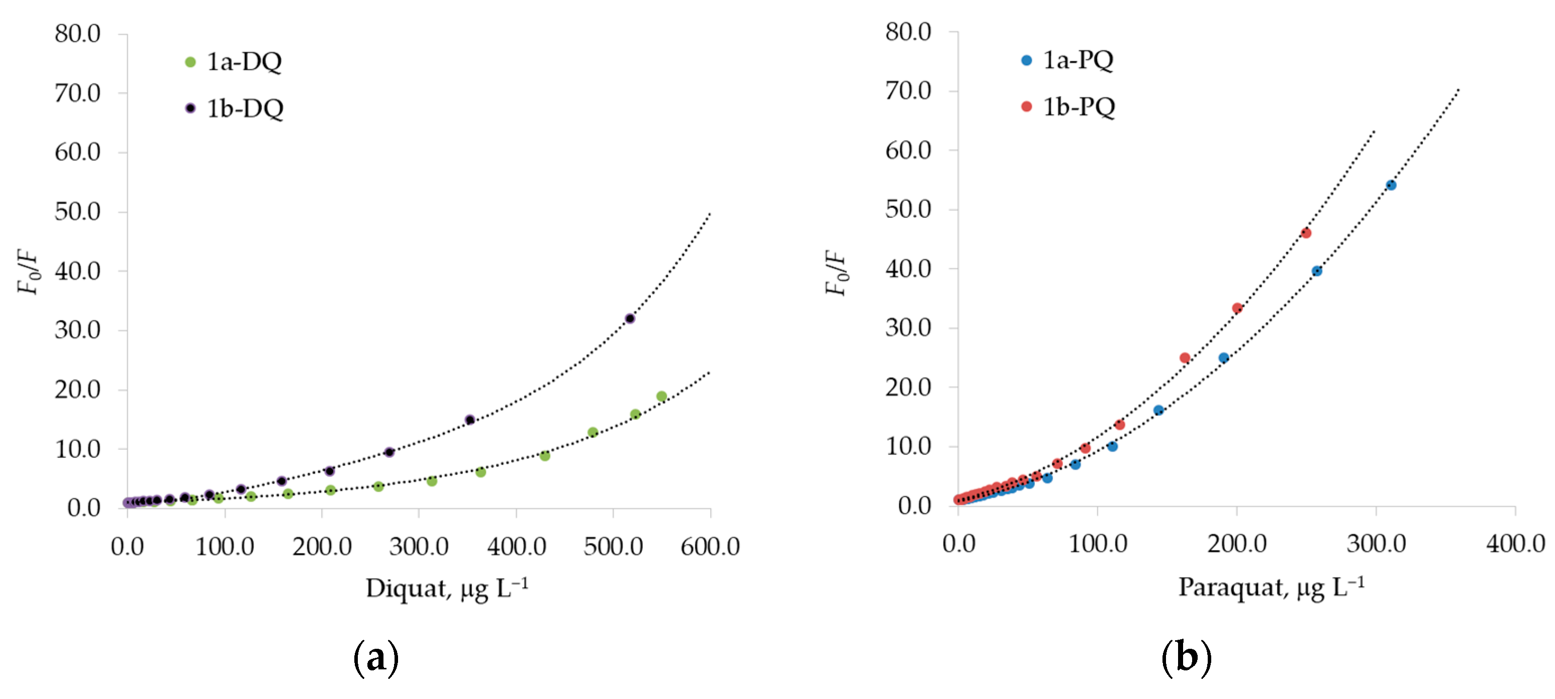
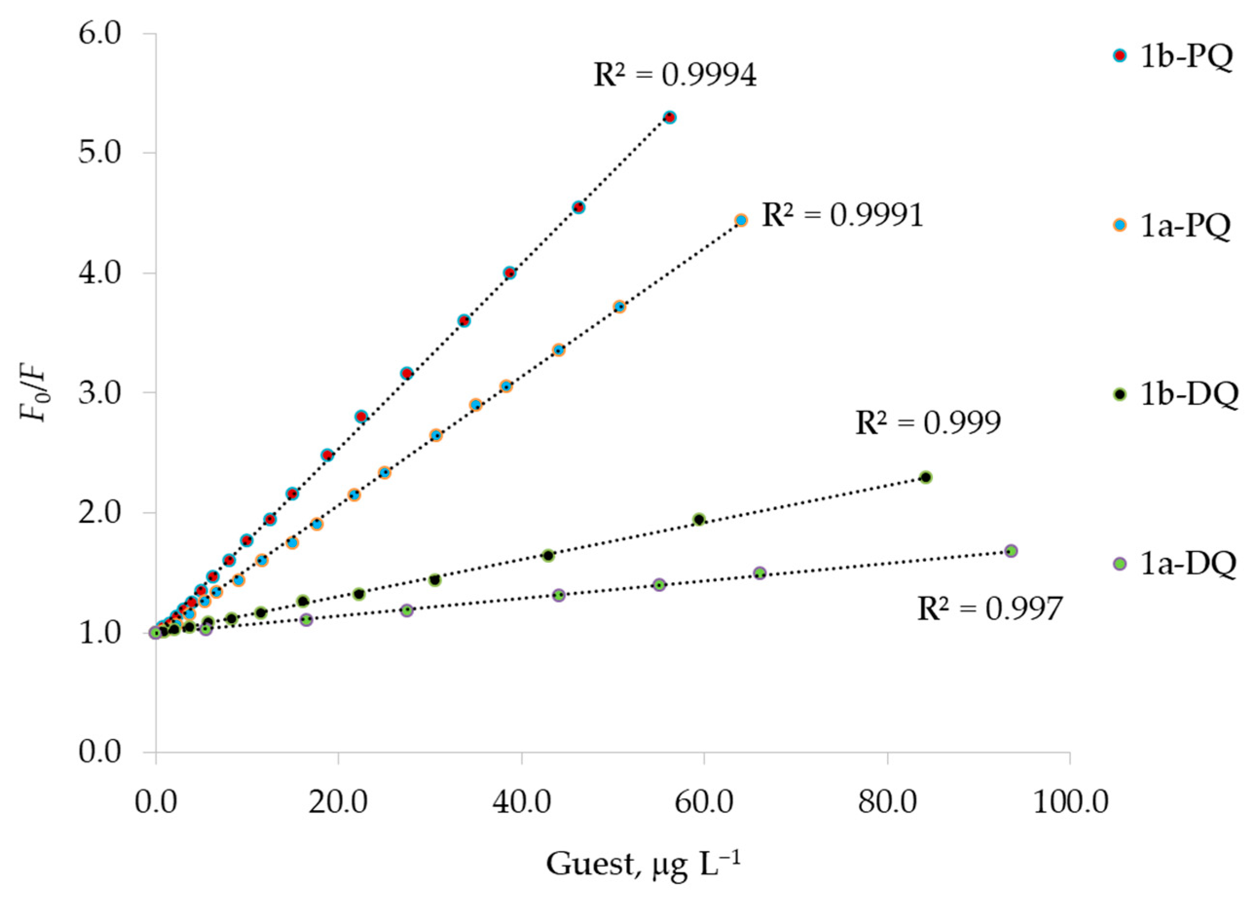
Figure 8.
A modified Stern–Volmer plot of F0/F against increasing concentration of quencher guests. (a) The experimental behavior for the diquat, DQ, as quencher of 1a and 1b fluorophores. (b) The experimental behavior for the paraquat, PQ, as quencher of 1a and 1b fluorophores. The dashed lines represent the curvature provided by Equation (4). The excitation wavelength was set to 285 nm and 263 nm, and the fluorescence value F was measured at 336 nm and 416 nm for the fluorophores 1a and 1b, respectively. F0 is the fluorescence intensity in the absence of quencher PQ or DQ.
Figure 9.
Stern–Volmer plots for the fluorescence quenching of 1a and 1b host with paraquat, PQ, and diquat, DQ, as guests. The excitation wavelength was set to 285 nm and 263 nm, and the fluorescence value F was measured at 336 nm and 416 nm for the fluorophores 1a and 1b, respectively. F0 is the fluorescence intensity in the absence of quencher PQ or DQ at 336 nm or 416 nm.
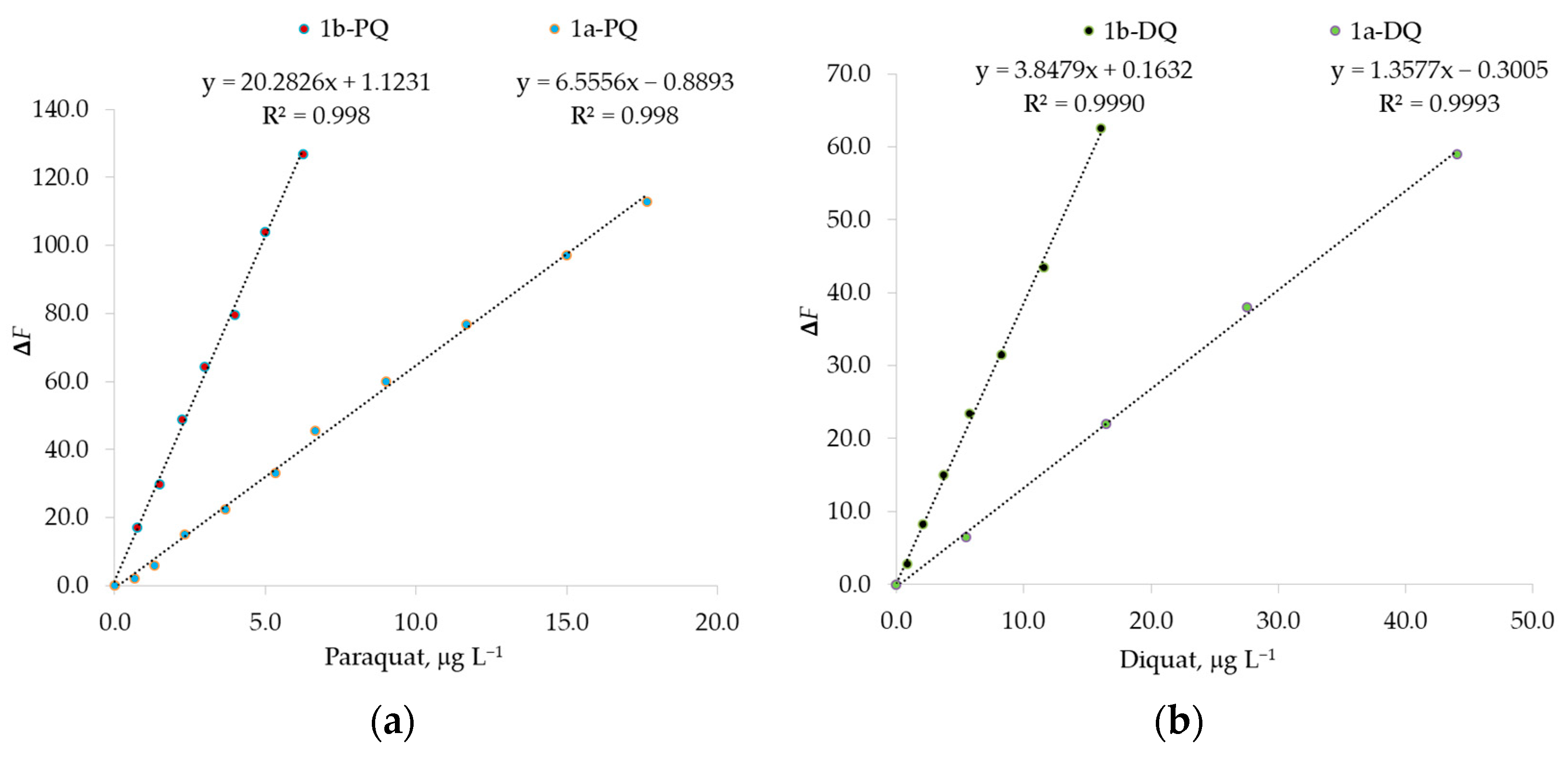
Figure 10.
Fluorescence change ΔF = F0 − F of fluorophores 1a and 1b against (a) paraquat, PQ, or (b) diquat, DQ, concentrations in chloroform–methanol solution 1:1. F0 indicates the fluorescence at [PQ] = 0 μg L−1 or [DQ] = 0 μg L−1 at 336 nm for naphthalene fluorophore 1a and at 416 nm for anthracene fluorophore 1b.
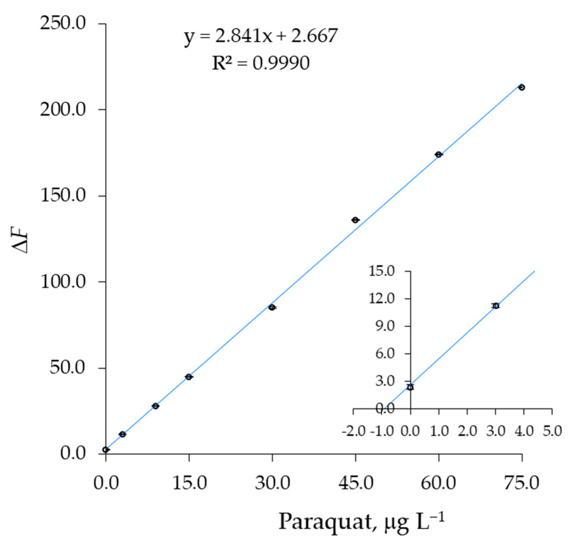
Figure 11.
Standard additions plot obtained by adding a methanol solution of paraquat, PQ, and 1b to a tap water sample (3 replicates). The sample was divided into 8 equal aliquots. The spike concentration of 1.0 μg L−1 was normalized to the total volume of solvent, 60/40 methanol/water. Inset: The straight line intersects the x-axis to the expected concentration of (1.1 ± 0.1) μg L−1 of PQ.
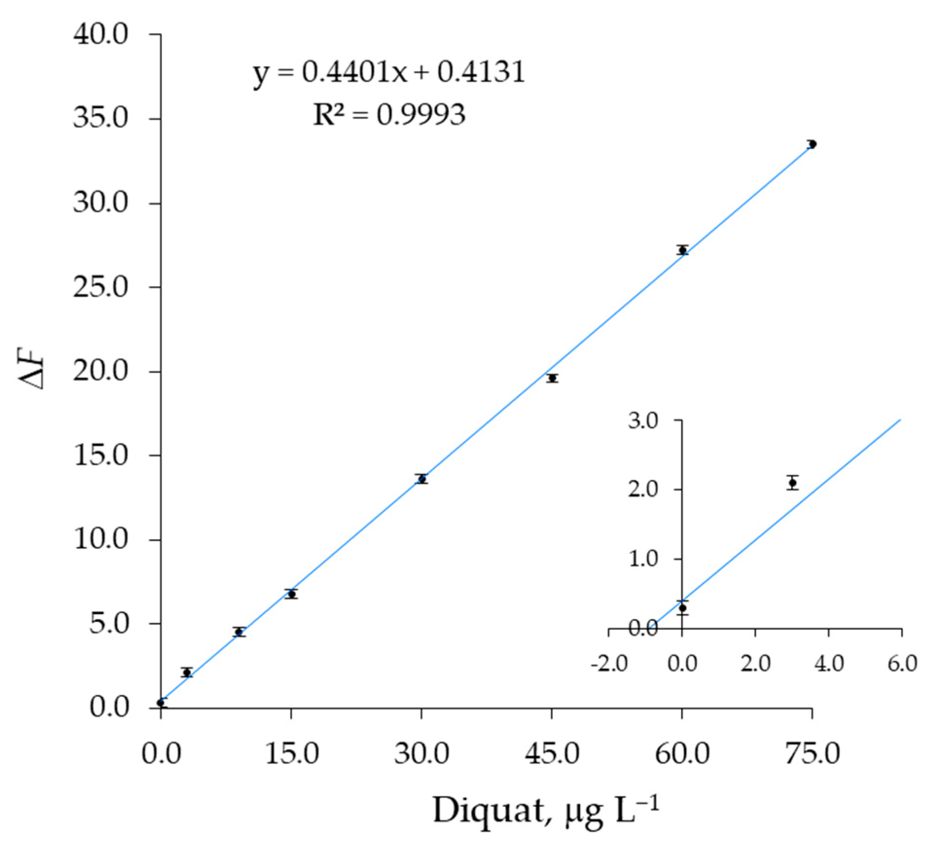
Figure 12.
Standard additions plot obtained by adding a methanol solution of diquat, DQ, and 1b to a tap water sample (3 replicates). The sample was divided into 8 equal aliquots. The spike concentration of 1.0 μg L−1 was normalized to the total volume of solvent, 60/40 methanol/water. Inset: The straight line intersects the x-axis to the value of (0.9 ± 0.1) μg L−1 of diquat.
Table 1.
Experimental data for the determination of spectra reported in
Figure 3. The
V1a and
VPQ volumes refer to an initial 1a solution with a concentration of 45.5 μg L
−1 and paraquat, PQ, solution with a concentration of 1000 μg L
−1, respectively. The final volume of each solution was made up to a total volume of 3000 μL by fixing with the solvent mixture.
| Entry | V1a, μL | VPQ, μL | VTOT, μL | [1a], μg L−1 | [PQ], μg L−1 | PQ/1a, mol/mol |
|---|
| 1 | 2000 | 0 | 3000 | 30.3 | 0.0 | 0.0 |
| 2 | 2000 | 2 | 3000 | 30.3 | 0.7 | 0.1 |
| 3 | 2000 | 4 | 3000 | 30.3 | 1.3 | 0.2 |
| 4 | 2000 | 7 | 3000 | 30.3 | 2.3 | 0.4 |
| 5 | 2000 | 11 | 3000 | 30.3 | 3.7 | 0.6 |
| 6 | 2000 | 16 | 3000 | 30.3 | 5.3 | 0.8 |
| 7 | 2000 | 20 | 3000 | 30.3 | 6.7 | 1.0 |
| 8 | 2000 | 27 | 3000 | 30.3 | 9.0 | 1.4 |
| 9 | 2000 | 35 | 3000 | 30.3 | 11.7 | 1.8 |
| 10 | 2000 | 45 | 3000 | 30.3 | 15.0 | 2.3 |
| 11 | 2000 | 53 | 3000 | 30.3 | 17.7 | 2.7 |
| 12 | 2000 | 65 | 3000 | 30.3 | 21.7 | 3.3 |
| 13 | 2000 | 75 | 3000 | 30.3 | 25.0 | 3.8 |
| 14 | 2000 | 92 | 3000 | 30.3 | 30.7 | 4.7 |
| 15 | 2000 | 105 | 3000 | 30.3 | 35.0 | 5.3 |
| 16 | 2000 | 115 | 3000 | 30.3 | 38.3 | 5.8 |
| 17 | 2000 | 132 | 3000 | 30.3 | 44.0 | 6.7 |
| 18 | 2000 | 152 | 3000 | 30.3 | 50.7 | 7.7 |
| 19 | 2000 | 192 | 3000 | 30.3 | 64.0 | 9.7 |
| 20 | 2000 | 252 | 3000 | 30.3 | 84.0 | 12.7 |
| 21 | 2000 | 332 | 3000 | 30.3 | 110.7 | 16.8 |
| 22 | 2000 | 432 | 3000 | 30.3 | 144.0 | 21.8 |
| 23 | 2000 | 572 | 3000 | 30.3 | 190.7 | 28.9 |
| 24 | 2000 | 772 | 3000 | 30.3 | 257.3 | 39.0 |
| 25 | 2000 | 932 | 3000 | 30.3 | 310.7 | 47.1 |
Table 2.
Experimental data for the determination of spectra reported in
Figure 4. The
V1b and
VPQ volumes refer to an initial 1b solution with a concentration of 50.7 μg L
−1 and paraquat, PQ, solution with a concentration of 1000 μg L
−1, respectively. The final volume of each solution was made up to a total volume of 4000 μL by fixing with the solvent mixture.
| Entry | V1b, μL | VPQ, μL | VTOT, μL | [1b], μg L−1 | [PQ], μg L−1 | PQ/1b, mol/mol |
|---|
| 1 | 2000 | 0 | 4000 | 25.4 | 0.0 | 0.0 |
| 2 | 2000 | 3 | 4000 | 25.4 | 0.8 | 0.1 |
| 3 | 2000 | 6 | 4000 | 25.4 | 1.5 | 0.3 |
| 4 | 2000 | 9 | 4000 | 25.4 | 2.3 | 0.4 |
| 5 | 2000 | 12 | 4000 | 25.4 | 3.0 | 0.6 |
| 6 | 2000 | 16 | 4000 | 25.4 | 4.0 | 0.8 |
| 7 | 2000 | 20 | 4000 | 25.4 | 5.0 | 0.9 |
| 8 | 2000 | 25 | 4000 | 25.4 | 6.3 | 1.2 |
| 9 | 2000 | 32 | 4000 | 25.4 | 8.0 | 1.5 |
| 10 | 2000 | 40 | 4000 | 25.4 | 10.0 | 1.9 |
| 11 | 2000 | 50 | 4000 | 25.4 | 12.5 | 2.4 |
| 12 | 2000 | 60 | 4000 | 25.4 | 15.0 | 2.8 |
| 13 | 2000 | 75 | 4000 | 25.4 | 18.8 | 3.5 |
| 14 | 2000 | 90 | 4000 | 25.4 | 22.5 | 4.3 |
| 15 | 2000 | 110 | 4000 | 25.4 | 27.5 | 5.2 |
| 16 | 2000 | 135 | 4000 | 25.4 | 33.8 | 6.4 |
| 17 | 2000 | 155 | 4000 | 25.4 | 38.8 | 7.3 |
| 18 | 2000 | 185 | 4000 | 25.4 | 46.3 | 8.7 |
| 19 | 2000 | 225 | 4000 | 25.4 | 56.3 | 10.6 |
| 20 | 2000 | 285 | 4000 | 25.4 | 71.3 | 13.5 |
| 21 | 2000 | 365 | 4000 | 25.4 | 91.3 | 17.3 |
| 22 | 2000 | 464 | 4000 | 25.4 | 116.0 | 21.9 |
| 23 | 2000 | 650 | 4000 | 25.4 | 162.5 | 30.7 |
| 24 | 2000 | 800 | 4000 | 25.4 | 200.0 | 37.8 |
| 25 | 2000 | 1000 | 4000 | 25.4 | 250.0 | 47.3 |
Table 3.
Experimental data for the determination of spectra reported in
Figure 5. The
V1a and
VDQ volumes refer to an initial 1a solution with a concentration of 45.5 μg L
−1 and diquat, DQ, solution with a concentration of 1650 μg L
−1, respectively. The final volume of each solution was made up to a total volume of 3000 μL by fixing with the solvent mixture.
| Entry | V1a, μL | VDQ, μL | VTOT, μL | [1a], μg L−1 | [DQ], μg L−1 | DQ/1a, mol/mol |
|---|
| 1 | 2000 | 0 | 3000 | 30.3 | 0.0 | 0.0 |
| 2 | 2000 | 10 | 3000 | 30.3 | 5.5 | 0.6 |
| 3 | 2000 | 30 | 3000 | 30.3 | 16.5 | 1.9 |
| 4 | 2000 | 50 | 3000 | 30.3 | 27.5 | 3.1 |
| 5 | 2000 | 80 | 3000 | 30.3 | 44.0 | 5.0 |
| 6 | 2000 | 100 | 3000 | 30.3 | 66.0 | 7.5 |
| 7 | 2000 | 120 | 3000 | 30.3 | 66.0 | 7.5 |
| 8 | 2000 | 170 | 3000 | 30.3 | 93.5 | 10.6 |
| 9 | 2000 | 230 | 3000 | 30.3 | 126.5 | 14.3 |
| 10 | 2000 | 300 | 3000 | 30.3 | 165.0 | 18.7 |
| 11 | 2000 | 380 | 3000 | 30.3 | 209.0 | 23.7 |
| 12 | 2000 | 470 | 3000 | 30.3 | 258.5 | 29.3 |
| 13 | 2000 | 570 | 3000 | 30.3 | 313.5 | 35.5 |
| 14 | 2000 | 660 | 3000 | 30.3 | 363.0 | 41.1 |
| 15 | 2000 | 780 | 3000 | 30.3 | 429.0 | 48.6 |
| 16 | 2000 | 870 | 3000 | 30.3 | 478.5 | 54.2 |
| 17 | 2000 | 950 | 3000 | 30.3 | 522.5 | 59.2 |
| 18 | 2000 | 1000 | 3000 | 30.3 | 550.0 | 62.3 |
Table 4.
Experimental data for the determination of spectra reported in
Figure 6. The
V1b and
VDQ volumes refer to an initial 1b solution with a concentration of 50.7 μg L
−1 and diquat, DQ, solution with a concentration of 1650 μg L
−1, respectively. The final volume of each solution was made up to a total volume of 4000 μL by fixing with the solvent mixture.
| Entry | V1b, μL | VDQ, μL | VTOT, μL | [1b], μg L−1 | [DQ], μg L−1 | DQ/1b, mol/mol |
|---|
| 1 | 2000 | 0 | 4000 | 25.4 | 0.0 | 0.0 |
| 2 | 2000 | 2 | 4000 | 25.4 | 0.8 | 0.1 |
| 3 | 2000 | 5 | 4000 | 25.4 | 2.1 | 0.3 |
| 4 | 2000 | 9 | 4000 | 25.4 | 3.7 | 0.5 |
| 5 | 2000 | 14 | 4000 | 25.4 | 5.8 | 0.8 |
| 6 | 2000 | 20 | 4000 | 25.4 | 8.3 | 1.2 |
| 7 | 2000 | 28 | 4000 | 25.4 | 11.6 | 1.6 |
| 8 | 2000 | 39 | 4000 | 25.4 | 16.1 | 2.3 |
| 9 | 2000 | 54 | 4000 | 25.4 | 22.3 | 3.1 |
| 10 | 2000 | 74 | 4000 | 25.4 | 30.5 | 4.3 |
| 11 | 2000 | 104 | 4000 | 25.4 | 42.9 | 6.1 |
| 12 | 2000 | 144 | 4000 | 25.4 | 59.4 | 8.4 |
| 13 | 2000 | 204 | 4000 | 25.4 | 84.2 | 11.9 |
| 14 | 2000 | 284 | 4000 | 25.4 | 117.2 | 16.6 |
| 15 | 2000 | 384 | 4000 | 25.4 | 158.4 | 22.4 |
| 16 | 2000 | 504 | 4000 | 25.4 | 207.9 | 29.4 |
| 17 | 2000 | 654 | 4000 | 25.4 | 269.8 | 38.1 |
| 18 | 2000 | 854 | 4000 | 25.4 | 352.3 | 49.8 |
| 19 | 2000 | 1254 | 4000 | 25.4 | 517.3 | 73.1 |
| 20 | 2000 | 1574 | 4000 | 25.4 | 649.3 | 91.8 |
Table 5.
Association constants of H-G complexes at 25 °C, reported as logK. Paraquat, PQ, and diquat, DQ, are the guests, G, and the compounds 1a and 1b are the fluorescent hosts, H. The values were determined by Equation (1). Uncertainties are given as standard deviation.
Table 5.
Association constants of H-G complexes at 25 °C, reported as logK. Paraquat, PQ, and diquat, DQ, are the guests, G, and the compounds 1a and 1b are the fluorescent hosts, H. The values were determined by Equation (1). Uncertainties are given as standard deviation.
| Guest | Host |
|---|
| 1a | 1b |
|---|
| DQ | 6.3 ± 0.3 | 6.7 ± 0.1 |
| PQ | 7.1 ± 0.1 | 7.3 ± 0.1 |
Table 6.
Association constants of H-G complexes at 25 °C, reported as logK. Paraquat, PQ, and diquat, DQ, are the guests, G, and the compounds 1a and 1b are the fluorescent hosts, H. The values were determined by Equation (3). Uncertainties are given as standard deviation.
Table 6.
Association constants of H-G complexes at 25 °C, reported as logK. Paraquat, PQ, and diquat, DQ, are the guests, G, and the compounds 1a and 1b are the fluorescent hosts, H. The values were determined by Equation (3). Uncertainties are given as standard deviation.
| Guest | Host |
|---|
| 1a | 1b |
|---|
| DQ | 6.4 ± 0.2 | 6.8 ± 0.1 |
| PQ | 7.2 ± 0.1 | 7.3 ± 0.1 |
Table 7.
Detection limits calculated for paraquat, PQ, and diquat, DQ, by fluorescence titration.
Table 7.
Detection limits calculated for paraquat, PQ, and diquat, DQ, by fluorescence titration.
| Guest | Host | m | Detection Limit, ng L−1 | λmax, nm |
|---|
| DQ | 1a | 1.3577 | 464 | 336 |
| DQ | 1b | 3.8479 | 164 | 416 |
| PQ | 1a | 6.5556 | 96 | 336 |
| PQ | 1b | 20.2826 | 31 | 416 |
Table 8.
Experimental data for the standard additions plot reported in
Figure 11.
V1b and
VPQ are the added volumes of the standard methanol solutions of [1b] = 2500 μg L
−1 and [PQ] = 1500 μg L
−1, respectively. A tap water sample was spiked and divided into 8 aliquots. The spike concentration of 1.0 μg L
−1 was normalized to the total volume of 2500 μL, 60/40 methanol/water.
| Entry | Vsample, μL | V1b, μL | VPQ, μL | VTOT, μL | [1b], μg L−1 | [PQ], μg L−1 | ΔF * |
|---|
| 1 | 1000 | 25 | 0 | 2500 | 25.0 | 0.0 | 2.4 |
| 2 | 1000 | 25 | 5 | 2500 | 25.0 | 3.0 | 11.3 |
| 3 | 1000 | 25 | 15 | 2500 | 25.0 | 9.0 | 28.1 |
| 4 | 1000 | 25 | 25 | 2500 | 25.0 | 15.0 | 44.8 |
| 5 | 1000 | 25 | 50 | 2500 | 25.0 | 30.0 | 85.0 |
| 6 | 1000 | 25 | 75 | 2500 | 25.0 | 45.0 | 136.0 |
| 7 | 1000 | 25 | 100 | 2500 | 25.0 | 60.0 | 174.1 |
| 8 | 1000 | 25 | 125 | 2500 | 25.0 | 75.0 | 212.9 |
Table 9.
Experimental data for the standard additions plot reported in
Figure 12.
V1b and
VDQ are the added volumes of the standard methanol solutions of [1b] = 2500 μg L
−1 and [DQ] = 1500 μg L
−1, respectively. A tap water sample was spiked and divided into 8 aliquots. The spike concentration of 1.0 μg L
−1 was normalized to the total volume of 2500 μL, 60/40 methanol/water.
| Entry | Vsample, μL | V1b, μL | VDQ, μL | VTOT, μL | [1b], μg L−1 | [DQ], μg L−1 | ΔF * |
|---|
| 1 | 1000 | 25 | 0 | 2500 | 25.0 | 0.0 | 0.3 |
| 2 | 1000 | 25 | 5 | 2500 | 25.0 | 3.0 | 2.1 |
| 3 | 1000 | 25 | 15 | 2500 | 25.0 | 9.0 | 4.5 |
| 4 | 1000 | 25 | 25 | 2500 | 25.0 | 15.0 | 6.8 |
| 5 | 1000 | 25 | 50 | 2500 | 25.0 | 30.0 | 13.6 |
| 6 | 1000 | 25 | 75 | 2500 | 25.0 | 45.0 | 19.6 |
| 7 | 1000 | 25 | 100 | 2500 | 25.0 | 60.0 | 27.2 |
| 8 | 1000 | 25 | 125 | 2500 | 25.0 | 75.0 | 33.5 |
Table 10.
Inorganic species detected in the tested sample of tap water and their effect on the determination of herbicide in a solution of these ions with a 10-fold higher concentration.
Table 10.
Inorganic species detected in the tested sample of tap water and their effect on the determination of herbicide in a solution of these ions with a 10-fold higher concentration.
| Species | Amount, mg L−1 of Tested Sample | Addition 1 for 10.0 mL | Signal Variation, % |
|---|
| Ca2+ | 42.1 | 10.52 mg, as CaCO3 | 2 |
| Mg2+ | 12.3 | 4.89 mg, as MgCl2 | 2 |
| Zn2+ | 0.8 | 0.35 mg, as ZnSO4·7H2O | 4 |
| Na+ | 39.4 | 0.70 mg, as NaCl | <1 |
| 3.23 mg, as Na2SO4 |
| 0.03 mg, as Na3PO4 |
| 6.03 mg, as Na2CO3 |
| K+ | 3.1 | 0.81 mg, as KNO3 | <1 |
| SO42− | 23.0 | 3.23 mg, as Na2SO4 | 3 |
| 0.35 mg, as ZnSO4·7H2O |
| PO43− | 0.2 | 0.03 mg, as Na3PO4 | 2 |
| NO3− | 5.0 | 0.81 mg, as KNO3 | 4 |
| CO32− | 98.0 | 10.52 mg, as CaCO3 | 4 |
| 6.03 mg, as Na2CO3 |
| Cl− | 40.3 | 4.89 mg, as MgCl2 | 3 |
| 0.70 mg, as NaCl |
Table 11.
Experimental data for the selectivity evaluation of the PQ-1b probe in the presence of diquat as interferent. The signal variation was calculated in the linear range from 1.0 to 10.0 μg L−1 according to Equation (6), comparing F0, the maximum fluorescence intensity of a paraquat solution, with F, the maximum fluorescence intensity of an equimolar solution of paraquat and diquat. The fluorescence values were measured at 416 nm for anthracene fluorophore 1b.
| Entry | [1b], μg L−1 | [PQ], μg L−1 | F0 | [DQ], μg L−1 | F | Signal Variation, % |
|---|
| 1 | 25.0 | 0.0 | 418.0 | 0.0 | 418.0 | 0.0 |
| 2 | 25.0 | 1.0 | 396.5 | 1.0 | 392.4 | 1.0 |
| 3 | 25.0 | 2.0 | 376.4 | 2.0 | 373.2 | 0.9 |
| 4 | 25.0 | 3.0 | 356.2 | 3.0 | 353.5 | 0.8 |
| 5 | 25.0 | 5.0 | 315.5 | 5.0 | 312.7 | 0.9 |
| 6 | 25.0 | 7.0 | 275.1 | 7.0 | 273.0 | 0.8 |
| 7 | 25.0 | 10.0 | 214.3 | 10.0 | 212.8 | 0.7 |
Table 12.
Experimental data for the evaluation of cross-interferences by using the standard addition method. V1b, VDQ and VPQ are the added volumes of the standard methanol solutions of [1b] = 2500 μg L−1, [DQ] = 3000 μg L−1 and [PQ] = 1500 μg L−1, respectively. VPQ-spike and VDQ-spike are the volumes added to a tap water sample to spike it at the concentration of 6.0 μg L−1. This value was normalized to the total volume of 2500 μL, 60/40 methanol/water. The sample was divided into 10 aliquots.
| Entry | Vsample, μL | V1b, μL | VPQ-spike,
μL | VDQ-spike, μL | VDQ, μL | VTOT, μL | [1b], μg L−1 | [PQ]spike, μg L−1 | [DQ]spike, μg L−1 | [DQ], μg L−1 | ΔF * |
|---|
| 0 | 1000 | 30 | 0 | 0 | 0 | 2500 | 30.0 | 0.0 | 0.0 | 0.0 | 0.0 |
| 1 | 1000 | 30 | 10 | 5 | 0 | 2500 | 30.0 | 6.0 | 6.0 | 0.0 | 17.9 |
| 2 | 1000 | 30 | 10 | 5 | 5 | 2500 | 30.0 | 6.0 | 6.0 | 6.0 | 18.2 |
| 3 | 1000 | 30 | 10 | 5 | 15 | 2500 | 30.0 | 6.0 | 6.0 | 18.0 | 19.2 |
| 4 | 1000 | 30 | 10 | 5 | 30 | 2500 | 30.0 | 6.0 | 6.0 | 36.0 | 21.9 |
| 5 | 1000 | 30 | 10 | 5 | 50 | 2500 | 30.0 | 6.0 | 6.0 | 60.0 | 29.1 |
| 6 | 1000 | 30 | 10 | 5 | 75 | 2500 | 30.0 | 6.0 | 6.0 | 90.0 | 41.9 |
| 7 | 1000 | 30 | 10 | 5 | 100 | 2500 | 30.0 | 6.0 | 6.0 | 120.0 | 55.6 |
| 8 | 1000 | 30 | 10 | 5 | 125 | 2500 | 30.0 | 6.0 | 6.0 | 150.0 | 68.4 |
| 9 | 1000 | 30 | 10 | 5 | 150 | 2500 | 30.0 | 6.0 | 6.0 | 180.0 | 81.7 |


