
Microstrip Antenna Development for Radar Sensor
Department of Broadband Infocommunications and Electromagnetic Theory, Budapest University of Technology and Economics, Műegyetem rkp 3, H-1111 Budapest, Hungary
Sensors 2023, 23(2), 909; https://doi.org/10.3390/s23020909
Submission received: 12 December 2022
/
Revised: 9 January 2023
/
Accepted: 10 January 2023
/
Published: 12 January 2023
(This article belongs to the Collection RF and Microwave Communications)
Abstract
:Tank level measurement is an important research area in radar technology. Level measurement using radar technology is a safe solution even under extreme process conditions, such as high pressure, temperature, and vapors. Special antennas are required to meet electromagnetic requirements such as high gain, low sidelobe level, and high bandwidth. Another requirement is a small size and good manufacturability of the antenna. One promising solution is the use of microstrip antennas for tank-level measurements. This paper presents a special microstrip antenna, that meets the main requirements in addition to a circular antenna layout, which fills optimally the tank hatch. To do this, we created a special antenna layout with a suitable feeding network and added an optimized ring around the antenna system, which significantly reduces the sidelobe level. The center frequency of the antenna is 25 GHz with a 1 GHz bandwidth.
1. Introduction
Constant product quality, operational safety, and economic efficiency can only be ensured by continuous measurements and intervention and control systems based on these measurements. Liquids, pastes, bulk solids, and liquefied gases are most often stored in tanks, silos, or mobile containers. These tanks are used in the chemical and petrochemical industries, the pharmaceutical and life sciences industries, the water industry, the chemical and petrochemical industries, the water and wastewater, and the food and energy industries.
There are several classical and modern methods for measuring the product level in process and storage tanks. Applications are in the chemical, petrochemical, pharmaceutical, water, and food industries, mobile tanks on vehicles and ships, and natural reservoirs such as seas, dams, lakes, and oceans. Typical tank heights range from 0.5 m to 37 m. [1,2]
Two main measurement tasks can be distinguished [3]:
- continuous level measurement, i.e., level indication,
- level detection, i.e., detection of an alarm limit to prevent overfilling.
Many level devices are mounted on top of the tank and measure primarily the distance between their mounting position and the product’s surface [3] (Figure 1).
For level measurement, a significant number of different principles measurement techniques are available [4], and it is advisable to select the optimum technique and sensor. The commonly used tank-level measurement methods are based on the next basic principles: buoyant object floats, RF capacitance, radar, ultrasonic, and hydrostatic head/tank gauging. No single principle applies to all measurement areas. Therefore, measurement systems should be selected based on what works reliably under the given conditions, and at the same time meet the accuracy of the measurement.
We developed a sensor antenna for radar-level pulse [5] measurement, which is based on the principle that the time required for the propagation of microwaves. It is the time takes for the wave packet to travel during the entire round trip between the non-contact transducer detected material level and the measuring device. Pulse radar has been widely used for distance measurement since the early days of radar. Radar level measurement is a safe non-contact solution even under extreme process conditions, at high pressure, and temperature, vapors. For radar measurements, special antennas are required to meet electromagnetic requirements such as high gain, low sidelobe level, and high bandwidth. Another requirement is a small size and good manufacturability of the antenna.
A promising solution is the use of microstrip antennas [6,7,8,9] for contactless tank level measurement. Its main advantages are the small height and weight, and easy manufacturability.
Many other antenna types are promising for tank-level radar measurements, such as conical horn antennas [10], parabolic reflector antennas [11], and dielectric antennas [12,13,14].
Recently, theoretical work is conducted applying metamaterial-based antennas [15] also for tank-level measuring sensor antennas. These analytical or numerical solutions allow for the designing and building of useful antennas and devices; however, more effective fabrication techniques need to be developed for these devices. Another difficulty of the metamaterial type antennas is the bandwidth because these devices show generally narrowband behavior and bandwidth is not analyzed [15].
In this paper, a special microstrip antenna was designed, that meets the main requirements, i.e., high gain, low sidelobe level, high bandwidth, small size, and good manufacturability of the antenna. The antenna was realized on a low-loss RT5880 substrate. As opposed to the traditional N × N microstrip antenna layout, we used a special 24-element layout. With this arrangement, the side beam suppression has been significantly reduced. The feeding network of the 24-element antenna system is made up of three main power-divider elements, with three different power-division ratios. CST Microwave Studio was used to simulate and fine-tune the antenna array. The measurements were performed in an anechoic chamber, where we measured input reflection and antenna radiation patterns in the 23–27 GHz frequency range.
2. Antenna Design
The special microstrip antenna satisfies two main requirements, namely a circular antenna layout and an optimized ring around the antenna system, which significantly reduces the sidelobe level. The center frequency of the antenna is 25 GHz with a bandwidth of 1 GHz.
In this chapter, the design of the feeding network for a microstrip antenna system with a 24-element circular confinement geometry is presented in detail as the optimization of the sideband suppression ring. The electromagnetic design of the antenna was carried out using the Ansys Designer 2D planar [16] and CST Microwave Studio 3D [17] software.
To fulfill the requirements an antenna system will be introduced, which optimally fills the standard circular opening of the tanks. The sizes of the antenna designed were chosen to fit into and optimally fill the standard circular opening of the tanks (Figure 2).
The feeding network is designed for the antenna system for optimal illumination. We introduce the detailed design process of the microstrip antenna element, placing, and feeding network. (Figure 3)
2.1. Single Radiator—Microstrip Patch
With the development of modern wireless communications and radar technology, there is an increasing demand for compact antennas. Microstrip Patch Antennas (MPA) are lightweight, low cost, and easy to integrate into microwave circuits, and are therefore widely used in mobile and wireless applications. The use of MPAs in mobile wireless communication systems allows the implementation of small, low antenna sizes [18,19].
The basic geometry of the antenna is a dielectric substrate located between the ground plane and the radiating patch. The size and shape of the MPA radiator, as well as the height and the type of substrate material, are the most important design parameters for evaluating the performance of an MPA. The substrate, in addition to providing mechanical strength to the entire antenna, also allows the propagation of surface waves. The dielectric substrate layer separates the radiator from the ground, its material and thickness are of primary importance for the antenna bandwidth. Since the antenna dimensions are finite, the fields along the antenna are finite, and the fields along the edges are frictional [19].
Several authors have investigated the effect of substrate thickness and material on the bandwidth of MSA. We simulated a single MPA (Figure 4) to test its relative bandwidth and radiation efficiency for three substrates and five heights of substrates [20,21,22,23,24,25,26,27,28].
The substrates investigated were Rogers RT5880, RO4003, and RO3010 with substrate heights of 5, 10, 20, 31, and 62 mils. The simulation results are summarized in Table 1.
Table 1 clearly shows that antenna bandwidth can be increased by increasing the substrate height but the efficiency of the antenna changes in the opposite direction. The goal of 1 GHz bandwidth (4%) can be achieved as Table 1 shows. The candidate is an RT5880 substrate with either 20 or 31 mils of height for the best radiation efficiency. Finally, the following standard 31mil substrate thickness was chosen to compensate for bandwidth loss due to manufacturing errors of antennas and feeding networks.
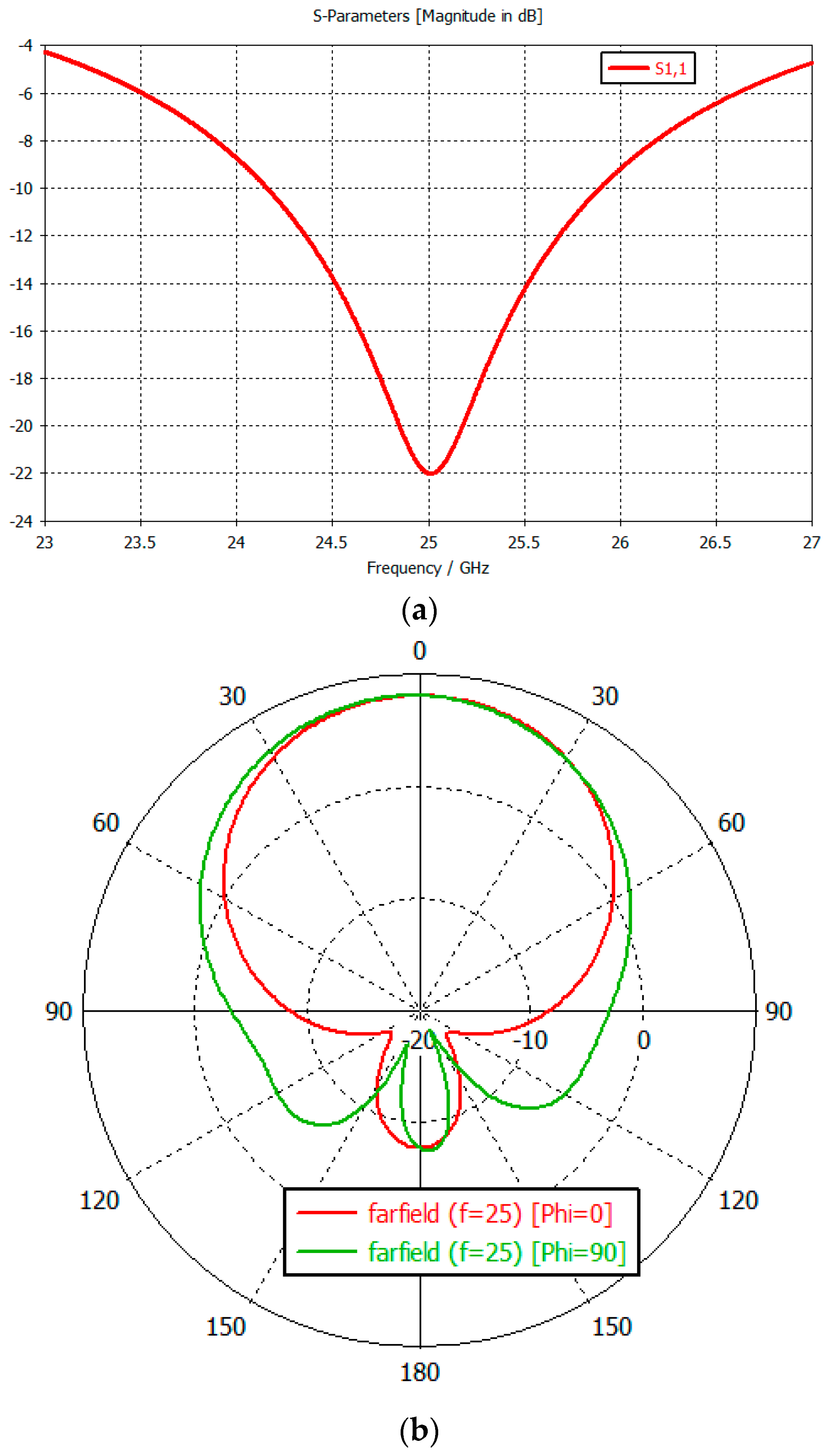
The single MPA antenna, simulated on 31mils RT5880 substrate, input reflection, and radiation pattern are shown in Figure 5.
The single radiator has 8 dB gain at 25 GHz and 80.7° and 72.7° beamwidth in E and H planes (Figure 5b).
The next design step is the radiator array structure design.
2.2. The Radiator Array Structure
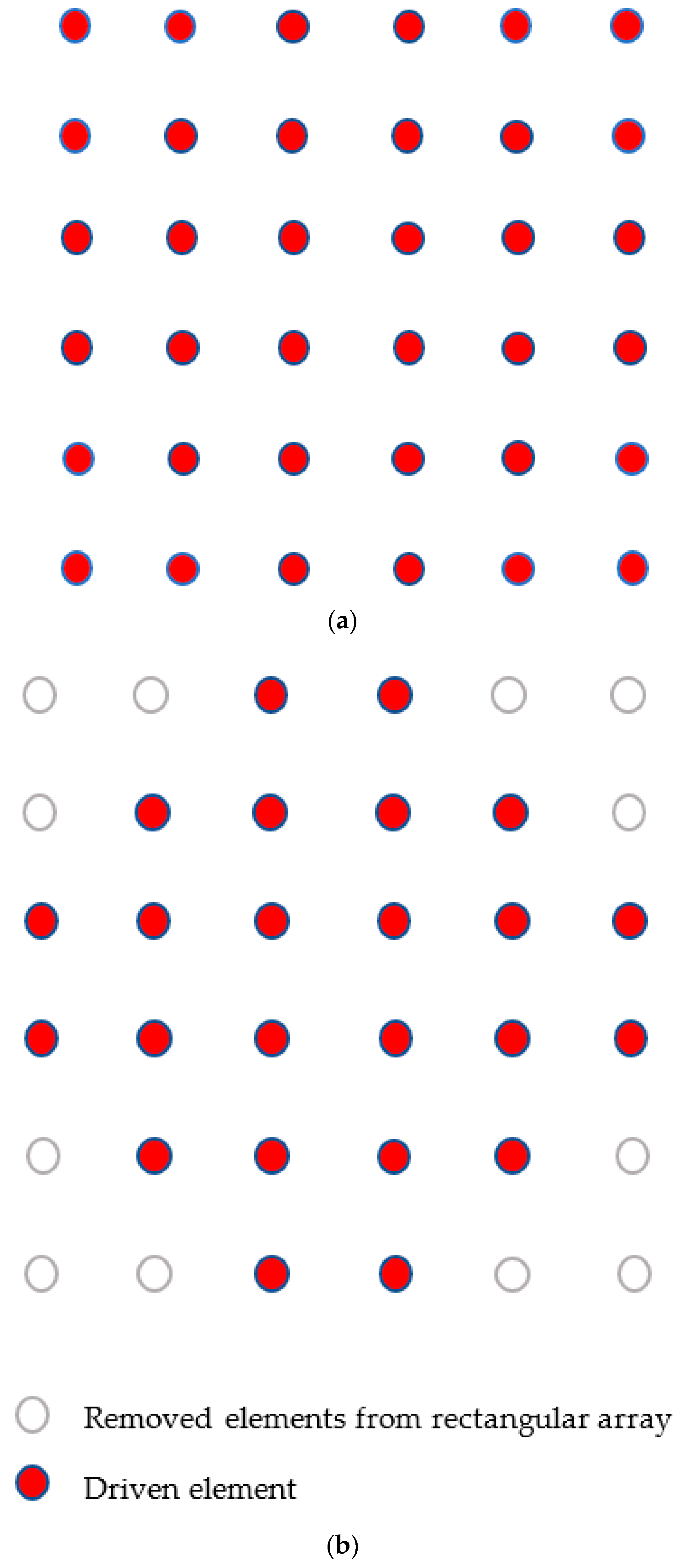
The excitation of each radiator, which can be of uniform or non-uniform amplitude, is adjusted by the feeding network. We first examined a 6 × 6 planar array of uniform rectangular shape and a special 24-element array. (Figure 6)
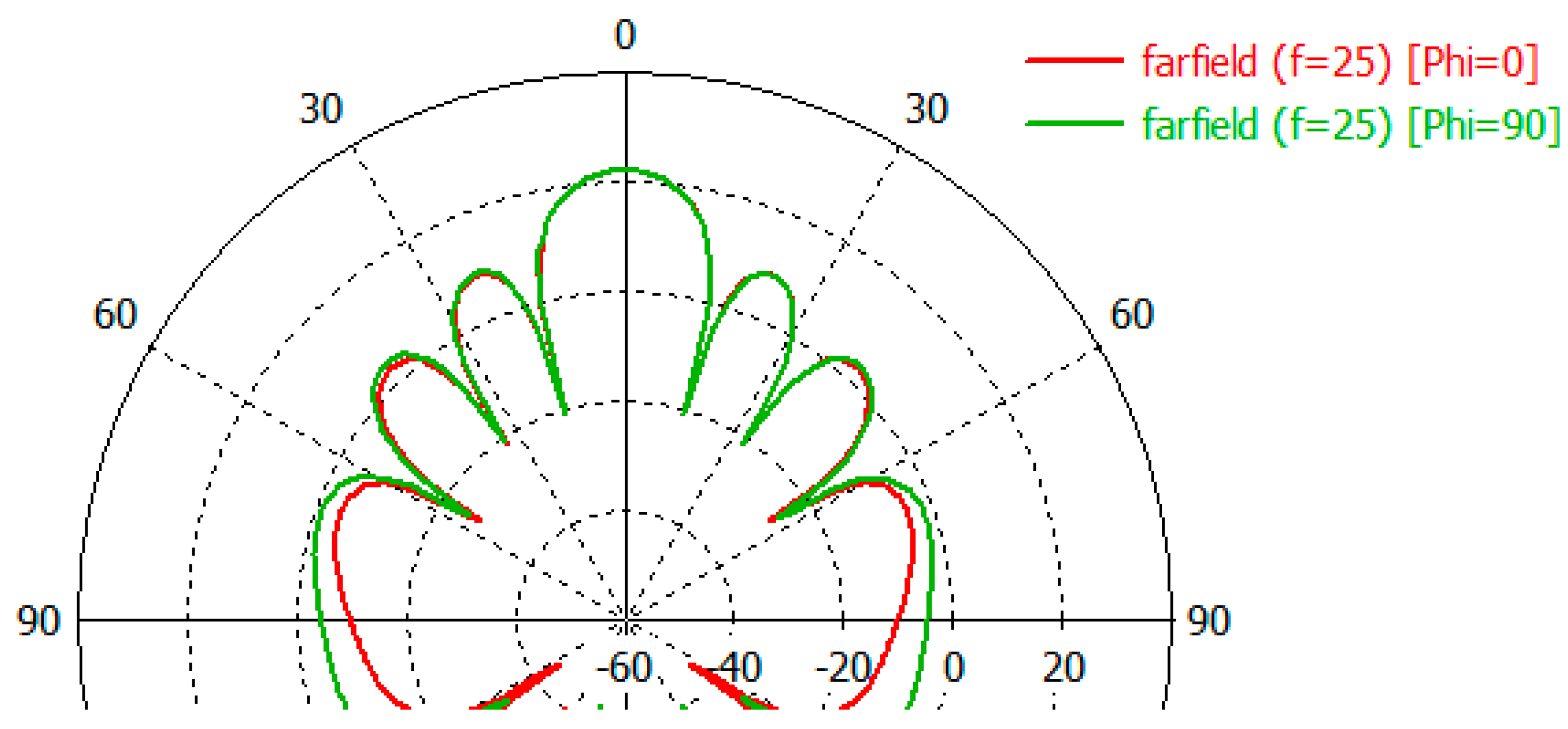
The directional characteristics of the two arrays were compared using the CST array simulator. The radiation pattern for the 6x6 uniform and 24 elements arrays can be seen in Figure 7 and Figure 8.
The main point of comparison was the Sidelobe Level. (Table 2) The 24 elements array has a 2.1dB better SLL.
The final arrangement of microstrip radiators in the Ansys Designer simulator can be seen in Figure 9.
The antenna-connected transmission lines in Figure 9 have already been arranged for the optimal feeding network.
2.3. Feeding Network
The feeding network is made up of three main elements. We implemented three different power division ratios [29].
The design of the power dividers was based on the simple T-junction.
The power dividers are the following:
Power divider for 1 to 4 power ratio (Figure 10),
3-way power divider from 1 to 4:2:4 power ratio (Figure 11),
4-way power divider from 1 to 2:10:10:2 power ratio (Figure 12).
After calculating the elements of the power dividers, we used Ansys Designer/Nexxim [17] for the final design and analysis of the three main elements of the feeding network. The design was carried out in two steps, first, the circuit model simulator was used to set the matching and power ratio using the ideal transmission line transformers, and then the 2.5D simulator was used to optimize the layout with microstrip transmission lines. Each of the corners was mitered to reduce the reflection.
2.3.1. Power Division Network for the 1 to 4 Power Ratio
The purpose of this network is to feed four identical radiators with the same power and phase. The single microstrip radiator has a 120 ohms input impedance at a center frequency of 25 GHz.
Finally, at the planar feeding network design, a transmission line step was introduced between the microstrip radiator and the T-matching element (Figure 10b).
The resonance frequency of the power division network for the 1 to 4 power ratio was set to 25 GHz (Figure 11).
Figure 12 shows the power ratio for the four radiators of the power division network for the 1 to 4 power ratio. The −6.025 dB power transfer means that the network results in a 1:4 power division with a −0.025 dB loss. Transmission lines in the circuit models are ideal but lossy.
2.3.2. Power Division Network from 1 to 4:2:4 Power Ratio
The upper part of the network feeds 2 × 4 + 2 antennas with the same power. The 2 × 4 feeding part consists of two power division networks for a 1 to 4 power ratio.
The design of the three ways power dividers was based on two equations, the impedance matching equation, and the power ratio equation.
The equation for impedance match:
where
the divider input impedance (40 ohms),
the impedance of ways 1 and the impedance of way 2.
The power sum equation:
The power ratio R:
Solving Equations (2) and (3) gives
For matching, we applied a 141.2 ohms quarter wavelength transformer between 100 ohms, 200 ohms, and 109.55 ohms quarter wavelengths transformer between 120 ohms and 100 ohms (Figure 13a).
The circuit model of the power division network from 1 to 4:2:4 power ratio can be seen in Figure 13a and the layout with the microstrip radiators is shown in Figure 13b.
The resonance frequency of the power division network for 1 to 4:2:4 power ratio was set to 25 GHz and the input reflection is shown in Figure 14.
The Figure 15. Shows the power ratio for the radiators of the power division network from 1 to 4:2:4 power ratio. The −10 dB power transfer means that the network results in a 1:10 power division with less than 0.1 dB power transfer difference in the bandwidth of 24.5–25.5 GHz.
2.3.3. Power Division Network from 1 to 2:10:10:2 Power Ratio
The final part of the feeding network design was the 24 elements’ feeding structure. This power divider is a four ways circuit with a 1 to 2:10:10:2 power ratio.
The design of the power divider was based on two equations, the impedance matching equation, and the power ratio equation.
The equation for impedance matching:
where
the antenna input impedance, 50 ohms,
the impedance of ways 1 and the impedance of way 2.
The power sum equation:
The power ratio:
Solving equations gives
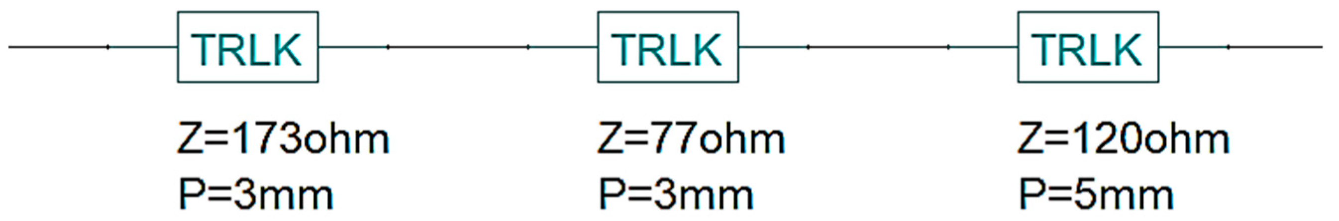
The 600 ohms microstrip transmission line is difficult to implement because of its small width, therefore we implemented two-stage quarter wavelength transformers between 120 ohms and 600 ohms. Our technology makes it possible to realize less than 200 ohms of microstrip transmission lines. The two-quarter wavelength transformers’ characteristic impedances are 77 and 173 ohms (Figure 16).
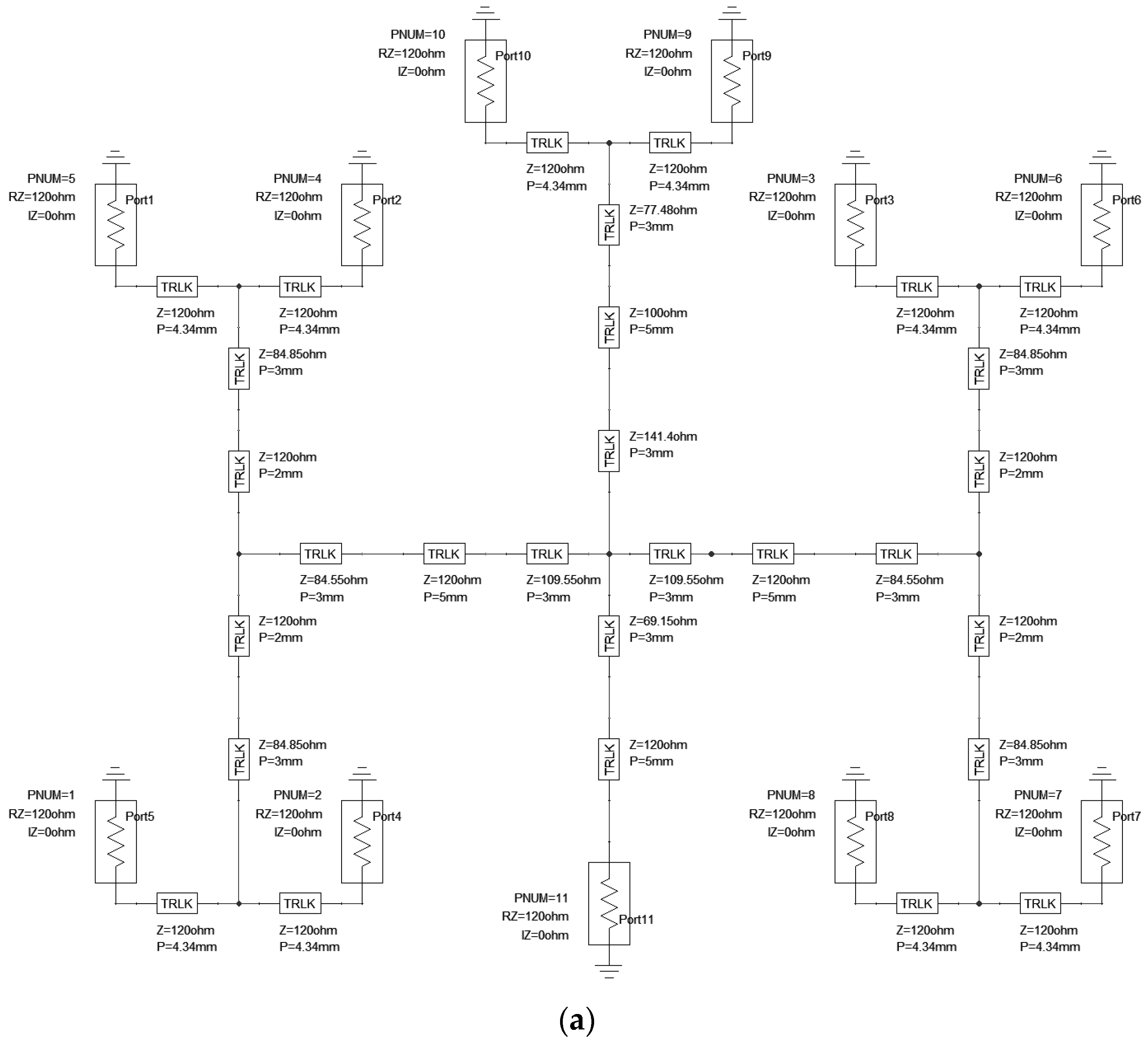
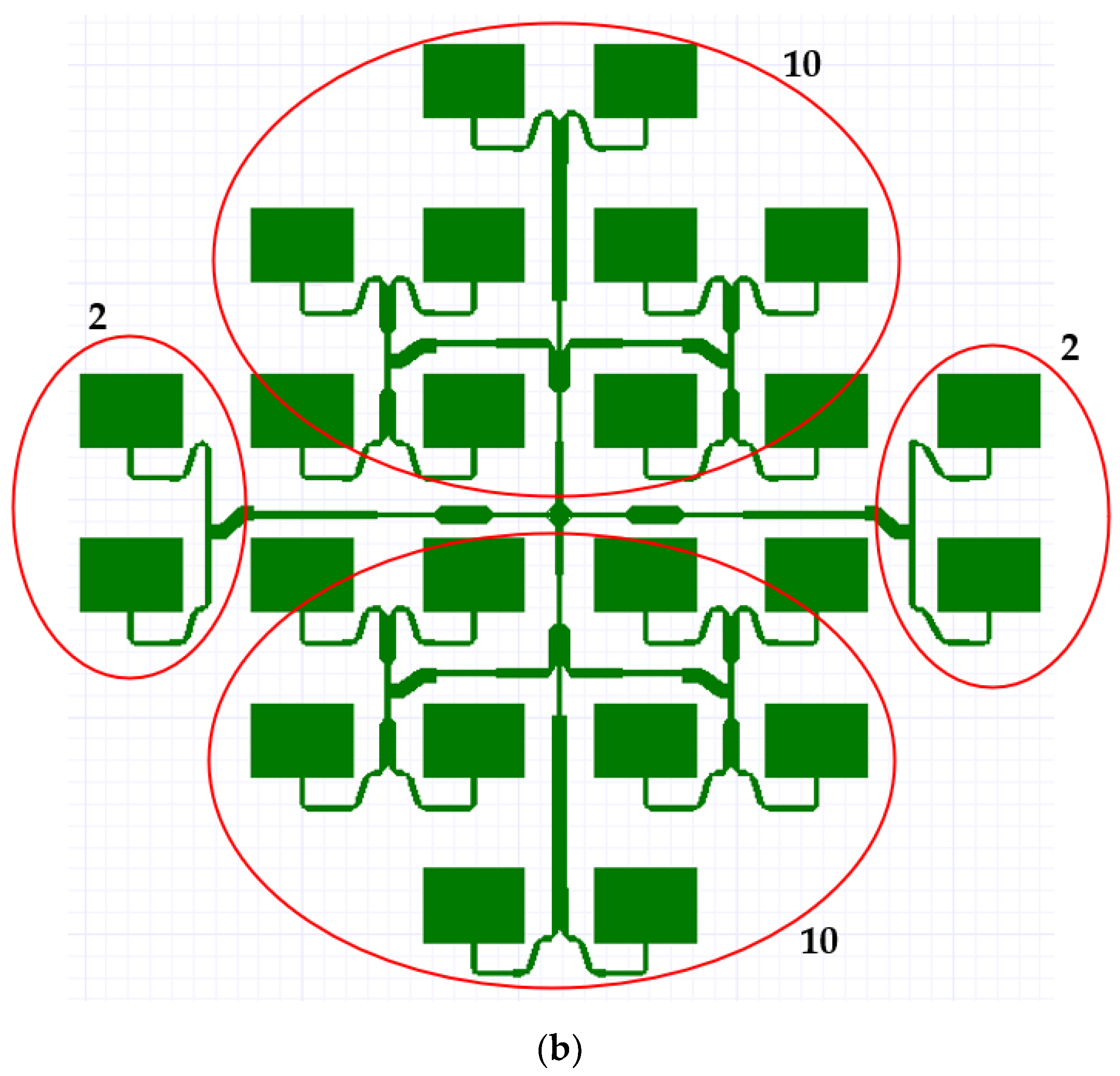
The whole system is symmetrical in the horizontal plane and is completed by an additional 2 × 2 elements left and right (Figure 17).
The resonance frequency of the power division network for 1 to 2:10:10:2 power ratio was set to 25 GHz and the input reflection is shown in Figure 18.
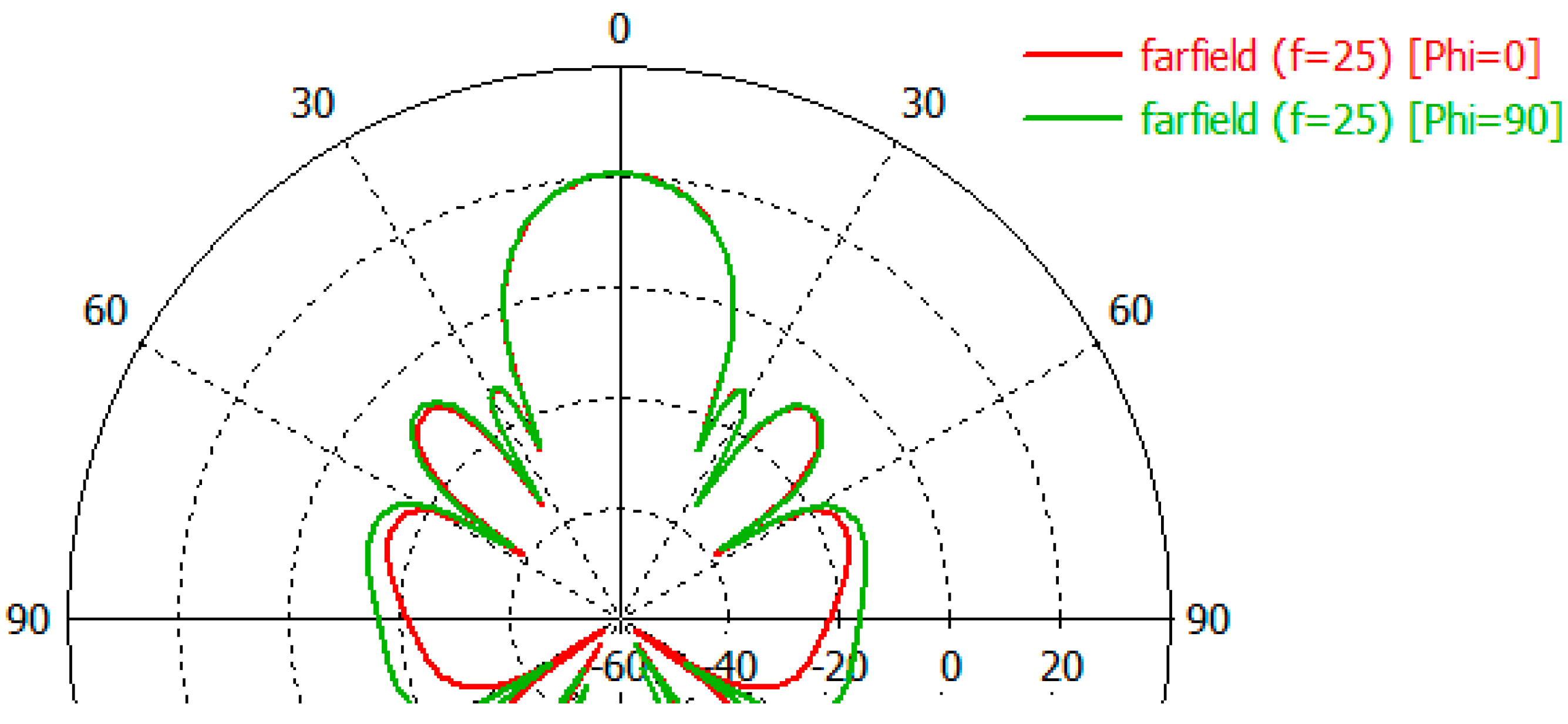
Figure 19 shows the power ratio for the radiators of the power division network from 1 to 2:10:10:2 power ratio. The 1:24 power division with less than 0.15 dB power transfer difference at 25 GHz center frequency and less than 0.35 dB power transfer difference in the bandwidth of 24.5–25.5 GHz.
3. Results
After the design and optimization of the feeding network, the CST Microwave Studio was used for the simulation and fine-tuning of the antenna array (Figure 19). Our most important technical parameters were the input reflection bandwidth and the SLL [30,31,32,33].
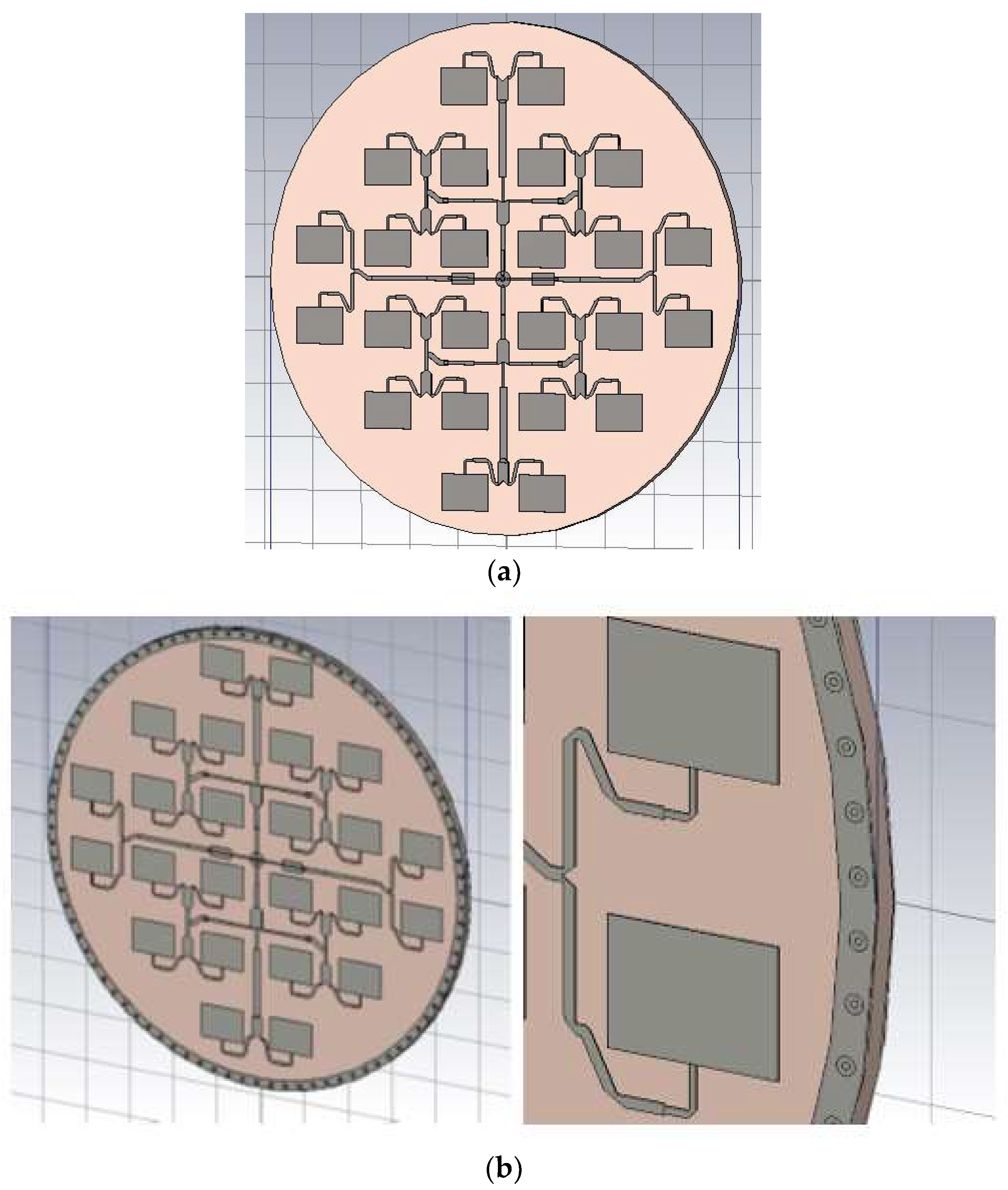
Two versions of antennas were investigated. After the first simulation was found, that the SLL is not acceptable in some directions, therefore an optimized ring with ground vias was implemented, to increase the antenna sidelobe level (SLL) (Figure 20b).
Examination of the radiation patterns showed that the SLL could be reduced by up to 5 dB in some directions by using the ring. The antenna gain is not changed significantly. The SLL reduction was significant in the Phi = 0 plane in the elevation angle range of 50–180 degrees (Figure 21). Here the SLL reduction was around 5 dB. On the other plane in the Phi = 90 the SLL reduction can be experienced only at back range (Figure 22).
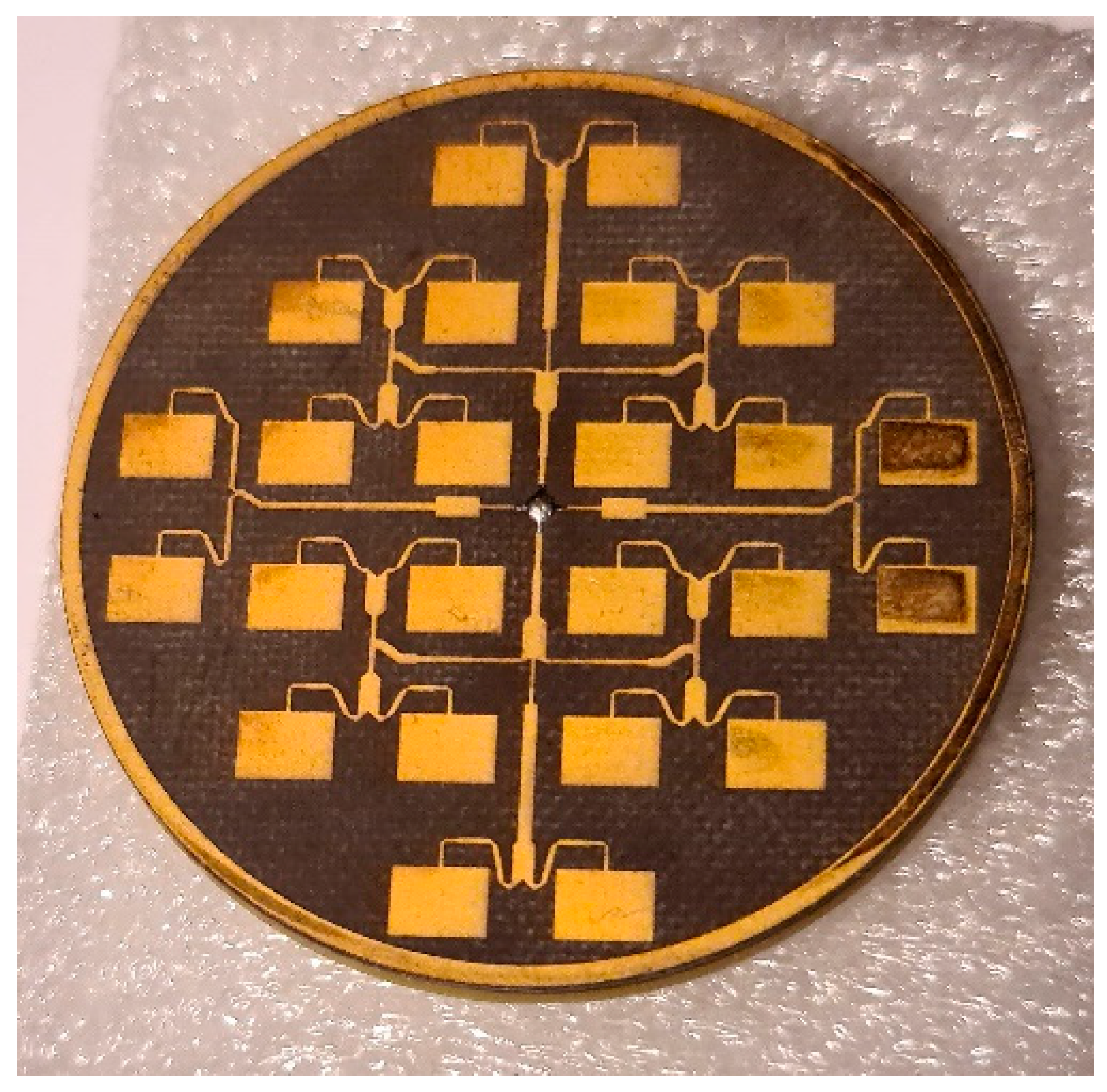
After simulation verification of the antenna’s functionality, the antenna was built (Figure 23).
For the measurements, an SMA connector was connected to the antenna input with a semirigid coaxial transmission line, and a radome was applied (Figure 24).
The measurements were performed in the antenna measurement room of the Department of Broadband Infocommunications and Electromagnetic Theory of the Budapest University of Technology.
The antenna input reflection in the 23–27 GHz frequency band shows a good agreement between simulated and measured values (Figure 25).
The antenna radiation pattern was measured in the two main planes and the results show SLL better than −17.3 dB (Figure 26).
Finally, we compared and summarized the most important antenna radiation pattern characteristics in Table 3.
It can be concluded that the parameters of the antenna have been measured and verified to meet the specification. The parameters were achieved by using a special feeding network and a sidelobe suppression ring.
4. Conclusions and Future Work
We presented a systematic design of a microstrip antenna array and its feeding network. A new antenna layout was proposed for the tank level meter radar sensor. The microstrip antenna elements optimally fill the opening of the tank, therefore maximal gain can be reached. The optimized outer ring ensures the improved sidelobe level to reduce the side reflections from tank sidewalls. The correctness of the design was verified by measurements.
We plan to investigate the antenna further, mainly to improve the feeding network with non-uniform illumination. Another possibility for further development is the use of artificial material as the sidelobe suppression ring.
Funding
This research was funded by the Hungarian Fund 2020-1.1.2-PIACI-KFI-2021-00278.
Acknowledgments
The author very much appreciates the support from the NIVELCO Process Control Co. and the infrastructure of the Department of Broadband Infocommunication and Electromagnetic Theory at the Budapest University of Technology and Economics.
Conflicts of Interest
The authors declare no conflict of interest.
References
- Water Storage Tank Models—Roof Types. Available online: https://waterstoragetanksinc.com/water-tank-models/ (accessed on 15 December 2022).
- Reservoirs and Standpipes Water Storage, McDermott. Available online: https://www.mcdermott.com/getmedia/b9244931-3d69-4510-9c41-185b577ab36a/Reservoirs-and-Standpipes-Water-Storage-Brochure.pdf.aspx (accessed on 15 December 2022).
- Webster, J.G. The Measurement, Instrumentation and Sensors Handbook, 1st ed.; CRC Press LLC: Boca Raton, FL, USA, 1999. [Google Scholar]
- Vass, G. The Principles of Level Measurement. Available online: https://www.fierceelectronics.com/sensors/bmws-i-vision-dee-concept-car-can-talk-and-offers-32-swappable-exterior-colors (accessed on 15 December 2022).
- Application Brief—Radar Pulse Measurements Challenges. Available online: https://dl.cdn-anritsu.com/en-us/test-measurement/files/Application-Notes/Application-Note/11410-00708A.pdf (accessed on 15 December 2022).
- 2-Wire Non-Contact Radar (FMCW) Level Meter. Available online: https://www.inducont.lv/res/dwn/krohne/BM702A.pdf (accessed on 15 December 2022).
- Pozar, D.M. Microstrip antennas. Proc. IEEE 1992, 80, 79–91. [Google Scholar] [CrossRef]
- Pozar, D.M.; Schaubert, D.H. Microstrip Antennas: The Analysis and Design of Microstrip Antennas and Arrays, 1st ed.; Wiley-IEEE Press: Hoboken, NJ, USA, 1995. [Google Scholar] [CrossRef]
- Carver, K.R.; Mink, J.W. Microstrip antenna technology. IEEE Trans. Antennas Propag. 1981, AP-29, 2–24. [Google Scholar] [CrossRef]
- Bahl, I.J.; Bhartia, P. MicrostripAntennas, 1st ed.; Artech House: Dedham, MA, USA, 1980. [Google Scholar]
- Rosemound TankRadar PRO, Technical Description. Available online: https://www.pico.co.th/img/prod-Wireless-20TankRadar-20PRO.pdf (accessed on 15 December 2022).
- PiloTREK, K-Band Radar Liquids. Available online: https://www.nivelco.com/public/files/documents/735b8dff-68eb-4fe8-8e53-47ae6bc03e38/we10s17a0605b.pdf (accessed on 15 December 2022).
- Gerding, M.; Much, T.; Nils, P. Dielectric Antenna. U.S. Patent 8,242,965, 14 August 2012. Available online: https://patents.justia.com/patent/8242965 (accessed on 15 December 2022).
- Pohl, N.; Gerding, M. A dielectric lens-based antenna concept for high-precision industrial radar measurements at 24 GHz. In Proceedings of the 9th European Radar Conference, Amsterdam, The Netherlands, 31 October–2 November 2012; pp. 405–408. [Google Scholar] [CrossRef]
- Pohl, N.; Gerding, M. A dielectric lens-based antenna concept for high-precision industrial radar measurements at 24 GHz. In Proceedings of the 42nd European Microwave Conference, Amsterdam, The Netherlands, 29 October–1 November 2012; pp. 731–734. [Google Scholar] [CrossRef]
- Palmeri, R.; Bevacqua, M.T.; Morabito, A.F.; Isernia, T. Design of Artificial-Material-Based Antennas Using Inverse Scattering Techniques. IEEE Trans. Antennas Propag. 2018, 66, 7076–7090. [Google Scholar] [CrossRef]
- ANSYS Designer/Nexxim 2014. Available online: https://www.inas.ro/files/docs/ansys/ansys-designerrf.pdf (accessed on 15 December 2022).
- CST Studio Suite Electromagnetic Field Simulation Software. Available online: https://www.3ds.com/products-services/simulia/products/cst-studio-suite/ (accessed on 15 December 2022).
- Ma, M.T. Theory and Application of Antenna Arrays, 1st ed.; Wiley-Interscience Publication: New York, NY, USA, 1974. [Google Scholar]
- James, J.R.; Hall, P.S.; Wood, C. Microstrip Antenna Theory and Design, 1st ed.; Peter Peregrinus: London, UK, 1981. [Google Scholar]
- Pozar, D.M.; Kaufman, B. Increasing the bandwidth of a microstrip antenna by proximity coupling. Electron. Lett. 1987, 23, 368–369. [Google Scholar] [CrossRef]
- Henderson, A.; James, J.R.; Hall, C.M. Bandwidth extension techniques in printed conformal antennas. In Proceedings of the Military Microwaves, MM 86, Brighton, England, 24–26 June 1986; pp. 329–334. [Google Scholar]
- Pozar, D.M.; Kaufman, B. Design considerations for low sidelobe microstrip arrays. IEEE Trans. Antennas Propag. 1990, 38, 1176–1185. [Google Scholar] [CrossRef]
- Nissan, U.N.; Singh, G.; Ayokunle, A. Low sidelobe levels Terahertz microstrip antennas for bio-sensing and communications. Sens. Int. 2021, 2, 100097. [Google Scholar] [CrossRef]
- Lin, K.; Fang, S.; Liu, H. Low-sidelobe marine radar microstrip array antenna based on hybrid algorithm and metamaterial. Int. J. RF Microw. Comput.-Aided Eng. 2021, 32, e22916. [Google Scholar] [CrossRef]
- Xu, T.M.; Yao, M.L.; Zhang, F.G.; Wang, X.J. Design of low sidelobe series microstrip array antenna with non-uniform spacing and excitation amplitude. Electron. Lett. 2020, 56, 1099–1101. [Google Scholar] [CrossRef]
- Chen, L.J.; Yan, M.J. Design of 24 GHz microstrip phased array antennas with low side-lobe. In Proceedings of the 2016 IEEE International Conference on Electronic Information and Communication Technology (ICEICT), Harbin, China, 20–22 August 2016; pp. 606–608. [Google Scholar] [CrossRef]
- Zhong, Z.; Chang, C.; Xian, W.; Ming, F. A 24 GHz microstrip array antenna with low side lobe. In Series: Advances in Intelligent and Soft Computing 127; Springer: Berlin/Heidelberg, Germany, 2012; pp. 667–671. [Google Scholar] [CrossRef]
- Wang, J.; Litva, J. Design study of a low sidelobe microstrip antenna array and feed network. In Proceedings of the Digest on Antennas and Propagation Society International Symposium, San Jose, CA, USA, 26–30 June 1989; Volume 2, pp. 882–885. [Google Scholar] [CrossRef]
- Pozar, D.M. Microwave Engineering, 4th ed.; John Wiley & Sons, Inc.: New York, NY, USA, 2011. [Google Scholar]
- Mohamad, S.Y.; Ruslan, A.A.; Badron, K.; Ismail, A.F.; Malek, N.F.A.; Isa, F.N.M. Study of microstrip patch array antenna for side lobe suppression in the X-band region using uniform, binomial and Tschebyscheff excitation methods. IIUM Eng. J. 2020, 21, 1–244. [Google Scholar] [CrossRef]
- Jin, H.; Zhu, L.; Liu, X.; Yang, G. Design of a microstrip antenna array with low side-lobe for 24GHz radar sensors. In Proceedings of the International Conference on Microwave and Millimeter Wave Technology (ICMMT), Chengdu, China, 6–9 May 2018; pp. 1–3. [Google Scholar] [CrossRef]
- Xiang, Z.; Wang, B.; Tian, X. Design of Low Sidelobe Antenna Array for 24GHz Vehicular Radar. Electromagnetics 2021, 41, 533–543. [Google Scholar] [CrossRef]
Figure 1.
Tank with liquid and non-contact sensors on the top of the tank.

Figure 2.
Standard level meter house.

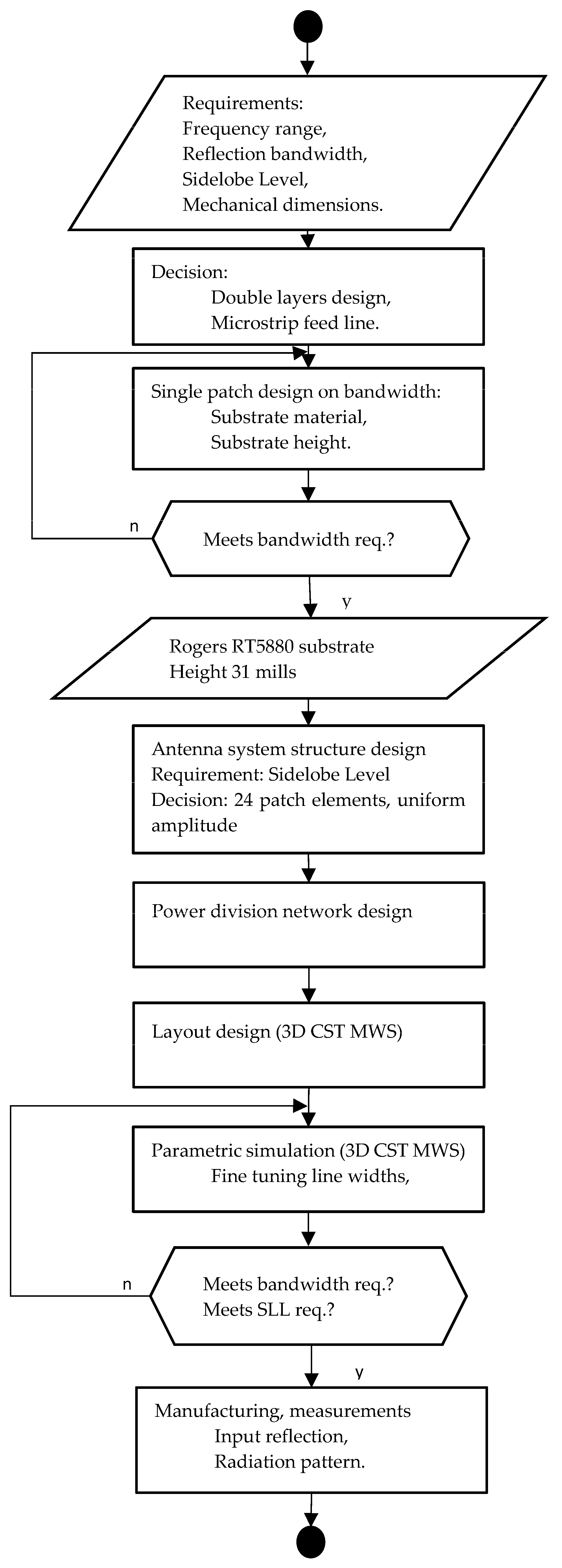
Figure 3.
Flowchart of the antenna overall design procedure.

Figure 4.
Single radiator Microstrip Planar Antenna (Ansys Designer model).

Figure 5.
(a) Single radiator Microstrip Planar Antenna input reflection. (b) Single radiator Microstrip Planar Antenna radiation pattern.
Figure 5.
(a) Single radiator Microstrip Planar Antenna input reflection. (b) Single radiator Microstrip Planar Antenna radiation pattern.

Figure 6.
(a) A 6 × 6 planar uniform rectangular array. (b) 24-element array.

Figure 7.
The E and H plane radiation pattern of rectangular 6 × 6 array.

Figure 8.
The E and H plane radiation pattern of 24 elements array.

Figure 9.
The 24 elements array layout.

Figure 10.
(a) Power division network for a 1 to 4 power ratio, with ideal transmission lines. (b) Power division network for a 1 to 4 power ratio. Microstrip radiators with microstrip transmission line transformers.
Figure 10.
(a) Power division network for a 1 to 4 power ratio, with ideal transmission lines. (b) Power division network for a 1 to 4 power ratio. Microstrip radiators with microstrip transmission line transformers.

Figure 11.
Input reflection of the power division network for a 1 to 4 power ratio, with ideal transmission lines.
Figure 11.
Input reflection of the power division network for a 1 to 4 power ratio, with ideal transmission lines.

Figure 12.
Power ratio for the four radiators of the power division network for 1 to 4 power ratio, with ideal transmission lines.
Figure 12.
Power ratio for the four radiators of the power division network for 1 to 4 power ratio, with ideal transmission lines.

Figure 13.
(a) Power division network from 1 to 4:2:4 power ratio, with ideal transmission lines. (b) Power division network from 1 to 4:2:4 power ratio. Microstrip radiators with microstrip transmission line transformers and the power values are indicated.
Figure 13.
(a) Power division network from 1 to 4:2:4 power ratio, with ideal transmission lines. (b) Power division network from 1 to 4:2:4 power ratio. Microstrip radiators with microstrip transmission line transformers and the power values are indicated.


Figure 14.
Input reflection of the power division network from 1 to 4:2:4 power ratio, with ideal transmission lines.
Figure 14.
Input reflection of the power division network from 1 to 4:2:4 power ratio, with ideal transmission lines.

Figure 15.
Power ratio for the radiators of the power division network for 1 to 4:2:4 power ratio, with ideal transmission lines.
Figure 15.
Power ratio for the radiators of the power division network for 1 to 4:2:4 power ratio, with ideal transmission lines.

Figure 16.
Two-stage quarter wavelength transformers.

Figure 17.
(a) Power division network for 1 to 2:10:10:2 power ratio, with ideal transmission lines. (b) Power division network for 1 to 2:10:10:2 power ratio. Microstrip radiators with microstrip transmission line transformers and the power values are indicated.
Figure 17.
(a) Power division network for 1 to 2:10:10:2 power ratio, with ideal transmission lines. (b) Power division network for 1 to 2:10:10:2 power ratio. Microstrip radiators with microstrip transmission line transformers and the power values are indicated.


Figure 18.
Input reflection of the power division network for 1 to 2:10:10:2 power ratio, with ideal transmission lines.
Figure 18.
Input reflection of the power division network for 1 to 2:10:10:2 power ratio, with ideal transmission lines.

Figure 19.
Power ratio for the radiators of the power division network for 1 to 2:10:10:2 power ratio, with ideal transmission lines.
Figure 19.
Power ratio for the radiators of the power division network for 1 to 2:10:10:2 power ratio, with ideal transmission lines.

Figure 20.
(a) CST MWS model of the microstrip antenna array with 24 elements, without SLL suppression ring. (b) CST MWS model of the microstrip antenna array with 24 elements, with an SLL suppression ring.
Figure 20.
(a) CST MWS model of the microstrip antenna array with 24 elements, without SLL suppression ring. (b) CST MWS model of the microstrip antenna array with 24 elements, with an SLL suppression ring.

Figure 21.
The radiation pattern of the microstrip antenna array with 24 elements, simulated with CST MWS, without, and with an SLL suppression ring (Phi = 0 plane).
Figure 21.
The radiation pattern of the microstrip antenna array with 24 elements, simulated with CST MWS, without, and with an SLL suppression ring (Phi = 0 plane).

Figure 22.
The radiation pattern of the microstrip antenna array with 24 elements, simulated with CST MWS, without, and with an SLL suppression ring (Phi = 90 planes).
Figure 22.
The radiation pattern of the microstrip antenna array with 24 elements, simulated with CST MWS, without, and with an SLL suppression ring (Phi = 90 planes).

Figure 23.
Microstrip antenna array with 24 elements.

Figure 24.
Microstrip antenna connector and radome.

Figure 25.
Microstrip antenna input reflection.

Figure 26.
Microstrip antenna measured radiation pattern.


Table 1.
Comparison of single MPA on different substrates for Bandwidth and Efficiency.
| Substrate | RT5880 εr = 2.2 tan δ = 0.0009 | RO4003 εr = 3.55 tan δ = 0.0027 | RO3010 εr = 10.2 tan δ = 0.0035 | |||
|---|---|---|---|---|---|---|
| Height [mils] | BW [%] | Efficiency [%] | BW [%] | Efficiency [%] | BW [%] | Efficiency [%] |
| 5 | 0.9 | 96.1 | 0.8 | 92.8 | 0.3 | 88.7 |
| 10 | 1.9 | 92.5 | 1.6 | 86.6 | 0.8 | 79.7 |
| 20 | 4.2 | 86.1 | 3.4 | 76.3 | 1.7 | 66.3 |
| 31 | 6.9 | 80.0 | 6.2 | 67.6 | 3.2 | 55.9 |
| 62 | 16.8 | 66.6 | 16.6 | 51.0 | 9.3 | 38.8 |
Table 2.
Comparison of uniform 6 × 6 and 24 elements array.
| Array | Gain [dB] | Beamwidth [deg] | SLL [dB] |
|---|---|---|---|
| 6 × 6 uniform | 22.1 | 14 | −13.7 |
| 24 elements | 20.6 | 17.4 | −15.8 |
Table 3.
Comparison of antenna radiation patterns.
| Gain [dB] | Beamwidth [deg] HH | Beamwidth [deg] VV | SLL [dB] | |
|---|---|---|---|---|
| Simulation | 18.4 | 15 | 21 | −15.7 |
| Measurement | 18.0 | 16 | 19 | −17.3 |
The main parameters of the antenna are Reflection bandwidth = 2.2 GHz (8.8%), Gain = 18 dB, Sidelobe level = −17.3 dB.
Disclaimer/Publisher’s Note: The statements, opinions and data contained in all publications are solely those of the individual author(s) and contributor(s) and not of MDPI and/or the editor(s). MDPI and/or the editor(s) disclaim responsibility for any injury to people or property resulting from any ideas, methods, instructions or products referred to in the content. |
© 2023 by the author. Licensee MDPI, Basel, Switzerland. This article is an open access article distributed under the terms and conditions of the Creative Commons Attribution (CC BY) license (https://creativecommons.org/licenses/by/4.0/).
Share and Cite
MDPI and ACS Style
Nagy, L. Microstrip Antenna Development for Radar Sensor. Sensors 2023, 23, 909. https://doi.org/10.3390/s23020909
AMA Style
Nagy L. Microstrip Antenna Development for Radar Sensor. Sensors. 2023; 23(2):909. https://doi.org/10.3390/s23020909
Chicago/Turabian StyleNagy, Lajos. 2023. "Microstrip Antenna Development for Radar Sensor" Sensors 23, no. 2: 909. https://doi.org/10.3390/s23020909
Note that from the first issue of 2016, this journal uses article numbers instead of page numbers. See further details here.